
Water Cycles and Geothermal Processes in a Volcanic Crater Lake


Abstract
:1. Introduction
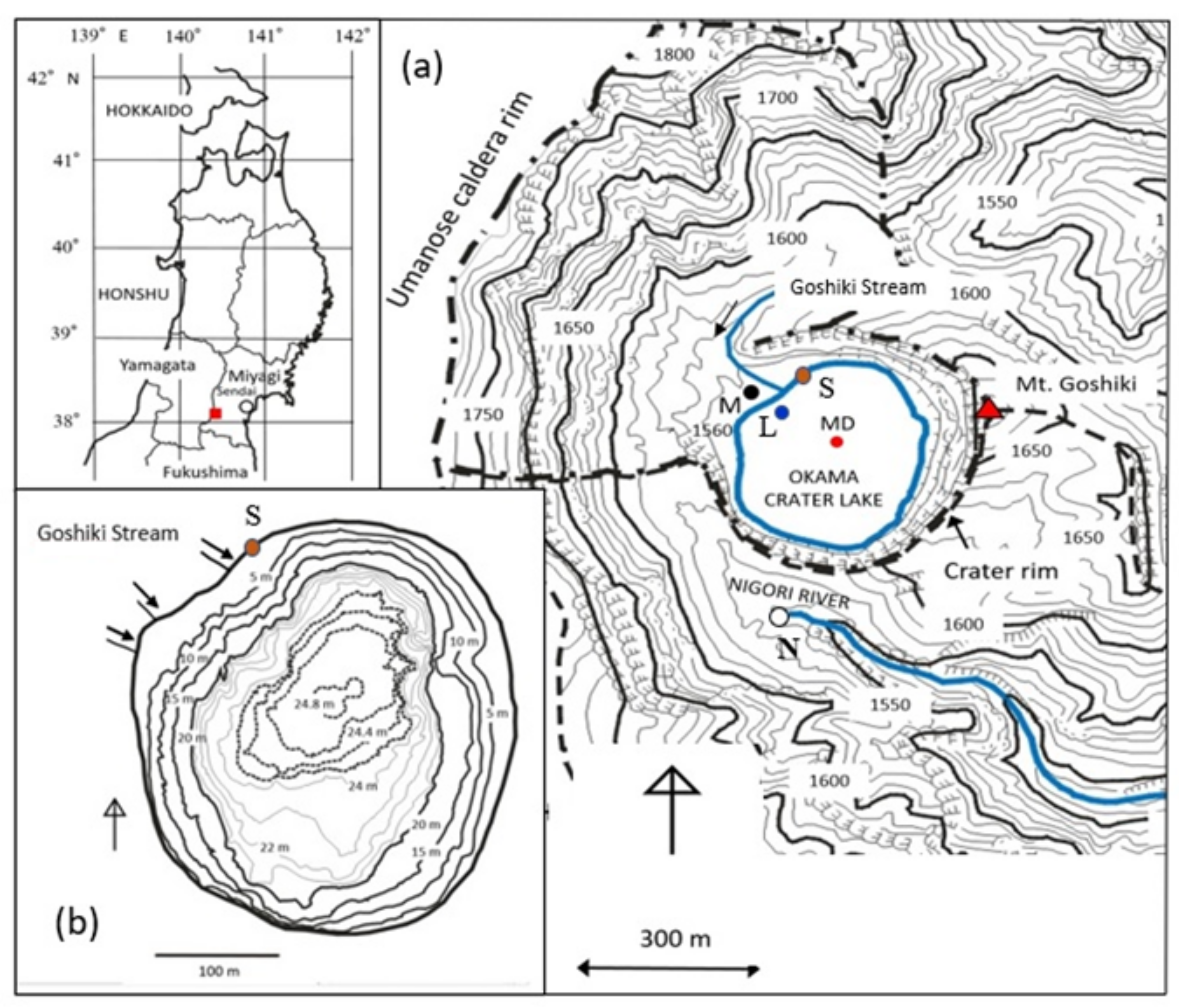
2. Study Area
3. Methods
3.1. Hydrological Budget Estimate for Okama
3.2. Chemical Budget Estimate for Okama
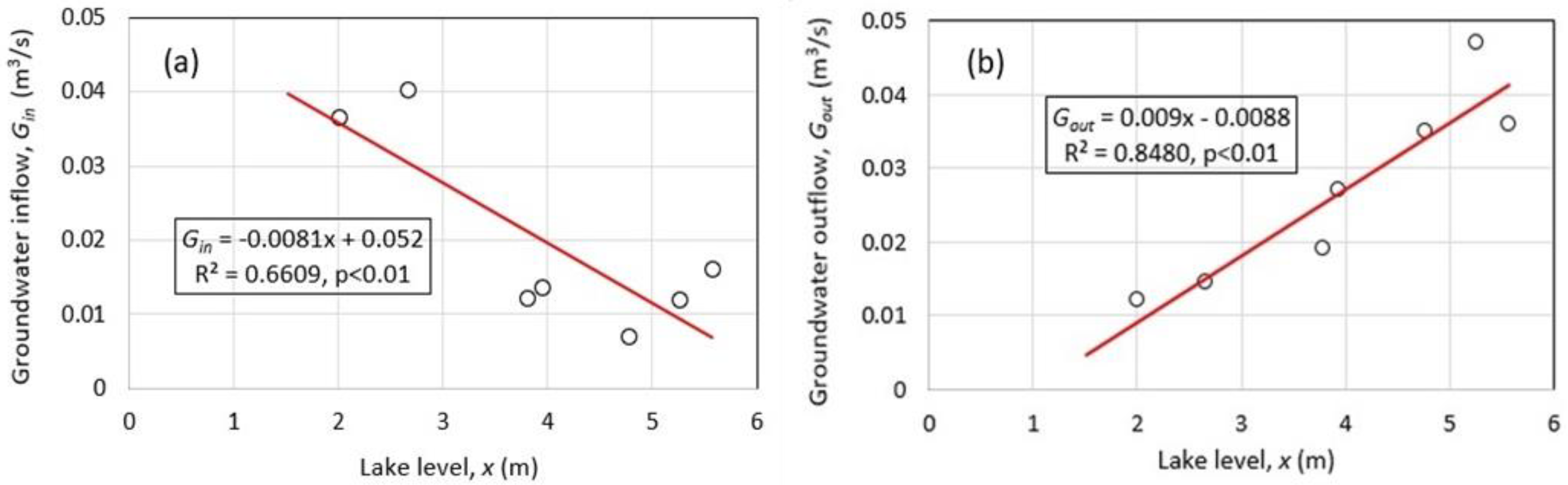
3.3. Evaluation of Groundwater Inflow and Outflow for Okama
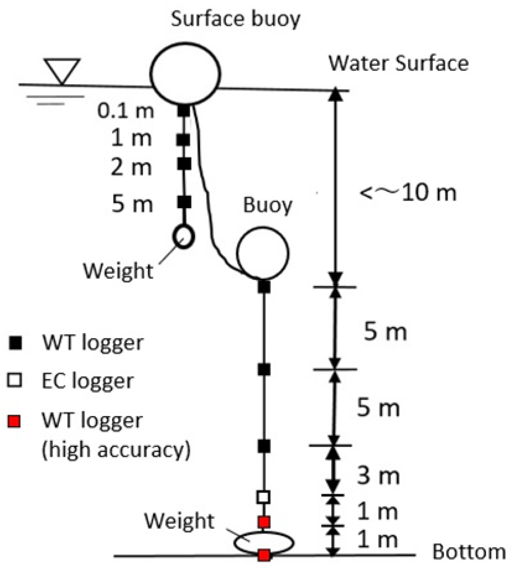
3.4. Field Observations
3.5. Laboratory Experiments
4. Results
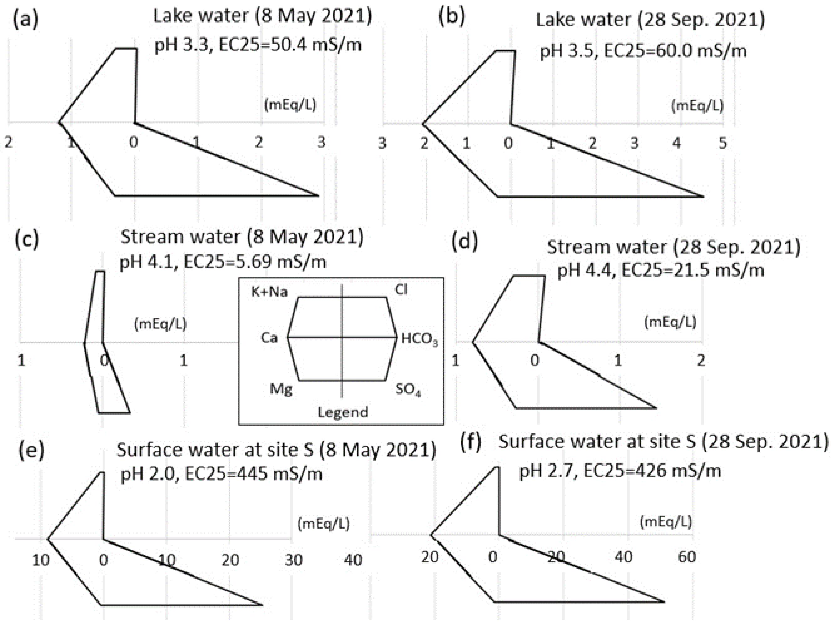
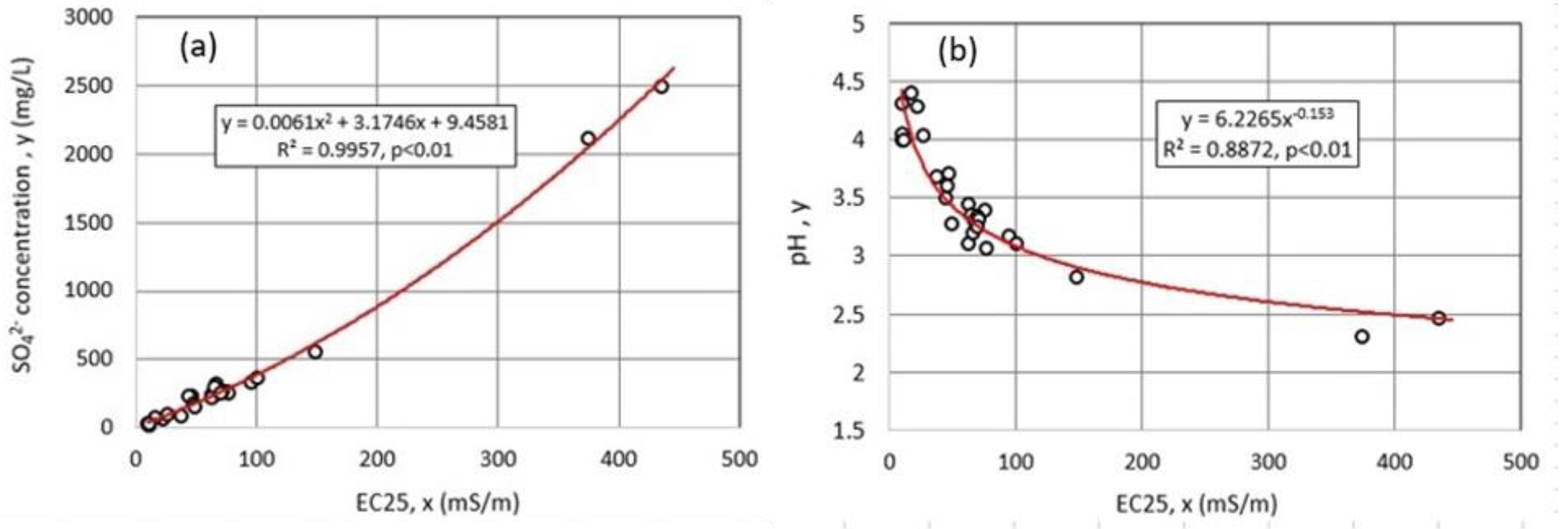
4.1. Water Chemistry
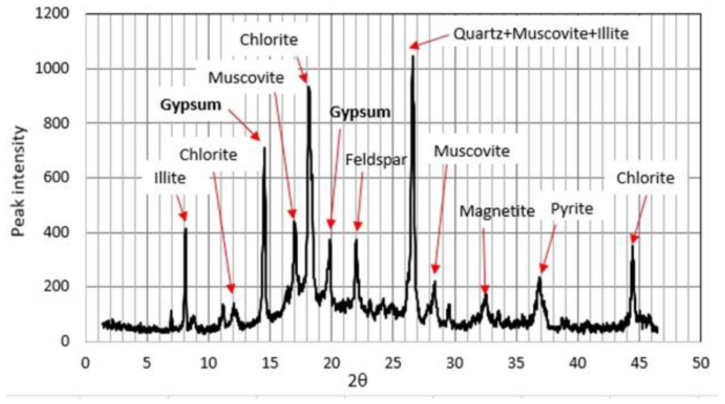
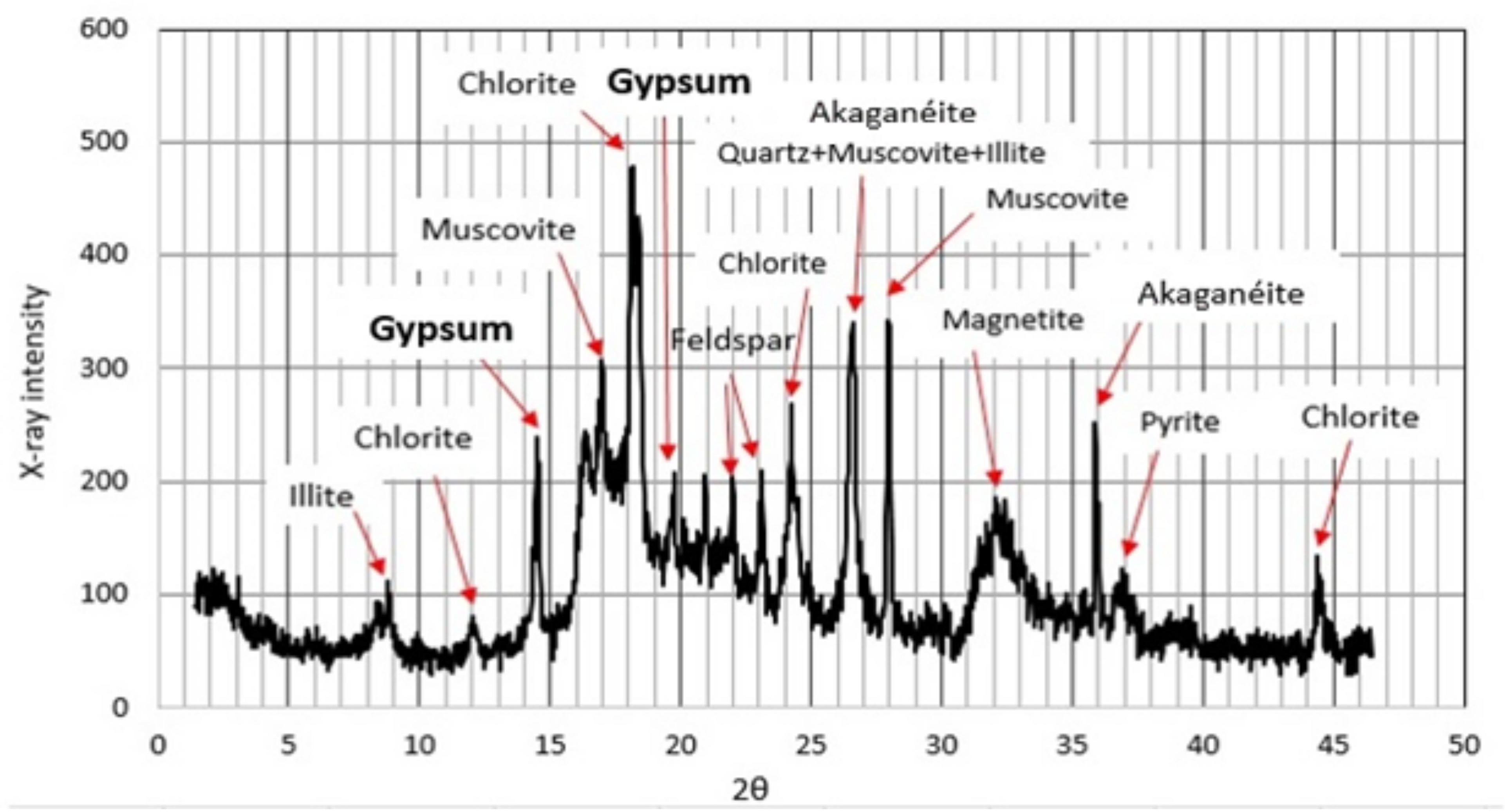
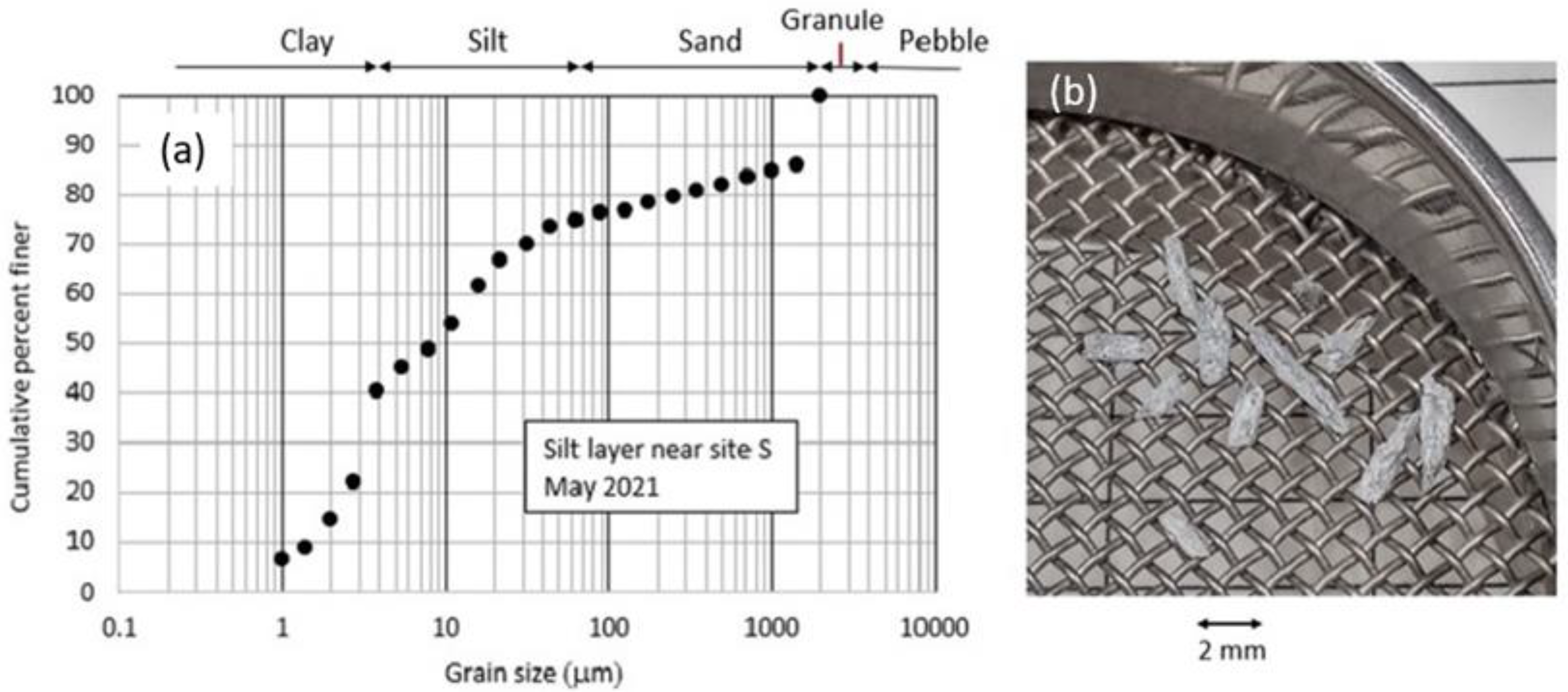
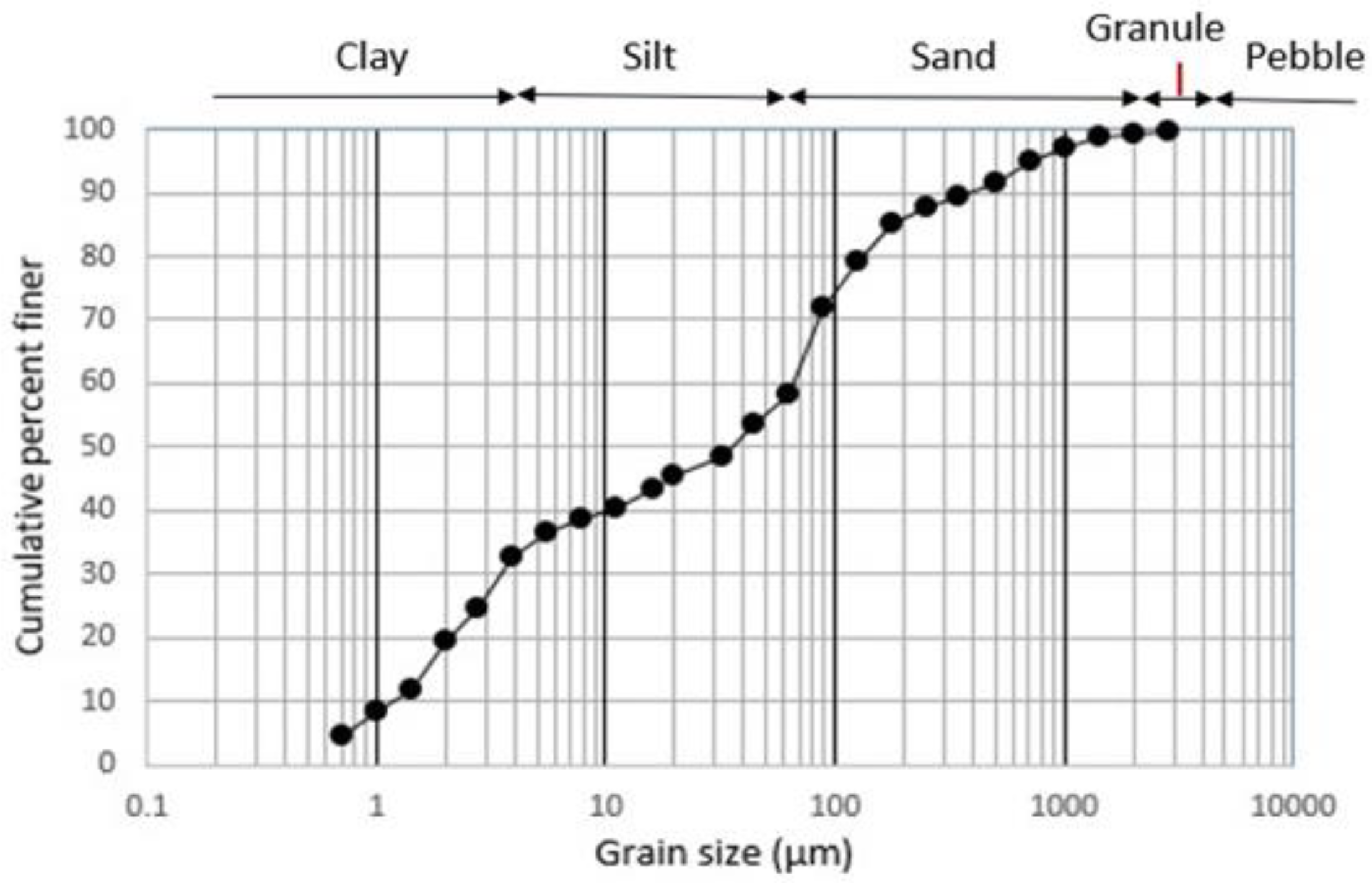
4.2. Mineralogy and Grain Size of the Silty Layer
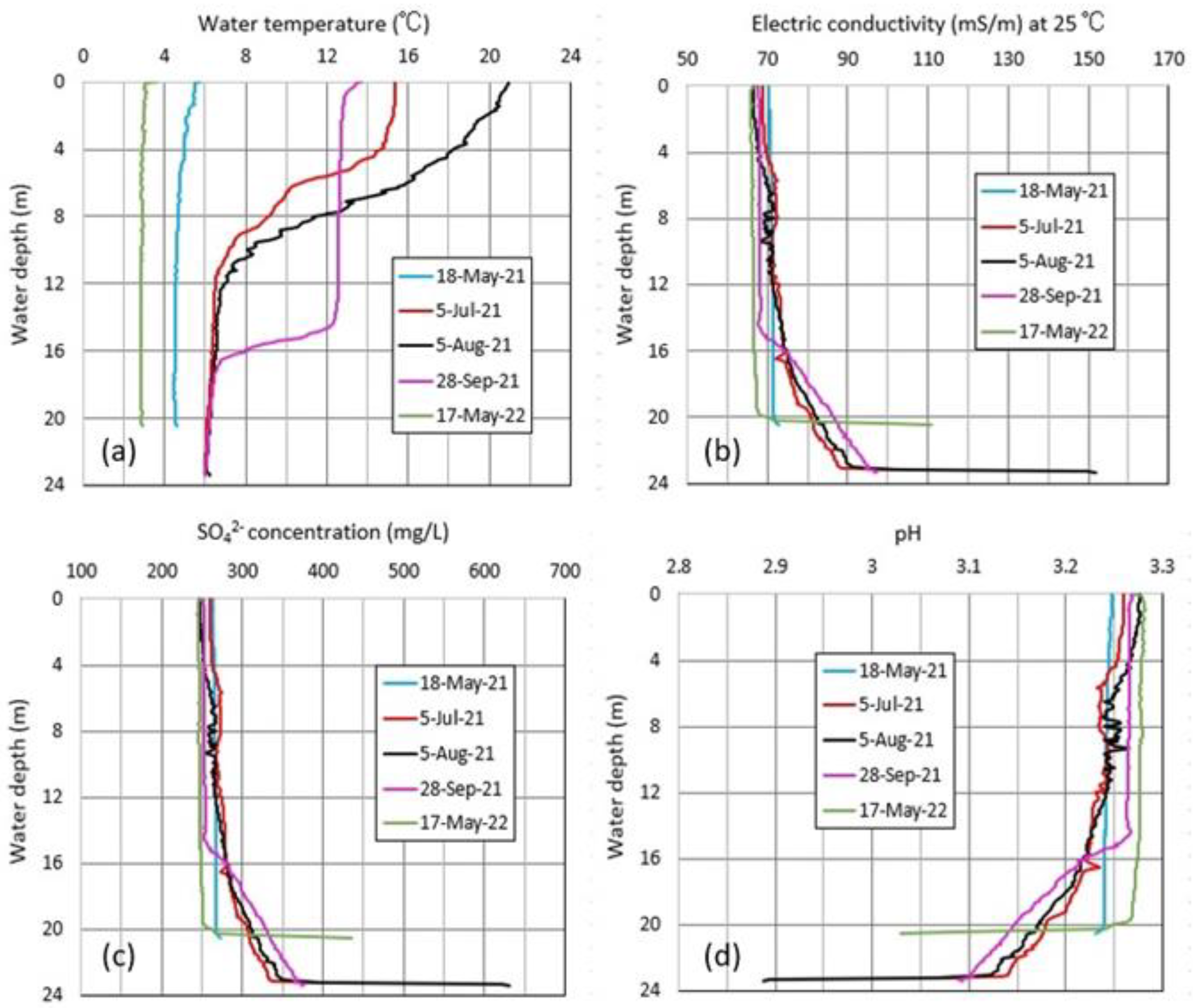
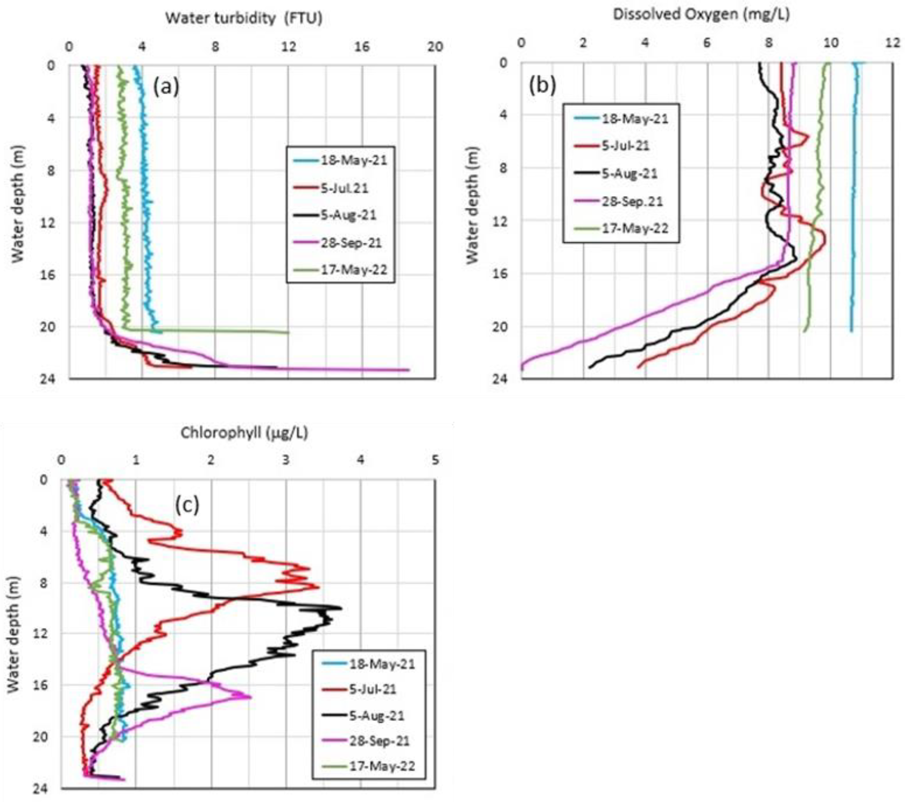
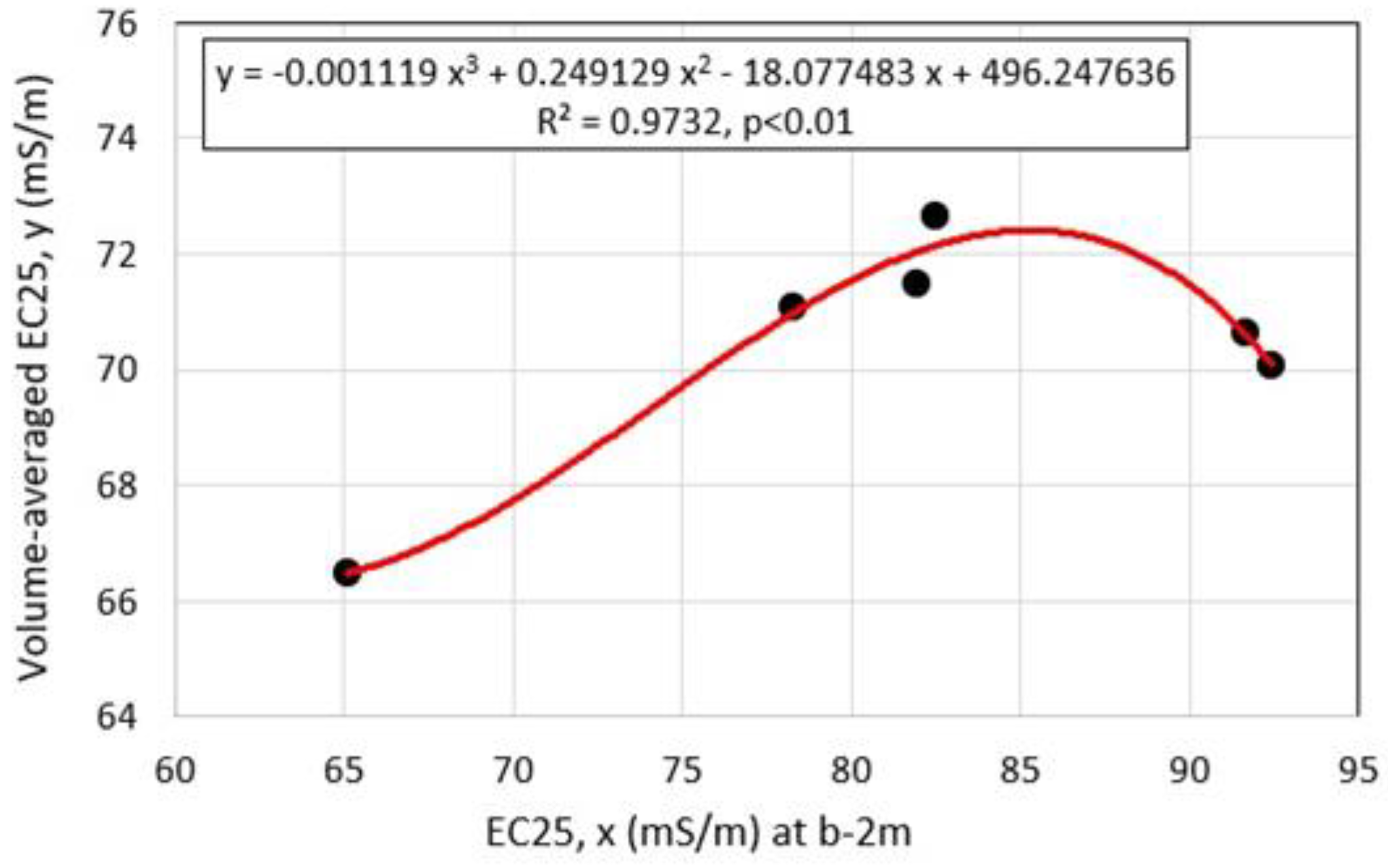
4.3. Vertical Distributions of Water Chemistry in Okama
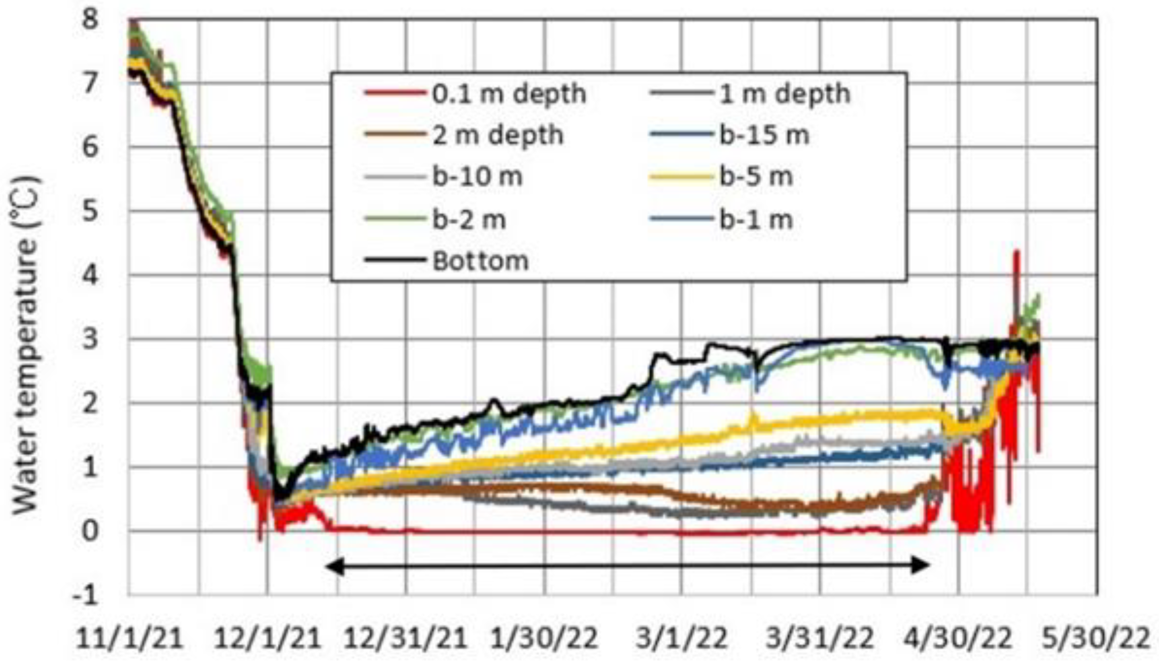
4.4. Thermal Variations in Okama
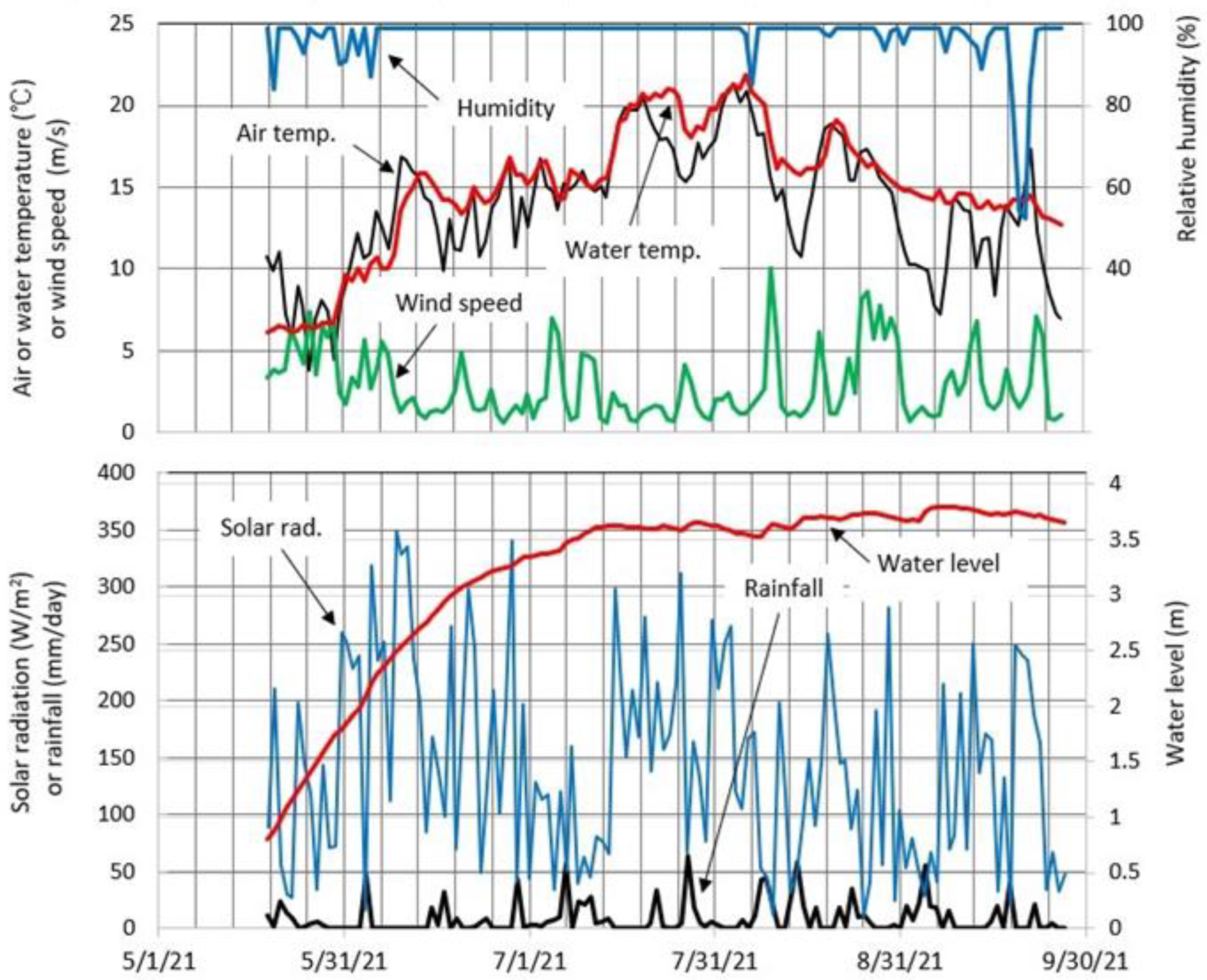
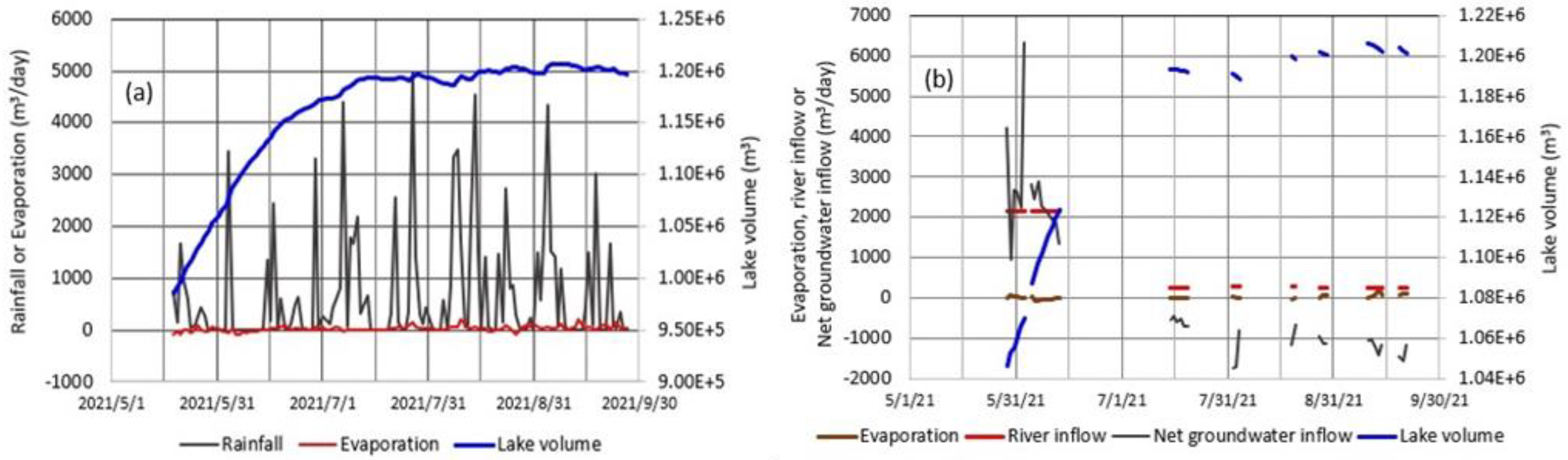
4.5. Meteorology and Lake Level at Okama
5. Discussion
5.1. Geothermal Heat Flux in Okama
5.2. Contribution of Each Hydrological Term to Lake Volume
5.3. Evaluating Groundwater Inflow and Outflow in Okama
6. Conclusions
Author Contributions
Funding
Data Availability Statement
Acknowledgments
Conflicts of Interest
Appendix A

| Symbol | Parameter | Unit |
|---|---|---|
| A0 | Lake surface area | m2 |
| aE | Dimensionless bulk transfer coefficient for latent heat | Non-dimensional |
| E | Evaporation | mm/day, m/s |
| ez | Water vapor pressure at z | Pa |
| e0 | Saturated water vapor pressure at lake surface temperature | Pa |
| Gin | Groundwater inflow | m3/s, m3/day |
| Gout | Groundwater outflow | m3/s, m3/day |
| V | Lake water volume | m3 |
| t | time | sec, day |
| P | Precipitation | mm/h, mm/day, m/day, m/s |
| p | Air pressure | Pa |
| QE | Latent heat flux for evaporation | W/m2 |
| Rin | Stream inflow | m3/s, m3/day |
| uz | Wind speed | m/s |
| z | Height above the lake surface | m |
| β | Ratio of water vapor density to dray air density | Non-dimensional |
| λ | Latent heat for evaporation | J/kg |
| ra | Air density | kg/m3 |
| rw | Water density | kg/m3 |
| CRin | Ionic concentration of inflowing stream water | g/L |
| CP | Ionic concentration of precipitation | g/L |
| CGin | Ionic concentration of inflowing groundwater | g/L |
| CL | Volume-averaged ionic concentration of lake water | g/L |
| S | Net depositional flux | Kg/s |
Appendix B
| Sample | Date | Ionic Concentration (mEq/L) | ||||||
| Na+ | K+ | Ca2+ | Mg2+ | Cl− | HCO3− | SO42− | ||
| Okama water | 8 May 2021 | 0.277 | 0.027 | 1.209 | 0.318 | 0.041 | 0.00 | 2.906 |
| 28 September 2021 | 0.313 | 0.047 | 2.091 | 0.314 | 0.100 | 0.00 | 4.518 | |
| Goshiki water | 8 May 2021 | 0.072 | 0.011 | 0.212 | 0.050 | 0.029 | 0.00 | 0.333 |
| 28 September 2021 | 0.261 | 0.041 | 0.796 | 0.268 | 0.081 | 0.00 | 1.439 | |
| Surface water at site S | 8 May 2021 | 0.471 | 0.034 | 8.938 | 0.467 | 0.029 | 0.00 | 25.32 |
| 28 September 2021 | 1.217 | 0.055 | 21.354 | 1.534 | 0.067 | 0.00 | 51.21 | |
References
- Jasim, A.; Hemmings, B.; Mayer, K.; Bettina Scheu, B. Groundwater flow and volcanic unrest. In Volcanic Unrest; Gottsmann, J., Neuberg, J., Scheu, B., Eds.; Advances in Volcanology; Springer: Cham, Switzerland, 2019; pp. 83–99. [Google Scholar] [CrossRef] [Green Version]
- Niida, K.; Katsui, Y.; Suzuki, T.; Kondō, Y. The 1977–1978 Eruption of Usu Volcano. J. Fac. Sci. Hokkaido Univ. Ser. 4 Geol. Mineral. 1980, 19, 357–394. Available online: https://eprints.lib.hokudai.ac.jp/dspace/handle/2115/36693 (accessed on 20 January 2023).
- Akita, F.; Tsuneda, Y.; Urakami, K. Thermal water flow system in the Toya-ko hot spring area, southwestern Hokkaido, Japan. J. Hot Spring Sci. 2003, 50, 204–220. Available online: http://www.j-hss.org/journal/back_number/vol50_pdf/vol50no4_204_220.pdf (accessed on 20 January 2023).
- Tomiya, A.; Miyagi, I.; Hoshizumi, H.; Yamamoto; Kawanabe, Y.; Satoh, H. Essential material of the March 31, 2000 eruption of Usu Volcano: Implication for the mechanism of the phreatomagmatic eruption. Bull. Geol. Surv. Jpn. 2001, 52, 215–229. Available online: https://www.gsj.jp/data/bulletin/52_04_11.pdf (accessed on 20 January 2023). [CrossRef] [Green Version]
- Goto, A.; Kagiyama, T.; Miyamoto, T.; Yokoo, A.; Taniguchi, H. Long-term prediction of Usu volcano 2000 eruptive activity based on the measurements of heat discharge rate. Geophys. Bul. Hokkaido Univ. 2007, 70, 137–144. [Google Scholar] [CrossRef]
- Chikita, K.A.; Ochiai, Y.; Oyagi, H.; Sakata, Y. Geothermal linkage between a hydrothermal pond and a deep lake: Kuttara Volcano, Japan. Hydrology 2019, 6, 4. [Google Scholar] [CrossRef] [Green Version]
- Chikita, K.A.; Goto, A.; Okada, J.; Yamaguchi, T.; Miura, S.; Yamamoto, M. Hydrological and chemical budgets of Okama Crater Lake in active Zao Volcano, Japan. Hydrology 2022, 9, 28. [Google Scholar] [CrossRef]
- Whiteford, P.C. Evidence for Geothermal Areas Beneath Lake Taupo from Heat Flow Measurements. In Proceedings of the 14th New Zealand Geothermal Workshop, Auckland, New Zealand, 4–6 November 1992; pp. 185–188. Available online: https://www.geothermal-energy.org/pdf/IGAstandard/NZGW/1992/Whiteford.pdf (accessed on 20 January 2023).
- Tivey, M.A.; de Ronde, C.E.J.; Tontini, F.C.; Walker, S.L.; Fornari, D.J. A novel heat flux study of a geothermally active lake—Lake Rotomahana, New Zealand. J. Volcan. Geotherm. Res. 2016, 314, 95–109. [Google Scholar] [CrossRef]
- Candela-Becerra, L.J.; Toyos, G.; Suárez-Herrera, C.A.; Castro-Godoy, S.; Agusto, M. Thermal evolution of the Crater Lake of Copahue Volcano with ASTER during the last quiescence period between 2000 and 2012 eruptions. J. Volcan. Geotherm. Res. 2020, 392, 106752. [Google Scholar] [CrossRef]
- Brehme, M.; Giese, R.; Suherlina, L.; Kamah, Y. Geothermal sweetspots identified in a volcanic lake integrating bathymetry and fluid chemistry. Sci. Rep. 2019, 9, 16153. [Google Scholar] [CrossRef] [Green Version]
- Ban, M.; Oikawa, T.; Yamazaki, S. Geologic map of Zao Volcano; Geological Survey of Japan, AIST: Tokyo, Japan, 2015; 8p. [Google Scholar]
- Ban, M.; Oikawa, T.; Yamazaki, S.; Goto, A.; Yamamoto, M.; Miura, S. Prediction of eruption courses in volcanoes without eruptions under modern observation system: Example of Zao Volcano. Volcano 2019, 64, 131–138. [Google Scholar]
- Sendai Reginal Headquarters, JMA. Explanatory Material of Zao Volcano. Explan. Mater. 2023, 1–4. Available online: https://www.data.jma.go.jp/svd/vois/data/tokyo/STOCK/monthly_v-act_doc/sendai/22m12/212_22m12.pdf (accessed on 13 January 2023).
- Konno, Y. Nigori-gawa, an acid stream originated from the crater-lake “Okama” of Mt. Zao. Jpn. J. Limnol. 1936, 6, 21–26. [Google Scholar] [CrossRef]
- Kondo, J. Meteorology in Aquatic Environments; Asakura Publishing Ltd.: Tokyo, Japan, 1994; 350p. [Google Scholar]
- Chikita, K. A field study on turbidity currents initiated from spring runoffs. Water Res. Res. 1989, 25, 257–271. [Google Scholar] [CrossRef]
- Chikita, K.A.; Smith, N.D.; Yonemitsu, N.; Perez-Arlucea, M. Dynamics of sediment-laden underflows passing over a subaqueous sill: Glacier-fed Peyto Lake, Alberta, Canada. Sedimentology 1996, 43, 865–875. [Google Scholar] [CrossRef]
- Asif Ali, A.; Chiang, Y.W.; Santos, R.M. X-ray Diffraction Techniques for Mineral Characterization: A Review for Engineers of the Fundamentals, Applications, and Research Directions. Minerals 2022, 12, 205. [Google Scholar]
- Freedman, L.C.; Erdmann, D.E. Quality assurance practices for the chemical and biological analyses for water and fluvial sediments. In Techniques of Water-Resources Investigations of the United States Geological Survey; US Government Printing Office: Washington, DC, USA, 1982; Chapter A6; 181p. [Google Scholar]
- Yanagisawa, F.; Nakagawa, N.; Abe, H.; Yano, K. Chemical composition of snow cover and rime at Mt. Zao, Yamagata Prefecture, Japan. Seppyo 1995, 58, 393–403. [Google Scholar] [CrossRef] [Green Version]
- van Hinsberg, V.J.; Berlo, K.; Pinti, D.L.; Ghaleb, B. Gypsum precipitation from volcanic effluent as an archive of volcanic activity. Front. Earth Sci. 2021, 9, 764087. [Google Scholar] [CrossRef]
- Bunaciu, A.A.; UdriŞTioiu, G.E.; Aboul-Enein, H.Y. X-ray diffraction: Instrumentation and applications. Crit. Rev. Anal. Chem. 2015, 45, 289–299. [Google Scholar] [CrossRef]
- Horai, H.; Kamei, T.; Ogawa, Y.; Shibi, T. Development of bassanite production system and its geotechnical engineering significance—Recycling of waste plasterboard. Jpn. Geotech. J. 2008, 3, 133–142. [Google Scholar] [CrossRef] [Green Version]
- Adachi, M.; Tanimoto, A. On the equations representing solubility of calcium sulfate in pure water. Gypsum Lime 1975, 135, 17–26. [Google Scholar]
- Singh, N.B.; Middendorf, B. Calcium sulphate hemihydrate hydration leading to gypsum crystallization. Prog. Cryst. Growth Charact. Mater. 2007, 53, 57–77. [Google Scholar] [CrossRef]
- Blodau, C. A review of acidity generation and consumption in acidic coal mine lakes and their watersheds. Sci. Total Environ. 2006, 369, 307–332. [Google Scholar] [CrossRef] [PubMed]
- Kanie, K.; Muramatsu, A.; Suzuki, S.; Waseda, Y. Effects of sulfate irons on conversion of Fe(OH)3 gel to β-FeOOH and α-Fe2O3. Bull. Inst. Adv. Mater. Process. Tohoku Univ. 2005, 60, 21–27. Available online: http://hdl.handle.net/10097/30818 (accessed on 12 February 2023).
- Chikita, K.A. Sedimentation by river-induced turbidity currents: Field measurements and interpretation. Sedimentology 1990, 37, 891–905. [Google Scholar] [CrossRef]
- Lambert, A.M.; Kelts, K.R.; Marshall, N.F. Measurements of density underflows from Walensee, Switzerland. Sedimentology 1976, 23, 87–105. [Google Scholar] [CrossRef]
- Ichiki, M.; Kaida, T.; Yamamoto, M.; Miura, S.; Kanda, W.; Ushioda, M.; Seki, K.; Morita, Y.; Uyeshima, M. An electrical resistivity exploration of Zao volcano, using audio-frequency magnetotelluric method to evaluate the eruption potential field. In Proceedings of the Fall Meeting 2021, Online, 20–22 October 2021; Volcanological Society of Japan: Hokkaido, Japan, 2021; pp. 1–14. [Google Scholar]
- Umetsu, Y. Gypsum from neutralization of sulfuric acid solution with lime stone. Gypsum Lime 1991, 234, 31–37. [Google Scholar] [CrossRef]
- Ozair, G. An overview of calcium carbonate saturation indices as a criterion to protect desalinated water transmission lines from deterioration. Nat. Environ. Pollut. Technol. 2012, 11, 203–212. Available online: https://neptjournal.com/index.php/search/Ozair (accessed on 13 February 2023).


| No. | Period | Lake Level (m) | Gin − Gout (m3/s) | Gin (m3/s) | Gout (m3/s) |
|---|---|---|---|---|---|
| (1) | 3–6 August 2020 | 5.57 | −0.020 | 0.016 | 0.036 |
| (2) | 19–28 August 2020 | 5.26 | −0.035 | 0.012 | 0.047 |
| (3) | 30 September–4 October 2020 | 4.78 | −0.028 | 0.007 | 0.035 |
| (4) | 29 May–3 June 2021 | 1.83 | 0.025 | 0.037 | 0.012 |
| (5) | 5–13 June 2021 | 2.48 | 0.026 | 0.040 | 0.014 |
| (6) | 15–20 July 2021 | 3.62 | −0.007 | 0.012 | 0.019 |
| (7) | 10–14 September 2021 | 3.77 | −0.013 | 0.014 | 0.027 |
Disclaimer/Publisher’s Note: The statements, opinions and data contained in all publications are solely those of the individual author(s) and contributor(s) and not of MDPI and/or the editor(s). MDPI and/or the editor(s) disclaim responsibility for any injury to people or property resulting from any ideas, methods, instructions or products referred to in the content. |
© 2023 by the authors. Licensee MDPI, Basel, Switzerland. This article is an open access article distributed under the terms and conditions of the Creative Commons Attribution (CC BY) license (https://creativecommons.org/licenses/by/4.0/).
Share and Cite
Chikita, K.A.; Goto, A.; Okada, J.; Yamaguchi, T.; Oyagi, H. Water Cycles and Geothermal Processes in a Volcanic Crater Lake. Hydrology 2023, 10, 54. https://doi.org/10.3390/hydrology10030054
Chikita KA, Goto A, Okada J, Yamaguchi T, Oyagi H. Water Cycles and Geothermal Processes in a Volcanic Crater Lake. Hydrology. 2023; 10(3):54. https://doi.org/10.3390/hydrology10030054
Chicago/Turabian StyleChikita, Kazuhisa A., Akio Goto, Jun Okada, Takashi Yamaguchi, and Hideo Oyagi. 2023. "Water Cycles and Geothermal Processes in a Volcanic Crater Lake" Hydrology 10, no. 3: 54. https://doi.org/10.3390/hydrology10030054