Assessing the Potential of Combined SMAP and In-Situ Soil Moisture for Improving Streamflow Forecast

Abstract

Soil moisture is an essential hydrological variable for a suite of hydrological applications. Its spatio-temporal variability can be estimated using satellite remote sensing (e.g., SMOS and SMAP) and in-situ measurements. However, both have their own strengths and limitations. For example, remote sensing has the strength of maintaining the spatial variability of near-surface soil moisture, while in-situ measurements are accurate and preserve the dynamics range of soil moisture at both surface and larger depths. Hence, this study is aimed at (1) merging the strength of SMAP with in-situ measurements and (2) exploring the effectiveness of merged SMAP/in-situ soil moisture in improving ensemble streamflow forecasts. The conditional merging technique was adopted to merge the SMAP-enhanced soil moisture (9 km) and its downscaled version (1 km) separately with the in-situ soil moisture collected over the au Saumon watershed, a 1025 km² watershed located in Eastern Canada. The random forest machine learning technique was used for downscaling of the near-surface SMAP-enhanced soil moisture to 1 km resolution, whereas the exponential filter was used for vertical extrapolation of the SMAP near-surface soil moisture. A simple data assimilation technique known as direct insertion was used to update the topsoil layer of a physically-based distributed hydrological model with four soil moisture products: (1) the merged SMAP/in-situ soil moisture at 9 and 1 km resolutions; (2) the original SMAP-enhanced (9 km), (3) downscaled SMAP-enhanced (1 km), and (4) interpolated in-situ surface soil moisture. In addition, the vertically extrapolated merged SMAP/in-situ soil moisture and subsurface (rootzone) in-situ soil moisture were used to update the intermediate layer of the model. Results indicate that downscaling of the SMAP-enhanced soil moisture to 1 km resolution improved the spatial variability of soil moisture while maintaining the spatial pattern of its original counterpart. Similarly, merging of the SMAP with in- situ soil moisture preserved the dynamic range of in-situ soil moisture and maintained the spatial heterogeneity of SMAP soil moisture. Updating of the top layer of the model with the 1 km merged SMAP/in-situ soil moisture improved the ensemble streamflow forecast compared to the model updated with either the SMAP-enhanced or in-situ soil moisture alone. On the other hand, updating the top and intermediate layers of the model with surface and vertically extrapolated SMAP/in-situ soil moisture, respectively, did not further improve the accuracy of the ensemble streamflow forecast. Overall, this study demonstrated the potential of merging the SMAP and in-situ soil moisture for streamflow forecast.

1. Introduction

Soil moisture plays a paramount role in the land–atmosphere interactions by controlling the exchange of water and energy between the land surface and the atmosphere [1,2] and this in turn controls a number of hydrological processes including infiltration, evapotranspiration and runoff generation. It also plays an essential role in many hydrometeorological and agricultural applications including flood forecasting, weather forecasting and irrigation water management [3].

Knowledge of soil moisture spatial and temporal variability is important to improve our understanding of its role in hydrological processess and applications. Traditionally, in-situ measurements are used to characterize the spatio-temporal variability of soil moisture, but they are scarce and costly to implement over a large area [4]. On the other hand, remote sensing has become an invaluable alternative for global mapping of near-surface soil moisture in recent decades [5,6].

Passive microwave remote sensing at lower frequency bands (e.g., L-band) has become an established technique for mapping of near-surface soil moisture (i.e., up to 5–10 cm) because of its high sensitivity to soil moisture and high capability to penetrate through cloud and vegetation canopy, notably at low to moderate vegetation density [7,8]. Currently, there are two L-band passive microwave satellite missions which are fully dedicated to soil moisture measurements: Soil Moisture and Ocean Salinity (SMOS) and Soil Moisture Active Passive (SMAP). Besides the L-band, there are other sensors with X- and C-bands such as the Advanced Microwave Scanning Radiometer (AMSR-E/2), the Special Sensor microwave/Imager (SSM/I) and the Special Sensor Microwave Imager/Sounder (SSMIS) passive microwave sensor have been used to infer soil moisture.

Nevertheless, the coarseness of the resolution of soil moisture products derived from passive microwave satellites remains one of the major challenges for its use at local and regional scale hydrological applications. To address this, many studies have attempted to downscale such soil moisture products, e.g., Abbaszadeh et al. [9], Djamai et al. [10], and Wakigari and Leconte [11]. These studies used a range of downscaling approaches, from simple polynomial fitting based on the universal triangle/trapezoid techniques (e.g., Piles et al. [12], Djamai et al. [10]), to more advanced machine learning techniques such as random forest (e.g., Bai et al. [13], Wakigari and Leconte [11]), neural network (e.g., Alemohammad et al. [14]) and support vector machines (e.g., Srivastava et al. [15]).

Given the increasing availability of remotely sensed soil moisture products, their assimilation into hydrological models for improving streamflow simulation and forecast has received much attention in recent decades. A number of studies have assimilated soil moisture derived from different satellites (e.g., SMOS, SMAP, AMSR-E and Sentinel-1) into different hydrological models to improve the accuracy streamflow simulation and forecast [16,17,18,19]. However, the degree of improvement varies from no [20] or minor improvement [21] to marked improvement [22,23]. Indeed, it is difficult to compare and generalize the results of these studies as they are based on different soil moisture assimilation techniques (e.g., ensemble Kalman filter, direct insertion or particle filter), model structures (fully/semi-distributed and lumped) and physiographic characteristics of the watershed among many others [24,25].

When looking specifically at the effect of physiographic characteristics among the stated factors, the success of assimilation of remotely sensed soil moisture critically depends on the quality of the assimilated soil moisture product [26], which in turn depends on the study area’s physiographic characteristics. For example, in low to moderately vegetated areas, the effect of vegetation on soil moisture retrieval is minimal [5], and this allowed a number of soil moisture assimilation studies to be carried out in such areas to take advantage of good quality soil moisture retrieval [16,19,27].

On the other hand, over densely vegetated areas, it is difficult to obtain satellite soil moisture with the desired accuracy, e.g., the unbiased root-mean-square error (ubRMSE) of 0.04 m³/m³ set by some of the satellite missions such as SMAP and SMOS [5,6]. Hence, we deem that the use of remotely sensed soil moisture products together with in-situ soil moisture measurements would be a potential way forward for such areas. Put differently, the merging of the strengths of SMAP and in-situ soil moisture has the potential to generate a better-quality soil moisture product than any single one of them.

Therefore, the present study aims to explore the utility of the combination of in-situ soil moisture with the SMAP-enhanced soil moisture in improving streamflow forecast skills for a small heavily-forested watershed located in Eastern Canada.

2. Materials and Methods

2.1. Study Area

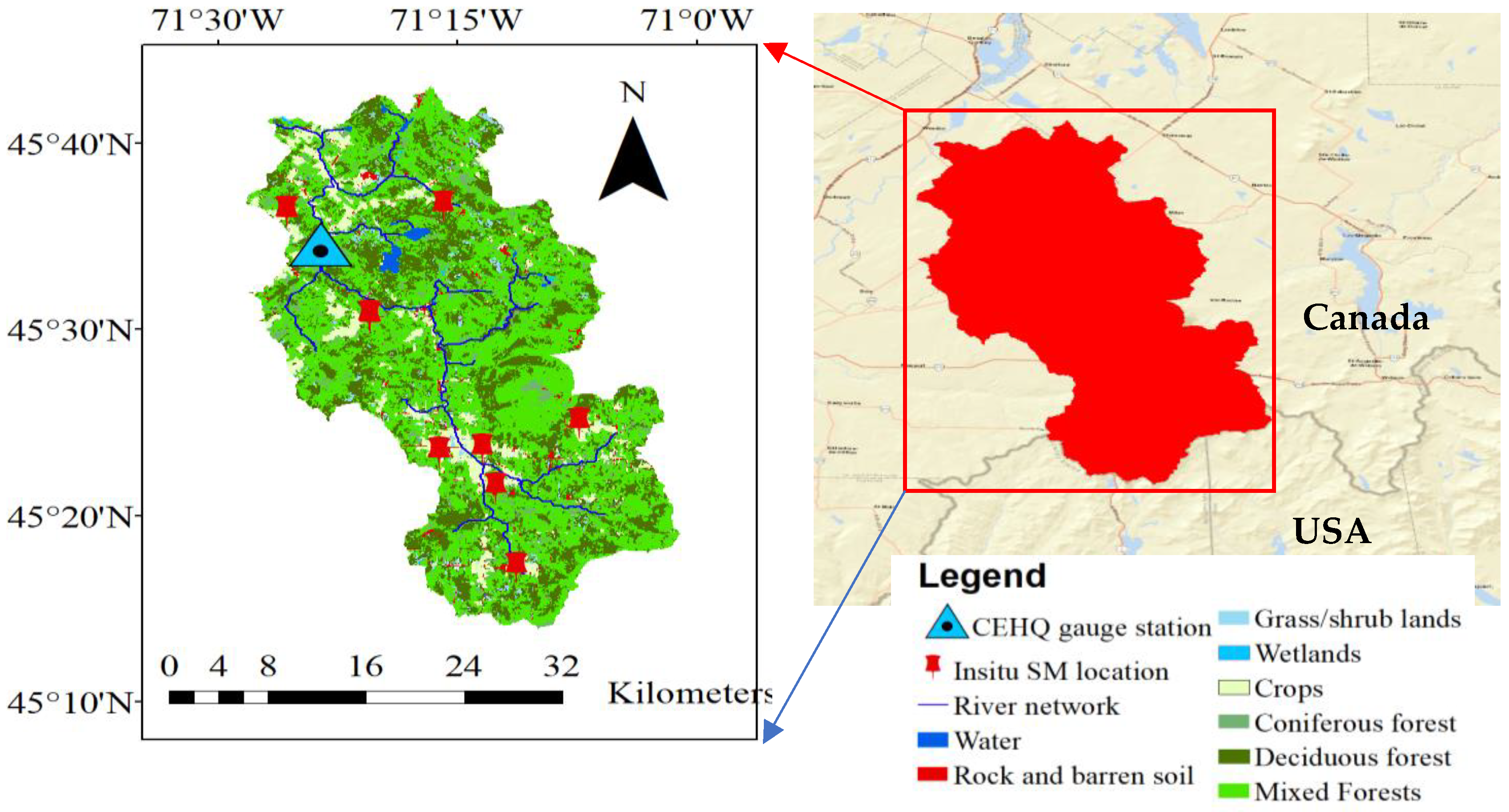
The au Saumon Watershed situated in Eastern Canada was selected for this study (Figure 1). It has a drainage area of 1025 km². It receives annual precipitation (rain and snow) of roughly up to 1250 mm with an average annual temperature of 4.5 °C, whereas the average summer precipitation and temperature are 760 mm and 19.5 °C, respectively. The watershed often experiences high flows in spring and fall from snow melt and rainfall, respectively. Forest is the main land cover type of this watershed. Its elevation varies between 277 and 1092 m.

2.2. Data

2.2.1. SMAP Enhanced Soil Moisture Product

The SMAP-enhanced level 3 passive microwave soil moisture product (SPL3SMP_E) with a daily global coverage was selected for this study. This product is derived from a daily composite of SMAP-enhanced L2 half-orbit products, which in turn is generated from the SMAP-Enhanced L1 Gridded Brightness Temperature Product (L1CTB_E) using the Backus–Gilbert (BG) optimal interpolation technique [28]. SPL3SMP_E has a spatial resolution of 9 km displayed on Equal-Area Scalable Earth (EASE) Grid 2.0. Its descending (06:00 local time) and ascending (18:00 local time) orbits soil moisture products are retrieved separately, yet for the present study the SPL3SMP_E descending product was selected because at this time there is a better thermal equilibrium between soil surface and vegetation layer. These data can be accessed freely from the NASA Snow and Ice Data Center (NSIDC) (https://nsidc.org/data/smap/, accessed on 20 July 2020).

In addition, a downscaled SMAP-enhanced soil moisture to 1 km was used. For downscaling, the random forest (RF) machine learning technique was employed. Its implementation involves training of RF with predictors derived from MODIS such as land surface temperature, NDVI and albedo [11]. In addition, topographic derivatives, such as elevation, slope and aspect, were used. Training was carried out at resolution of the SMAP-enhanced product which is 9 km. After training and testing RF at 9 km spatial resolution, it was used to estimate soil moisture at 1 km from the 1 km resolution predictors, assuming that the developed model is spatial-scale invariant.

2.2.2. In-Situ Soil Moisture

In-situ soil moisture observations collected during the summer season of 2019 over the au Saumon watershed using EC-5 soil moisture probes [29] were used. A total of 8 soil moisture probes were installed at 8 selected representative locations (i.e., open and forested sites) to collect hourly volumetric soil moisture at depths of 5 and 20 cm (sites numbered 1 to 8, see Figure 1).

2.2.3. Hydrometeorological Data

Daily deterministic precipitation and temperature (i.e., maximum and minimum temperature) were derived from MSWEP (Multi-Source Weighted-Ensemble Precipitation) [30] and ERA-5 land [30], respectively, for the period 1980 to 2018 (i.e., for calibration and validation of the model). In addition, the data for the year 2019 were separately extracted for deterministic forecast. Similarly, the daily streamflow observations at station 030282 (draining an area of 769 km²) were obtained from the Centre d’expertise hydrique du Québec (now the Direction de l’expertise hydrique du Québec, a provincial agency whose mandate is to manage Québec’s water regime) for the period 1980 to 2019.

Apart from the deterministic data, an ensemble of daily precipitation and maximum and minimum temperature was forced to the model to produce ensemble streamflow forecasts for the summer season of 2019. The forcing data were extracted from the EM-Earth (the Ensemble Meteorological Dataset for Planet Earth) data [31]. These data have a spatial resolution of roughly 10 km, and they are available from 1950 to 2019. They have 25 ensemble members which can be used for ensemble hydrological simulations.

2.3. Hydrological Model

The HYDROTEL model was selected for experimenting on the effect of assimilation of soil moisture measurements on the accuracy of model prediction. HYDROTEL is a physically based, semi-distributed and continuous time hydrological model developed at the Institut National de la Recherche Scientifique Eau Terre Environnement (INRS-ETE), Québec (Canada) [32]. It has attractive features, such as ease of incorporation of spatially distributed GIS and remotely sensed data such as soil moisture and snow water equivalent and minimal meteorological data requirement (i.e., only precipitation and maximum and minimum temperature).

PHYSITEL, a GIS tool accompanied with HYDROTEL, was used to spatially discretize the watershed into relatively homogeneous hydrological response units (RHHUs) based on elevation, land cover, soil type and river networks. Accordingly, the au Saumon watershed was discretized to 205 RHHUs with an average area of 5.0 km².

HYDROTEL is composed of six modules: (1) interpolation of precipitation, (2) accumulation and melt of snowpack, (3) potential evapotranspiration estimation, (4) vertical water budget (i.e., soil moisture module), (5) surface and subsurface flow generation and (6) river flow routing. Among these modules, the vertical water budget module (i.e., soil module) was used for the incorporation of remotely sensed and in-situ soil moisture observations into the model. This module has two sub-modules: BV3C and CEQUEAU. The BV3C was selected for this study. BV3C vertically discretizes a soil column into three layers. The first layer has a depth which is normally 5 to 10 cm, and it controls the partitioning of rainfall into surface runoff and infiltration. The second and third layers have typical depth of 60 to 80 cm and 120 to 200 cm, respectively, and they are used to control the generation of interflow and baseflow, respectively. The water exchange between the layers is controlled by the Richards-1D equation [33].

The HYDROTEL simulated streamflow was calibrated and validated against the observed daily streamflow at station 030282 (see Figure 1) for the period 1980 to 2008 and 2009 to 2018, respectively. The dynamically dimensioned search-uncertainty analysis (DDS-UA) algorithm [34] was applied for calibration using the Nash–Sutcliffe efficiency (NSE) as the objective function [35]. The Kling–Gupta efficiency (KGE) [36] was also used for evaluation of the model performance. The NSE (Equation (1)) and KGE (Equation (2)) values range between −∞ and 1. An NSE or KGE value of 1 indicates a perfect model performance. In general, the higher the NSE and KGE values, the better the performance of the model and vice versa.

$$NSE=1-\frac{{\sum }_{i=1}^n{\left(Q_{sim,i}-Q_{obs,i}\right)}^2}{{\sum }_{i=1}^n{\left(Q_{obs,i}-{\overline{Q}}_{obs,i}\right)}^2}$$

(1)

$$KGE=\sqrt{{\left(r-1\right)}^2+{\left(\frac{{\sigma }_{sim}}{{\sigma }_{obs}}-1\right)}^2+{\left(\frac{{\mu }_{sim}}{{\mu }_{obs}}-1\right)}^2}$$

(2)

where NSE and KGE are Nash–Sutcliffe efficiency and Kling–Gupta efficiency, respectively, Q_obs and Q_sim are the observed and simulated discharge, respectively, σ_obs and σ_sim are observation and simulated standard deviation, respectively, and µ_obs and µ_sim, are observation and simulation mean_, respectively.

2.4. Merging of SMAP and In-Situ Soil Moisture

The conditional merging technique [37] which was originally developed for merging of radar and rain gauge data was used to merge gridded SMAP soil moisture with that of in-situ soil moisture measurements. This technique was separately applied for merging of (1) the SMAP surface and in-situ surface soil moisture and (2) the vertically extrapolated SMAP and deep layer (20 cm) in-situ soil moisture measurements.

The major advantage of this technique is that it preserves the spatial covariance structure of the grid-based measurement (i.e., SMAP soil moisture) while maintaining the accuracy of in-situ measurements. Its implementation involves six successive steps: (a) extraction of the SMAP grid points that cover the study area, (b) interpolation of in-situ soil moisture measurements (i.e., eight sites shown in Figure 1) using ordinary kriging to the regular grid points of SMAP extracted over the study area as indicated in step a, (c) extraction of the SMAP soil moisture at in-situ soil moisture measurement locations, (d) interpolation of extracted SMAP soil moisture to the regular grid points of SMAP as indicated in step a, (e) estimation of the residual between interpolated SMAP (d) and extracted SMAP soil moisture (a), and (f) addition of the estimated residual to interpolated in-situ soil moisture (b) to produce the final merged SMAP/in-situ soil moisture.

It is worth noting that the SMAP soil moisture is only available every 2 to 3 days over the study area. In contrast, our in-situ soil moisture measurement has daily temporal resolution. Therefore, the conditional merging technique was applied to temporally collocated SMAP and in-situ soil moisture measurements. In other words, only dates when the SMAP and in-situ soil moisture measurements overlap are considered for merging. Indeed, the residual was also estimated for dates when the SMAP and in-situ soil moisture overlap and then added to spatially interpolated in-situ soil moisture for generation of merged SMAP/in-situ soil moisture.

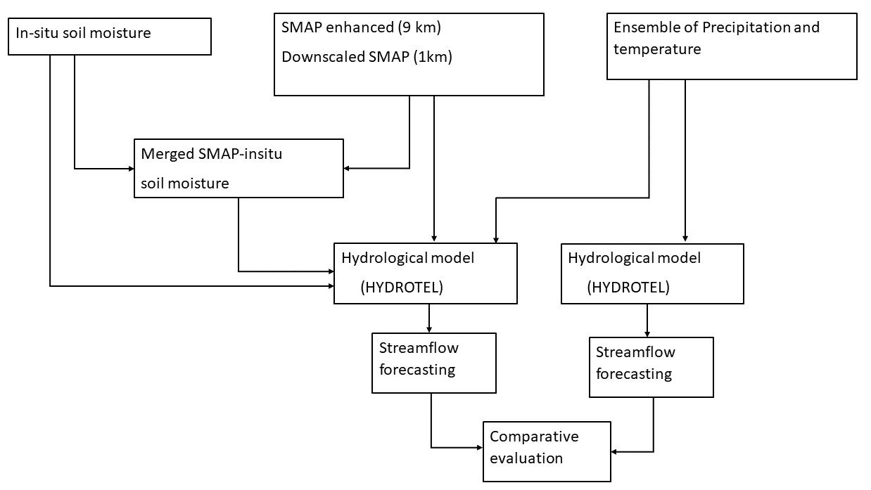
2.5. Model Updating with Soil Moisture

A set of experiments was implemented by updating the HYDROTEL model with the SMAP-enhanced (9 km), downscaled SMAP-enhanced (1 km), interpolated in-situ soil moisture and merged SMAP/in-situ soil moisture at 9 and 1 km for the streamflow forecasts. The updating was based on replacing the model top layer with SMAP, interpolated in-situ soil moisture or their merged versions, using the simplest data assimilation technique known as direct insertion [38]. The summary of implemented experiments is displayed in Figure 2.

Besides the model top layer, the intermediate layer (i.e., the second layer) of the model was updated by vertically extrapolated SMAP soil moisture using a semi-empirical approach called exponential filter [39]. This approach has a single parameter T (characteristics time length) which is used to indicate the temporal variability of soil moisture in the root zone profile and formulated as in Equation (3), and it was optimized by minimizing the RMSE value between the vertically extrapolated SMAP and deeper in-situ soil moisture (i.e., 20 cm).

$$SMr{z}_{tn}=SMr{z}_{tn-1}+K_n(SMsur{f}_{tn}-SMr{z}_{tn-1})$$

(3)

$$K_n=\frac{K_{n-1}}{K_{n-1}+exp\left(\frac{-1}{T}\right)}$$

(4)

where SMsurf and SMrz are surface and root zone soil moisture, T is the optimal characteristic decay time, tn is time step, and K is gain.

The model was updated with different SMAP, interpolated in-situ and merged SMAP/in-situ soil moisture prior to the forecasting issue day to represent the pre-storm soil moisture condition of the watershed. For example, for the forecast on 31 July, either the SMAP, interpolated in-situ soil moisture or merged SMAP/in-situ soil moisture on 30 July was used.

2.6. Validation of Downscaled and Merged SMAP/In-Situ Soil Moisture

In this study, the leave-one-out validation method was adopted to validate the merged SMAP/in-situ with in-situ soil moisture measurements. This method allows the use of 7 of 8 in-situ soil moisture stations available in the study area for interpolation, which then alternately merged with the SMAP soil moisture. In addition, the downscaled SMAP-enhanced and its original counterparts were validated with the in-situ soil moisture.

The classical statistical metrics, including the Pearson correlation coefficient (R) (Equation (5)), bias, (Equation (6)) and unbiased root mean square error (ubRMSE) (Equation (7)), were used to quantitatively evaluate the agreement between the merged SMAP/in-situ soil moisture against in-situ soil moisture observations. Similar calculations were used for the downscaled SMAP-enhanced and its original version.

$$\mathrm{R}=\frac{\sum \left({\mathsf{\theta }}_{\mathrm{DSM},\mathrm{i}}-{\overline{\theta }}_{DSM}\right)\left({\mathsf{\theta }}_{\mathrm{insitu},\mathrm{i}}-{\overline{\theta }}_{insitu}\right)}{\sqrt{\sum {\left({\mathsf{\theta }}_{\mathrm{DSM},\mathrm{i}}-{\overline{\theta }}_{DSM}\right)}^2{\left({\mathsf{\theta }}_{\mathrm{DSM},\mathrm{i}}-{\overline{\theta }}_{insitu}\right)}^2}}$$

(5)

$$RMSE=\sqrt{\frac{{\sum }_{i=1}^n{({\mathsf{\theta }}_{DSM}-{\mathsf{\theta }}_{insitu})}^2}{n}}$$

(6)

$$Bias=\frac{{\sum }_{i=1}^n{\mathsf{\theta }}_{DSM}-{\mathsf{\theta }}_{insitu}}{n}$$

(7)

$$ubRMSE=\sqrt{{\left(RMSE\right)}^2-{\left(bias\right)}^2}$$

(8)

2.7. Evaluation of Ensemble and Deterministic Streamflow Forecast Skills

The continuous ranked probability skill score (CRPSS) was used to evaluate the skill of the ensemble streamflow forecast [40]. This score has a value range between −∞ and 1. A score greater than zero indicates an improvement in ensemble streamflow forecast skill due to updating of the model with the SMAP or interpolated in-situ or the merged SMAP/in-situ soil moisture.

$$CRPSS=1-\frac{CRP{S}_{updated}}{CRP{S}_{non-updated}}$$

(9)

$$CRPS=\frac{1}{N}{\displaystyle \sum }_{i=1}^N\underset{-\infty }{\overset{\infty }{{\displaystyle \int }}}{\left[F_i\left(x\right)-F_i^0\left(x\right)\right]}^{2}dx$$

(10)

$$F^0\left(x\right)=\left\{\begin{array}{c}0, x\le observed streamflow value\\ 1, x>observed streamflow value\end{array}\right.$$

where the CRPS is the continuous ranked probability score, F_i(x) is the probability density function of the member of the ensemble simulation, and F⁰_i(x) is probability density function of observation.

The mean absolute error (MAE) was also used to calculate the accuracy of the deterministic forecast. The deterministic forecast is obtained by using the MSWEP precipitation and ERA-5 temperature of 2019. It is worth noting that we used the same data sources for calibration and validation of the model (see Section 2.2.3).

$$MAE=\frac{{\sum }_{i=1}^n\left|Q_{sim,i}-Q_{obs,i}\right|}{n}$$

(11)

where Q_sim and Q_obs are deterministic and observed streamflow, respectively, and n is the length of the time series.

In addition to the quantitative performance metrics, graphical comparison was made between the observed streamflow, deterministic forecast, ensemble forecast, and ensemble mean. Ensemble mean was obtained by averaging over all forecast members for each point in time.

3. Results

3.1. Model Performance Evaluation

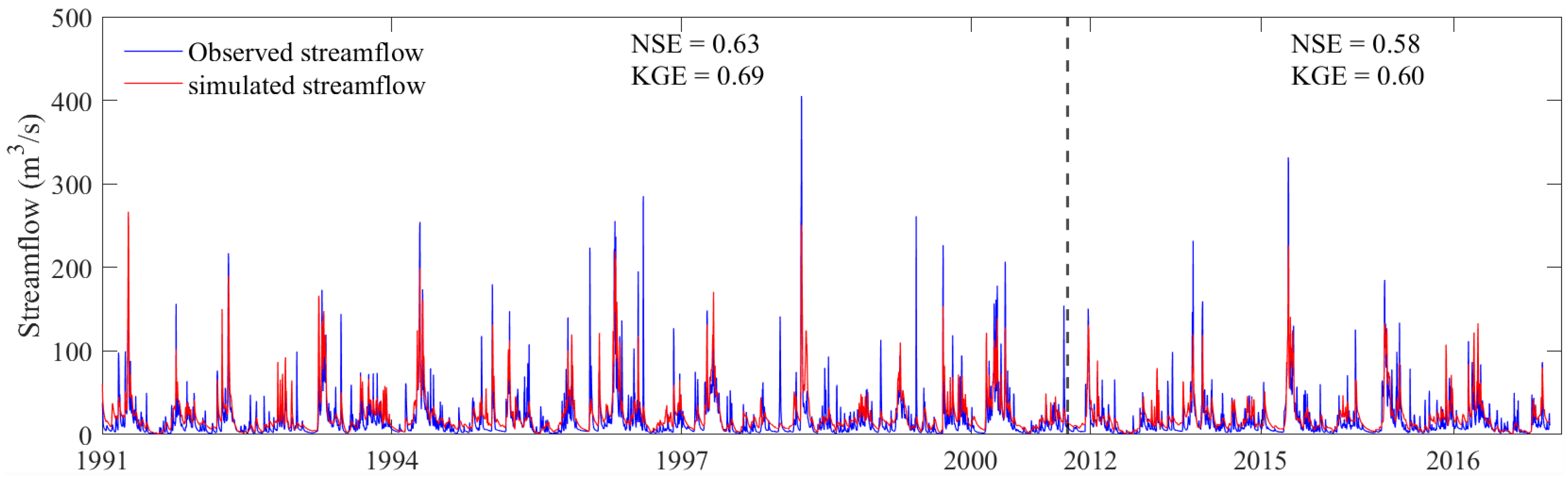
Figure 3 shows the comparison of observed and simulated hydrographs for a portion of calibration and validation periods to allow for clear presentation (i.e., to avoid overcrowding of the hydrographs in the figure). The qualitative inspection of the figure shows a good agreement between the simulated and observed hydrographs, except for overestimation or underestimation of some of the peak flows. In addition, the statistical metrics indicate a good model performance with NSE (KGE) values of 0.63 (0.69) and 0.58 (0.60) during calibration and validation periods, respectively.

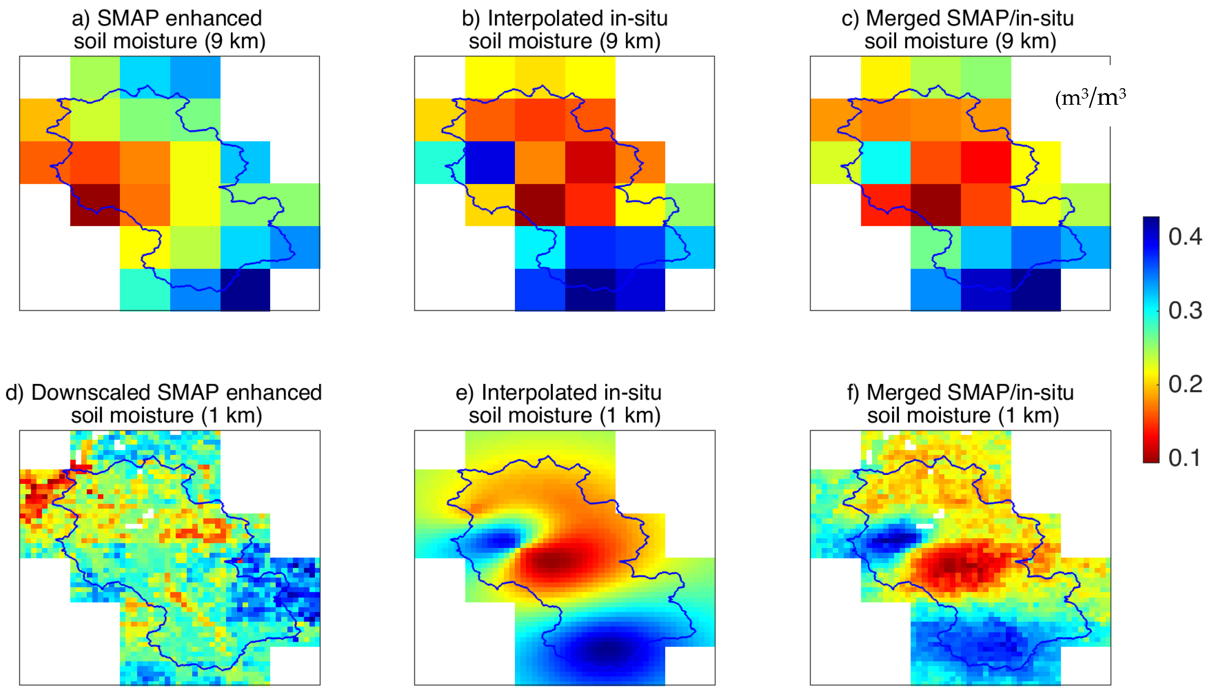
Figure 4 shows an example of maps of spatial distribution of SMAP-enhanced (i.e., both the original (9 km) and downscaled version (1 km)), interpolated in-situ soil moisture and the merged SMAP/in-situ soil moisture at 9 and 1 km resolutions on 8 August 2019. As can be observed in the figure, the 1 km downscaled SMAP-enhanced soil moisture (Figure 4d) brings out the fine-scale spatial heterogeneity of soil moisture over the au Saumon watershed compared to its original counterpart (Figure 4a). It also maintains the spatial pattern of its original counterpart (i.e., the original SMAP-enhanced soil moisture (9 km)). For example, the drier soil moisture condition of the original SMAP-enhanced soil moisture in the western part of the watershed is clearly reflected in downscaled SMAP-enhanced soil moisture.

The interpolated in-situ soil moisture maps over the au Saumon watershed at 9 and 1 km resolutions are shown in Figure 4b,e, respectively. Despite the small number of soil moisture probes and their uneven distribution in the watershed (see Figure 1), these maps somewhat exhibit a similar spatial pattern to that of the SMAP-enhanced soil moisture. For example, the maps of both SMAP-enhanced and interpolated in-situ measurements display a medium range of soil moisture at the top part of the watershed, while the center and lower parts are characterized by lower and higher soil moisture ranges, respectively.

On the other hand, the merged SMAP/in-situ soil moisture reasonably maintained the spatial patterns of SMAP-enhanced soil moisture, while keeping the accuracy of the interpolated in-situ soil moisture as can be seen in Figure 4c,f for the 9 and 1 km resolution, respectively.

3.2. Comparison of SMAP Soil Moisture, In-Situ and Merged SMAP/In-Situ Soil Moisture

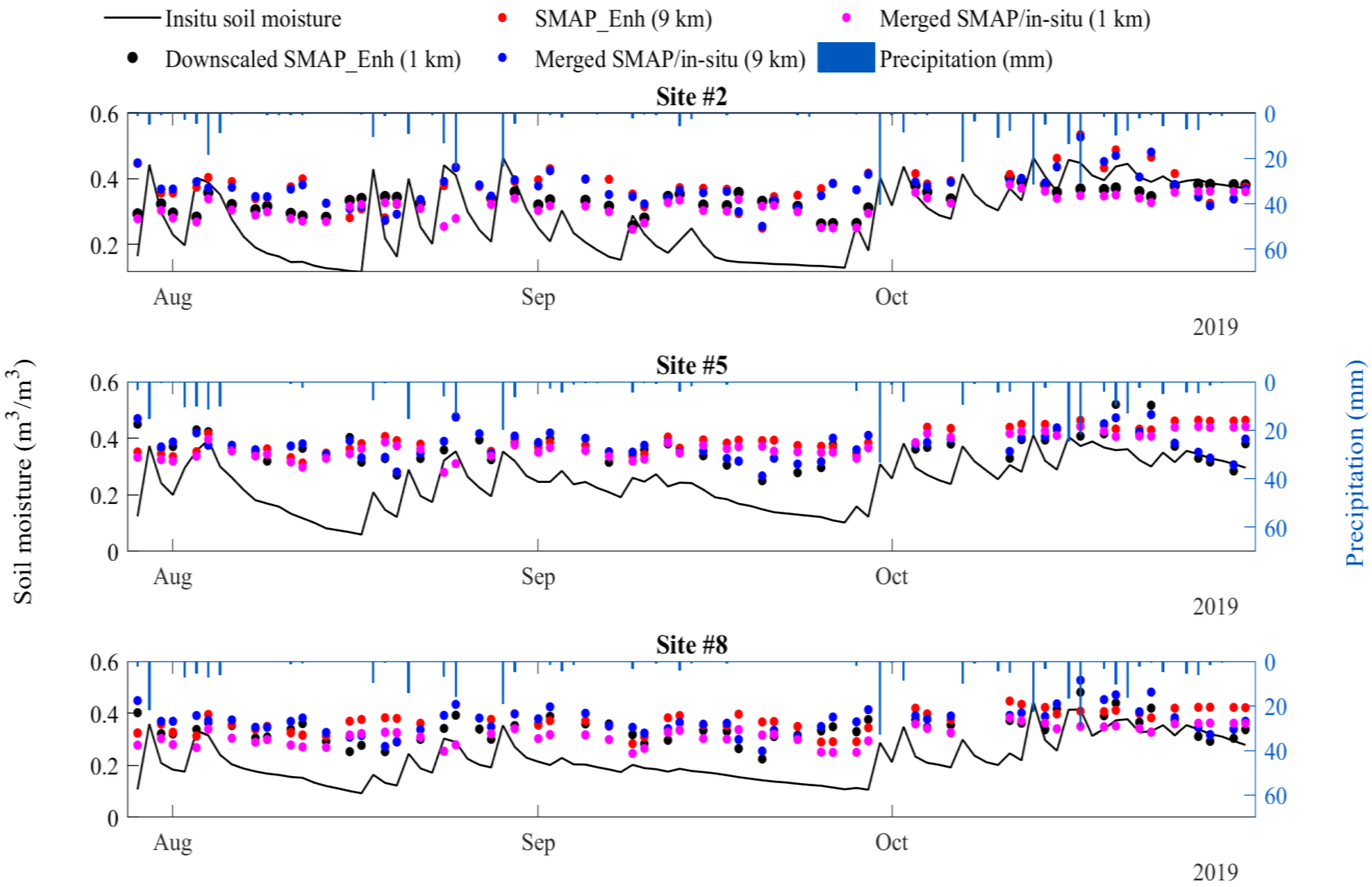
Figure 5 shows a time series comparison of the 1 km downscaled SMAP-enhanced and its original counterpart with the in-situ soil moisture measurements for selected locations in the au Saumon watershed from August to October of 2019. Both the original and downscaled SMAP-enhanced soil moisture reproduced the temporal dynamics of the in-situ soil moisture during wetter soil moisture conditions in late August and October reasonably well. However, during the drier soil moisture conditions, for example mid-August and mid to late October, both the original and downscaled SMAP overestimated soil moisture. Therefore, it can be inferred from the figure that the SMAP-enhanced reacts less to precipitation when compared to the in-situ soil moisture. This is because the forest cover in the au Saumon watershed interferes with the passive microwave signal emitted from the underlying soil. However, when compared to its original version, the 1 km downscaled SMAP-enhanced soil moisture tends to match better with the in-situ soil moisture, in particular when soil moisture is lower.

In addition, the figure also shows comparison of time series of the merged SMAP/in-situ soil moisture against in-situ measurements. Both the 9 and 1 km merged SMAP/in-situ soil moisture fairly reproduced the temporal variability of in-situ soil moisture. Compared to the 1 km downscaled SMAP, the 1 km merged SMAP/in-situ soil moisture better agrees with the in-situ soil moisture measurements. Similarly, the 9 km better matches the in-situ soil moisture than the original SMAP-enhanced soil moisture with a resolution of 9 km. However, overall, the SMAP tends to overestimate soil moisture compared to the in-situ soil moisture for all the three stations.

Besides the graphical comparison, performance metrics were used for quantitative evaluation.

Table 1. The performance metrics for SMAP-enhanced and merged SMAP/in-situ soil moisture.

Sites	SMAP and Merged SMAP/In-Situ Surface Soil Moisture
	Metrics	SMAP_Enh (9 km)	Downscaled SMAP_Enh (1 km)	Merged SMAP/In-Situ (9 km)	Merged SMAP/In-Situ (1 km)
Site #1	R	0.40	0.45	0.48	0.53
	ubRMSE	0.087	0.086	0.082	0.090
	Bias	0.087	0.084	0.097	0.077
Site #2	R	0.53	0.60	0.56	0.58
	ubRMSE	0.090	0.086	0.088	0.095
	Bias	0.110	0.092	0.106	0.084
Site #3	R	0.47	0.55	0.40	0.58
	ubRMSE	0.082	0.079	0.086	0.077
	Bias	0.049	0.090	0.065	0.088
Site #4	R	0.48	0.64	0.46	0.51
	ubRMSE	0.079	0.069	0.077	0.076
	Bias	0.149	0.147	0.145	0.138
Site #5	R	0.44	0.66	0.50	0.63
	ubRMSE	0.082	0.071	0.079	0.078
	Bias	0.031	0.033	0.034	0.025
Site #6	R	0.50	0.72	0.46	0.78
	ubRMSE	0.083	0.067	0.084	0.080
	Bias	0.173	0.206	0.194	0.194
Site #7	R	0.55	0.60	0.57	0.50
	ubRMSE	0.067	0.065	0.065	0.069
	Bias	0.163	0.142	0.158	0.137
Site #8	R	0.50	0.67	0.54	0.75
	ubRMSE	0.082	0.076	0.077	0.069
	Bias	0.048	0.030	0.055	0.015

shows a summary of quantitative performance of the SMAP and SMAP/in-situ soil moisture products at eight in-situ soil moisture stations in the au Saumon watershed. As can be seen in the table, the 1 km merged SMAP/in-situ soil moisture better agrees overall with the in-situ soil moisture with R values in a range of 0.5 to 0.78, ubRMSE values in a range of 0.069 to 0.095 m³/m³ and bias values in a range of 0.015 to 0.194 m³/m³ compared with the downscaled soil moisture with R values in a range of 0.45 to 0.72, ubRMSE values in a range of 0.065 to 0.086 m³/m³ and bias values in a range of 0.03 to 0.20 m³/m³. Similarly, the 9 km merged SMAP/in-situ soil moisture has a slightly better correlation with the in-situ soil moisture with R values in a range of 0.4 to 0.57 compared to SMAP-enhanced soil moisture (9 km) with R values in a range of 0.44 to 0.53.

3.3. Comparison of the Vertically Extrapolated SMAP/In-Situ and In-Situ Soil Moisture

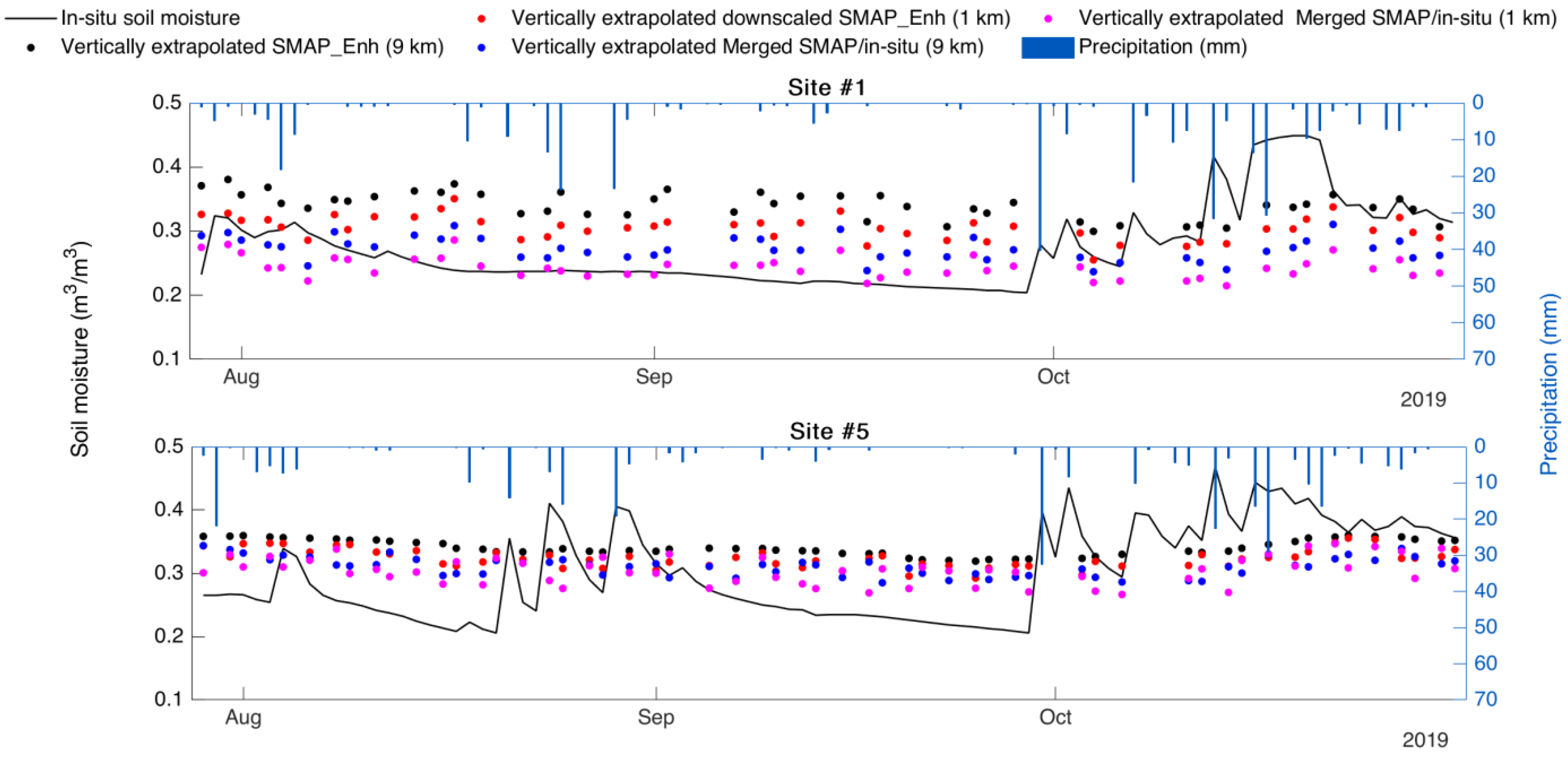
Figure 6 shows a comparison of the 1 km vertically extrapolated downscaled SMAP-enhanced soil moisture and its original counterpart (9 km) against in-situ soil moisture measured at a 20 cm depth. In addition, it also shows time series comparison of the merged vertically extrapolated SMAP/in-situ soil moisture at resolutions of 1 and 9 km against the in-situ soil moisture. The merged soil moisture products (i.e., at 1 and 9 km) better agree with in-situ soil moisture than their corresponding original SMAP component. Compared to the 9 km merged vertically extrapolated SMAP/in-situ soil moisture, the 1 km merged vertically extrapolated SMAP/in-situ soil moisture better matches with the temporal variability of in-situ soil moisture.

Moreover, the 1 km downscaled SMAP-enhanced, and its original counterparts generally overestimate in-situ soil moisture. The same holds true for their corresponding merged products. The vertical extrapolation also tends to smoothen the extrapolated soil moisture affecting its temporal dynamics. The obtained optimal T values vary across the in-situ soil moisture stations, yet their differences are not significant as the soil type (i.e., loamy soil) and land condition (i.e., forest dominated) of our watershed is similar. Thus, the T value varies between 17 and 21 days.

Quantitative comparison of vertically extrapolated SMAP and SMAP/in-situ with in-situ soil moisture at a 20 cm depth overall shows poor quantitative performance (

Table A1. The performance metrics for vertically extrapolated SMAP-enhanced and merged SMAP/in-situ soil moisture.

Sites	SMAP and Merged SMAP/In-Situ Vertically Extrapolated Soil Moisture
	Metrics	SMAP_Enh	Downscaled SMAP_Enh (1 km)	Merged SMAP/In-Situ (9 km)	Merged SMAP/In-Situ (1 km)
Site #1	R	0.33	0.33	0.34	0.45
	ubRMSE	0.15	0.16	0.16	0.18
	Bias	0.15	0.16	0.19	0.15
Site #3	R	0.38	0.40	0.28	0.50
	ubRMSE	0.15	0.15	0.17	0.15
	Bias	0.09	0.17	0.13	0.17
Site #4	R	0.39	0.47	0.32	0.44
	ubRMSE	0.14	0.13	0.15	0.15
	Bias	0.26	0.28	0.28	0.27
Site #7	R	0.45	0.44	0.40	0.43
	ubRMSE	0.12	0.12	0.13	0.14
	Bias	0.29	0.27	0.31	0.27
Site #8	R	0.41	0.49	0.38	0.64
	ubRMSE	0.15	0.14	0.15	0.14
	Bias	0.08	0.06	0.11	0.03

, Appendix A). However, the merged products still have slightly better performance compared to SMAP-enhanced soil moisture alone.

3.4. Updating the Model with the SMAP and In-Situ Soil Moisture

Figure 7 shows the comparison of the ensemble streamflow forecast with 15-days lead time between the non-updated (open-loop) and updated model with different soil moisture products, including the original SMAP-enhanced (9 km), downscaled SMAP-enhanced (1 km), and in-situ surface soil moisture. Three streamflow events were selected to examine the impact of updating the model with different soil moisture products on the accuracy of the ensemble streamflow forecast. Accordingly, the left panels show the ensemble streamflow forecast issued on 31 July 2019, whereas the middle and right panels show the forecast on 6 and 14 August 2019, respectively. Here, the updating was carried out only for the top layer of the model using the direct insertion assimilation technique.

As can be inferred from the figure, the ensemble streamflow forecast is improved by updating the model with the SMAP-enhanced (i.e., the original and downscaled) and in-situ surface soil moisture compared to the open loop. The ensemble mean (using EM-Earth product, shown in black) and the deterministic forecast (using MSWEP and ERA-5 land products, shown in red) agrees better with the observed streamflow, notably during the first few days of the forecast lead time. On the other hand, the ensemble spread increases when the model is updated with the SMAP soil moisture, while it is decreased when updated with in-situ soil moisture. This is probably because SMAP ‘sees’ higher soil moisture than in-situ measurements (see Figure 5 and Figure 6). In all cases, the ensemble generally better encompassed the observed streamflow, yet with the increase of the lead time, the ensemble spread becomes wider, as expected, resulting in the deterioration forecast accuracy.

When looking at the impact of the spatial resolution of SMAP-enhanced soil moisture on the accuracy of the ensemble streamflow forecast, updating the model with the 1 km downscaled SMAP-enhanced soil moisture resulted in a better ensemble streamflow forecast than when the model updated with its original counterpart (9 km). For example, for all three forecasts, the ensemble members better captured the observed streamflow when the model updated with the 1 km SMAP than its original counterpart. Similarly, the mean of the ensemble members and the deterministic forecast reasonably agree with the observed streamflow for the model updated with the 1 km SMAP-enhanced soil moisture product.

Similarly, updating the model with interpolated in-situ surface soil moisture improved the ensemble streamflow forecast, yet when compared to the 1 km downscaled SMAP-enhanced soil moisture, the improvement is less for the forecast on 31 July and 14 August 2019. However, for the forecast on 6 August 2019, the updating with the in-situ surface soil moisture produced a better forecast than the 1 km downscaled and original SMAP-enhanced soil moisture (9 km).

3.5. Updating the Model with the Merged SMAP/In-Situ Soil Moisture

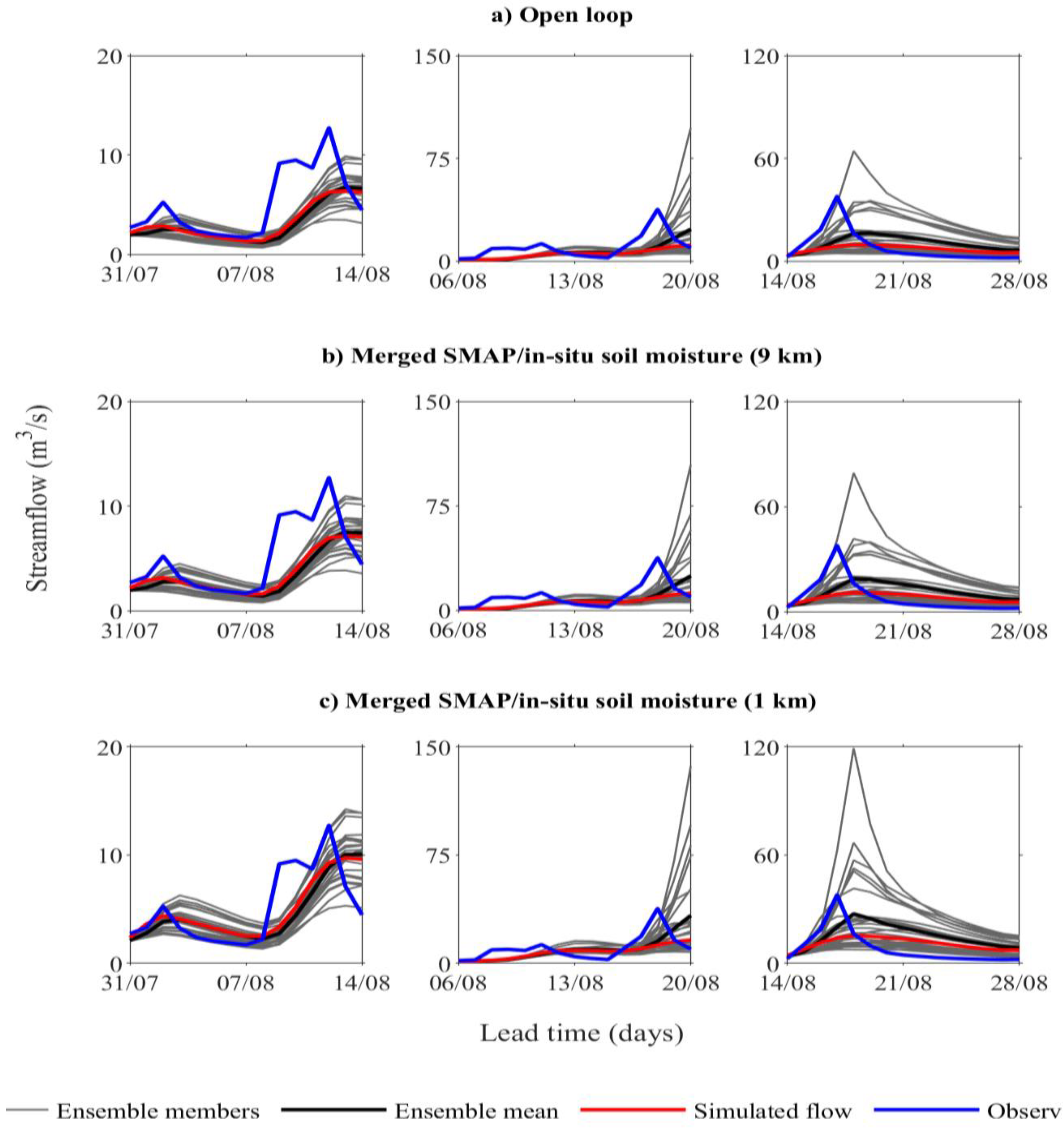
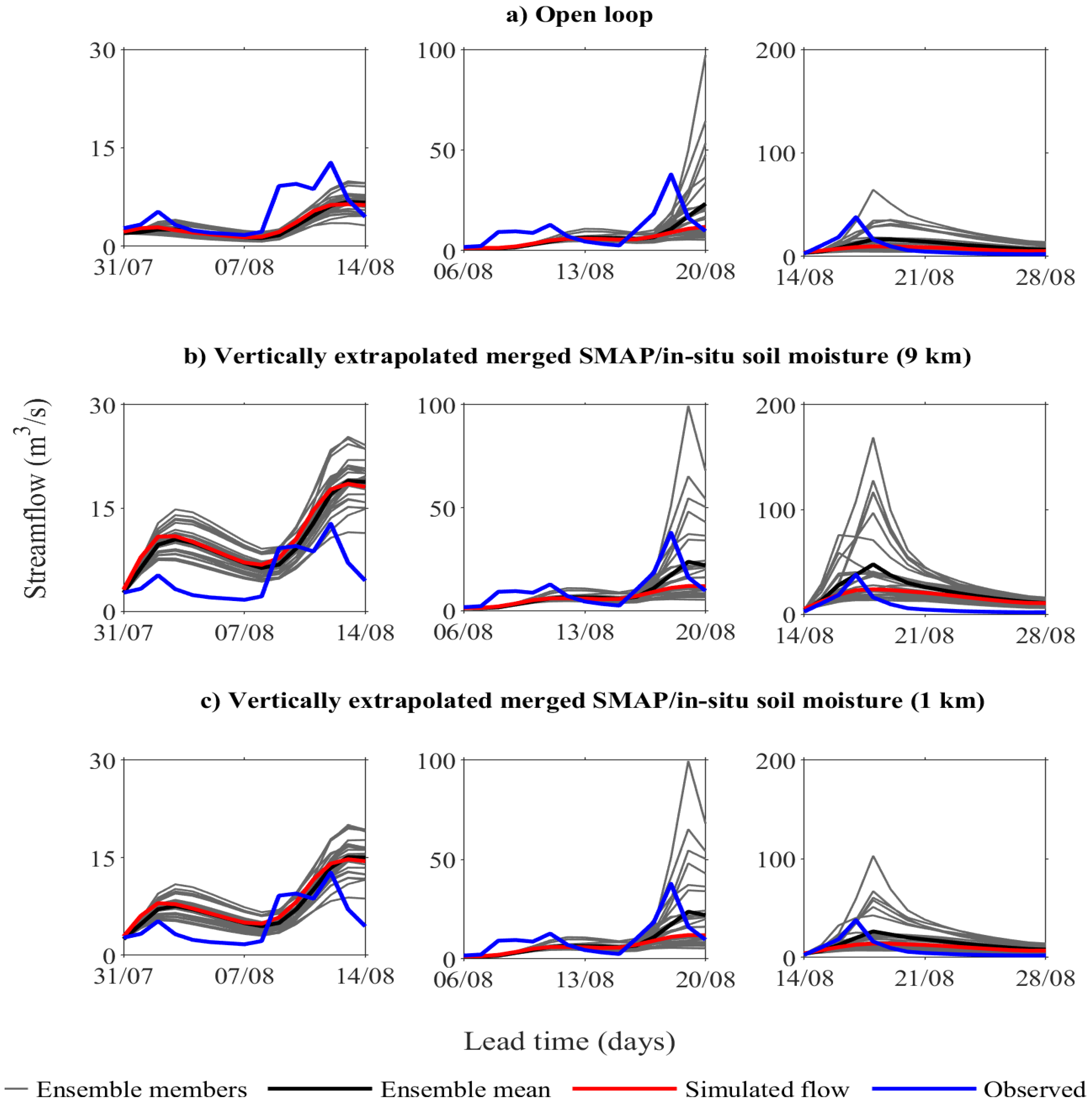
Figure 8 shows the comparison of the ensemble streamflow forecast between the model updated with the merged SMAP/in-situ soil moisture at 9 and 1 km spatial resolutions and the open loop. As can be observed from the figure, the ensemble streamflow forecast is improved when the model updated with merged SMAP/in-situ soil moisture both at 9 and 1 km spatial resolutions compared to the open loop. In addition, the ensemble mean and deterministic forecast closely agree with the observed streamflow, notably during the first few days of lead times, yet it tends to deteriorate with the increase of the lead time.

The ensemble members captured the observed streamflow better when the model updated with 1 km merged SMAP/in-situ soil moisture than when it updated with the 9 km merged SMAP/in-situ soil moisture. Likewise, the ensemble mean and the deterministic forecast agreed well with the observed streamflow for the 1 km merged SMAP/in-situ soil moisture. For example, for the forecast on 14 August, the observed streamflow falls outside of the ensemble members when the model updated with the 9 km merged SMAP/in-situ soil moisture, but when the model updated with the 1 km merged SMAP/in-situ soil moisture, the ensemble members shifted towards the observed streamflow.

On the other hand, the 1 km merged SMAP/in-situ soil moisture (Figure 8c) improved the ensemble streamflow forecast better than the model updated separately with either the 1 km downscaled SMAP (Figure 7c) or in-situ soil moisture (Figure 7d). However, the improvement was not that significant. For example, for the forecast on 14 August, the ensemble members are not able to capture the observed streamflow when updating the model with in-situ soil moisture alone, but when updating the model with the 1 km merged SMAP/in-situ soil moisture, the ensemble members shifted towards the observed streamflow.

3.6. Updating the Model with the Vertically Extrapolated SMAP Soil Moisture

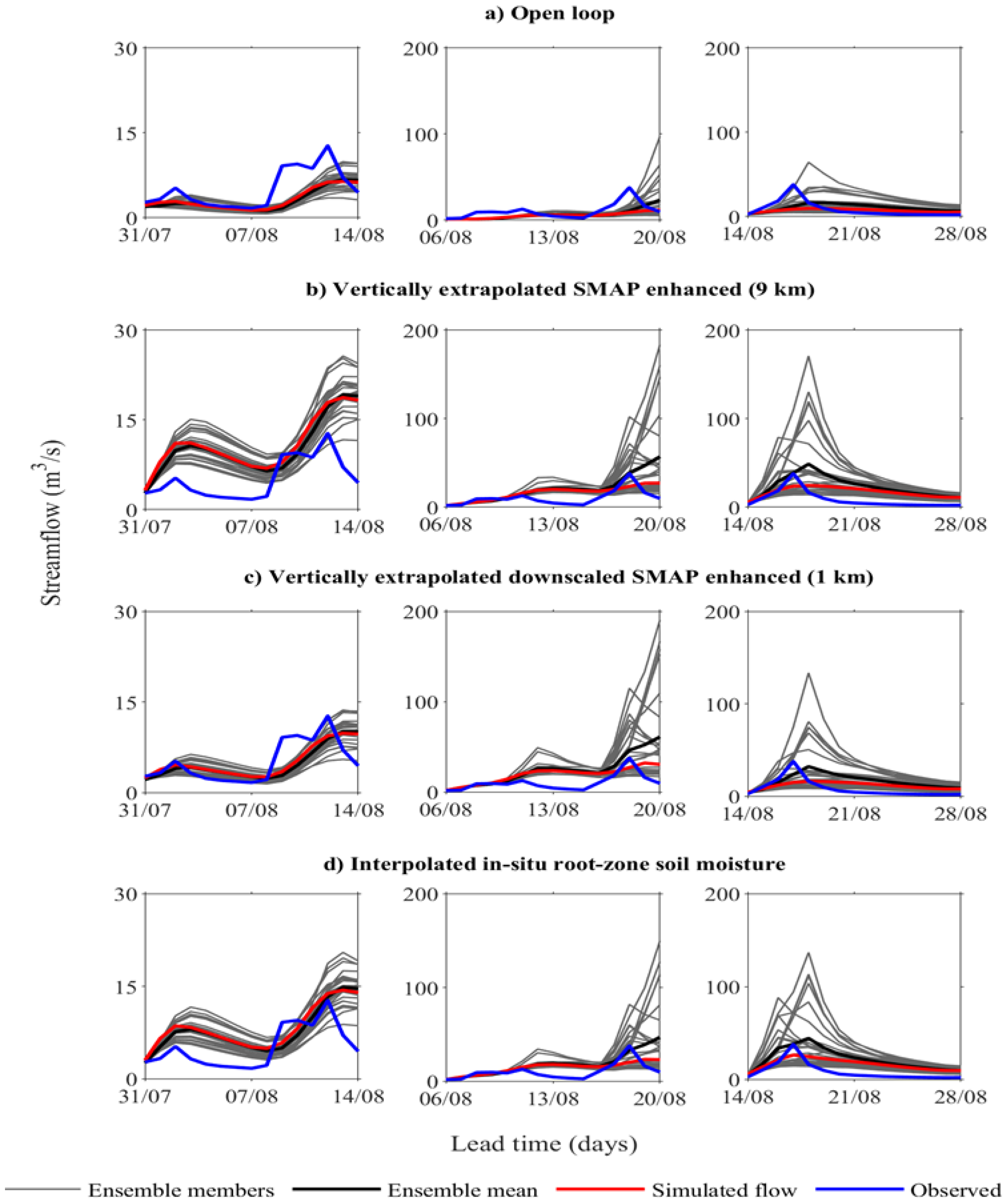
Figure 9 shows the ensemble streamflow forecast after updating top and intermediate layers of the model with surface and vertically extrapolated SMAP-enhanced soil moisture, respectively. In addition, the ensemble streamflow forecast for the model updated with surface and subsurface (rootzone) in-situ soil moisture is shown in Figure 9d. Compared to the open loop (Figure 9a), updating the top and intermediate layers of the model (Figure 9b,c) moderately improved the overall ensemble streamflow forecasts with the exception of the forecast on 31 July 2019, which overestimated the ensemble streamflow forecast when the model updated with the vertically extrapolated original SMAP-enhanced soil moisture (9 km). The ensemble mean and the deterministic forecast closely match the observed streamflow, notably during the first few days of lead time for all forecasts (Figure 9b). In general, updating the top and intermediary layers increased the forecasted streamflow.

When looking at the impact of spatial resolution, updating the model with the 1 km downscaled SMAP-enhanced vertically extrapolated soil moisture produced better ensemble streamflow forecast than when the model updated with its coarser counterpart or subsurface in-situ soil moisture. For example, for the forecast on 31 July the ensemble members were able to capture the observed streamflow when the model updated with the 1 km vertically extrapolated SMAP-enhanced soil moisture, yet updating the model with the 9 km vertically extrapolated SMAP-enhanced soil moisture overestimated the ensemble streamflow forecast.

Moreover, updating the top and intermediate layers of the model with in-situ surface and subsurface soil moisture (Figure 9d), respectively, resulted in overestimation of the ensemble streamflow forecast compared to that of the open loop and the model updated with the 1 km vertically extrapolated downscaled SMAP-enhanced soil moisture for the forecast on 31 July 2019.

3.7. Updating the Model with the Vertically Extrapolated SMAP/In-Situ Soil Moisture

Figure 10 shows the comparison of ensemble streamflow forecast between the open loop and the updated model with the vertically extrapolated merged SMAP/in-situ soil moisture at 9 and 1 km spatial resolutions. Compared to the open loop, updating the model with the 9 km vertically extrapolated merged SMAP/in-situ soil moisture slightly improved the streamflow forecast on 6 August 2019, whereas the forecast on 31 July and 14 August were overestimated. On the other hand, the assimilation of the 1 km vertically extrapolated SMAP/in-situ soil moisture resulted in a better ensemble streamflow forecast for the forecast on 6 and 14 August, yet the forecast on 31 July was still overestimated, but to a lesser extent compared with the assimilation of the 9 km product.

When looking at the impact of spatial resolution, the ensemble streamflow forecast by the model updated with the 1 km vertically extrapolated merged soil moisture generally outperformed the one updated with the 9 km vertically extrapolated merged SMAP/in-situ soil moisture. For example, for the forecast on 31 July, the model updated with the 9 km vertically extrapolated merged soil moisture considerably overestimated the streamflow forecast compared to the model updated with 1 km vertically extrapolated merged SMAP/in-situ soil moisture.

3.8. Comparison between Experiments

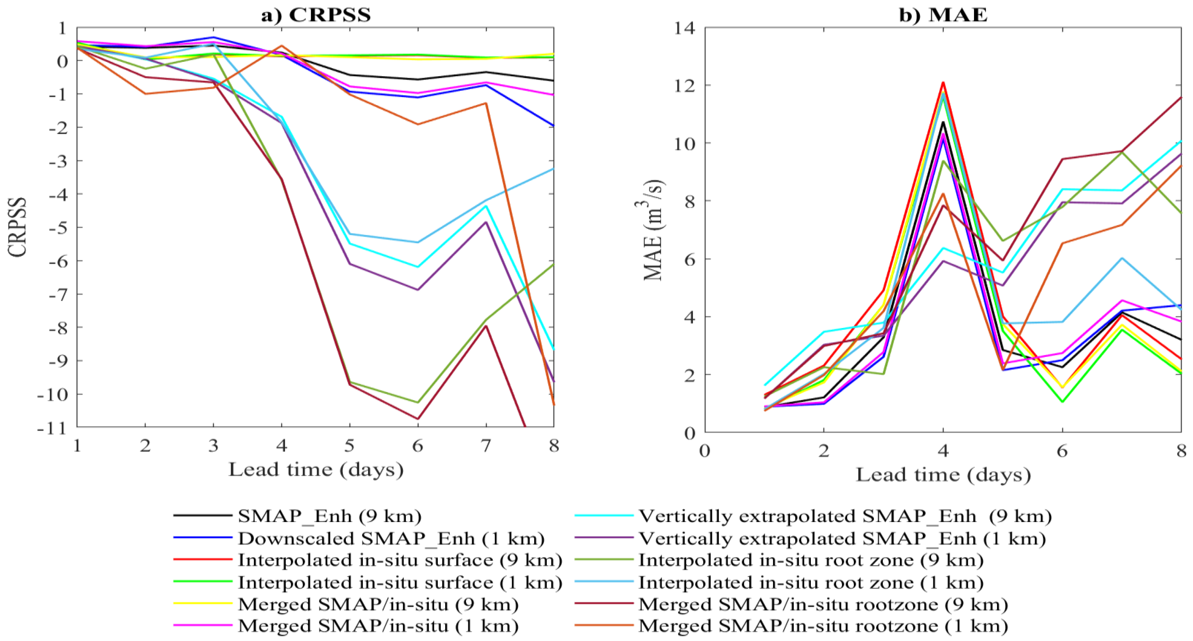
Figure 11a shows the mean CRPSS (MCRPSS) values with respect to lead time for different soil moisture products. The MCRPSS was averaged over the three forecast cases (forecast on 31 July, 6 August and 14 August) for each lead day. As can be seen in the figure, the MCRPSS decreases with the lead time for all soil moisture products. Put differently, the forecast skill is higher during the first few days of the lead time for all soil moisture products. Similarly, the MAE for the deterministic forecast is lower during the first few days of lead time (Figure 11b).

When comparing different soil moisture products, the assimilation of 1 km merged SMAP/in-situ soil moisture, the 1 km downscaled soil moisture and the 9 km merged SMAP/in-situ soil moisture improved the streamflow forecast skills as indicated by higher CRPSS and lower MAE both for ensemble and deterministic forecasts, respectively. On the other hand, the vertically extrapolated soil moisture products, including vertically extrapolated SMAP (9 km), interpolated in-situ rootzone soil moisture and the 9 km vertically extrapolated merged SMAP/in-situ soil moisture, deteriorated the streamflow forecast skills both for the ensemble and deterministic forecasts.

4. Discussion

The downscaled SMAP-enhanced soil moisture (1 km) reflected the spatial detail of soil moisture over the au Saumon watershed well, while maintaining the spatial pattern of the original SMAP-enhanced soil moisture (9 km). However, the SMAP-enhanced soil moisture (i.e., both the downscaled and original) reacted less to precipitation and tended to overestimate soil moisture when compared to the in-situ measurements, notably during dry conditions. This is primarily because of the sub-optimal quality of SMAP soil moisture retrievals over a forested watershed like ours, and this is ascribed to the weak penetration of SMAP through a dense vegetation canopy [5,41]. Over such an area, both soil surface and vegetation emission contribute to the received signal by the SMAP radiometer, and it is complicated to decouple the contribution of both the vegetation and soil surface.

The merging of the SMAP-enhanced and in-situ soil moisture resulted in improved maps of soil moisture by maintaining the spatial heterogeneity of SMAP-enhanced soil moisture while preserving the dynamic range of in-situ of soil moisture. This agreed with the study by Kim et al. [42] who merged AMSR2 soil moisture with in-situ measurements over the Korean Peninsula.

Updating the top layer of the model with the merged SMAP/in-situ soil moisture improved the accuracy of the ensemble streamflow forecast compared to the open loop. However, the level of improvement varied with the resolution of merged SMAP/in-situ soil moisture. Overall, the 1 km merged SMAP/in-situ soil moisture resulted in a better ensemble streamflow forecast than the 9 km merged SMAP/in-situ soil moisture. This is because the 1 km resolution better reflects the spatial detail of soil moisture. This is in line with previous studies which showed the importance of higher-resolution satellite soil moisture assimilation for improving the streamflow simulation [17,23], yet the assimilation of merged satellite/in-situ soil moisture, to the best of our knowledge, is very rare for comparison to our study.

In another experiment, updating the top layer of the model with in-situ soil moisture alone (Figure 6d) resulted in less improvement in the accuracy of the ensemble streamflow forecast than the merged SMAP/in-situ soil moisture product for some of the forecasts (Figure 7b,c). For example, the CRPSS value was reduced from 0.230 to 0.120 for the ensemble forecast on 6 August. On the other hand, the MAE reduced from 1.98 to 1.90 m³/s and from 4.52 to 4.28 m³/s for the deterministic forecasts on 31 July and 6 August, respectively. This was mainly because of a very low density of in-situ soil moisture probes, which cannot sufficiently reflect the spatial variability of soil moisture in the au Saumon watershed. Our finding is not in line with the study conducted on the Little Washita River experimental watershed where assimilation of in-situ soil moisture significantly improved the streamflow forecasting [43]. This was mainly because there is a high spatial density of in-situ soil moisture measurements in the Little Washita Watershed compared to the au Saumon watershed, which adequately represents the spatial variability of soil moisture in the watershed.

Similarly, updating the top layer of the model with SMAP-enhanced soil moisture (i.e., either the downscaled or original) alone resulted in less improvement in the accuracy of the ensemble streamflow forecast compared to updating with the merged SMAP/in-situ soil moisture. This is primarily because of the lower quality of SMAP-enhanced soil moisture retrievals over the au Saumon watershed. This watershed is heavily forested, which in turn affected the quality of the SMAP soil moisture retrieval as stated before. Because of that, the SMAP tends to overestimate soil moisture and the assimilation of this wet bias tends to reduce the skill of the ensemble streamflow forecast. This agrees with the study by Abbaszadeh et al. [17] which reported less accurate model predictions due to the assimilation of overestimated SMAP soil moisture because of the presence of lakes in part of their study area which affected the quality of the SMAP soil moisture retrieval.

Additional experiments were also conducted to investigate the impact of updating the intermediate (i.e., the second) layer of the model in addition to the top layer. The top and intermediate layers of the model were updated with the surface and vertically extrapolated merged SMAP/in-situ soil moisture, respectively. Updating both layers of the model deteriorated the accuracy of the ensemble streamflow forecast. Similarly, updating either with the vertically extrapolated SMAP-enhanced or subsurface in-situ soil moisture alone did not improve the ensemble streamflow forecast.

This might be partly attributed to the addition or removal of water to the soil when updating the second layer of the model, which is then redistributed by the model subsequently affecting the streamflow generation. In addition, the coupling strength between the top and second layers of the model could affect the accuracy of the ensemble streamflow forecast. The coupling between the two layers depends on many factors, including vegetation, soil properties and climate conditions [44]. For example, the dominance of vegetation in the au Saumon watershed reduces the exposure of the ground surface to atmospheric conditions and is expected to result in strong coupling between the surface and subsurface soil moisture. However, the expected strong coupling between the top and second layers of the model did not bring improvement in the accuracy of ensemble streamflow forecasts. This might be due to the subsurface physics of HYDROTEL, which was not explicitly designed to take into account the vertical coupling between the top and second layers of the model.

Overall, the gain in the accuracy of the ensemble streamflow forecast when the model updated with the merged SMAP/in-situ soil moisture is not that significant compared to when the model separately updated either with SMAP-enhanced or in-situ soil moisture. This could be attributed to the quality of the merged SMAP/in-situ soil moisture, which in turn depends on the quality of the SMAP-enhanced soil moisture and in-situ soil moisture. The spatial interpolation of in-situ soil moisture was affected by the paucity of in-situ probes in the au Saumon watershed, while the quality of the SMAP-enhanced soil moisture retrieval was affected by the presence of vegetation as previously discussed. These weaknesses of SMAP and in-situ soil moisture propagates into the merged SMAP/in-situ soil moisture, thereby affecting the accuracy of the ensemble streamflow when updating the model.

5. Conclusions

The L-band passive microwave satellites (e.g., the SMOS and SMAP) and in-situ measurements are established methods for estimation of soil moisture. Over the au Saumon watershed, which is dominated by forests, SMAP overestimated soil moisture and reacted less to precipitation, while in-situ measurements reacted well to precipitation, producing a better dynamic range of soil moisture. On the other hand, SMAP reproduced the spatial distribution of soil moisture better than in-situ measurements. This is because the in-situ measurements are not adequate to capture the spatial variability of soil moisture there are few probes over the au Saumon watershed. This highlights the importance of combining the strength of SMAP and in-situ soil moisture to generate soil moisture with better quality while compensating for their respective weaknesses. Thus, the conditional merging technique was adopted for this purpose.

The merging of SMAP-enhanced soil moisture with the in-situ measurements improved the spatio-temporal representation of soil moisture over the au Saumon watershed compared with any single one of them by preserving the spatial variability of SMAP and the dynamic range of in-situ soil moisture. The 1 km merged SMAP/in-situ soil moisture represented the spatial detail of soil moisture better than the 9 km merged SMAP/in-situ soil moisture.

The assimilation of the merged SMAP/in-situ surface soil moisture overall improved the accuracy of the ensemble streamflow forecast compared to when they were used separately. However, the additional improvement obtained by using the merged SMAP/in-situ soil moisture was not that significant when compared to using the model separately updated either with the SMAP-enhanced or in-situ soil moisture alone. On the other hand, when comparing in terms of spatial resolution, the 1 km merged SMAP/in-situ soil moisture produced a reasonably better ensemble streamflow forecast than the 9 km merged SMAP/in-situ soil moisture.

The assimilation of the vertically extrapolated merged SMAP/in-situ soil moisture did not bring further improvement to the accuracy of the ensemble streamflow forecast compared to the open loop. This remains true when the model was separately updated with the vertically extrapolated SMAP-enhanced and subsurface in-situ soil moisture alone.

Besides its contributions, this study also has some limitations which are worth mentioning. First, the au Saumon watershed is heavily forested, which subsequently affects the quality of the SMAP soil moisture retrievals. Second, the number of in-situ soil moisture measurement probes are not adequate to represent the spatial variability of soil moisture in the au Saumon watershed. Hence, the lack of spatially dense in-situ soil moisture measurement stations along with the sub-optimal quality of the SMAP soil moisture affects the quality of the merged SMAP/in-situ soil moisture. This consequently affects the accuracy of ensemble streamflow forecast when assimilated.

In future studies, the merging of different satellite soil moisture products with in-situ soil moisture is encouraged. There are several networks of in-situ soil moisture measurements with different densities across the globe. Exploring the impact of the density of these networks on the merging with satellite soil moisture and thereby on the accuracy of streamflow forecasting would be interesting.

Exploring different merging techniques is also a good perspective to consider. In addition, the use of real ensemble meteorological forecast for forcing a hydrological model is encouraged while assimilating the merged satellite/in-situ soil moisture. Finally, exploring more advanced data assimilation schemes along with merged products is also encouraged.

In addition, merging the merged satellites passive microwave soil moisture (e.g., SMAP and SMOS) with the in-situ soil moisture would be worth exploring.