Suspended Sediments in Environmental Flows: Interpretation of Concentration Profiles Shapes

Abstract

In environmental flows, field and laboratory measurements of suspended sediments show two kinds of concentration profiles. For coarse sediments, a near-bed upward convex profile is observed beneath the main upward concave profile. In this study, we consider two 1-DV models, namely, the classical advection–diffusion equation (ADE) based on the gradient diffusion model, and the kinetic model. Both need sediment diffusivity, which is related to the eddy viscosity, and an y-dependent β-function (i.e., the inverse of the turbulent Schmidt number). Our study shows that the kinetic model reverts to the classical ADE with an “apparent” settling velocity or sediment diffusivity. For the numerical resolution of the ADE, simple and accurate tools are provided for both the sediment diffusivity and hindered settling. The results for the concentration profiles show good agreement with the experimental data. An interpretation of the concentration profiles is provided by two “criteria” for shapes. The main for steady open-channel flows shows that the shape of the concentration profiles in the Cartesian coordinate depends on the vertical distribution of the derivative of $R$ (the ratio between the sediment diffusivity and the settling velocity of the sediments): dR/dy > −1 for the upward concave concentration profile while dR/dy < −1 for the near-bed upward convex profile. A generalization is proposed for oscillatory flows over sand ripples, where the time-averaged concentration profiles in the semi-log plots are interpreted by a relation between the second derivative of the logarithm of the concentration and the derivative of the product between the sediment diffusivity and an additional parameter related to the convective sediment entrainment process.

1. Introduction

Accurate prediction of the concentration profiles for suspended sediments presents an important field of research due to its implication in different practical applications in both river and costal engineering [1,2,3,4,5,6,7,8,9,10,11,12,13,14,15]. Careful examination of field and laboratory experimental data show two kinds of concentration profiles depending on particles size (i.e., upward convex/concave profiles for fine/coarse sediments) [16,17,18,19,20,21,22]. Most modeling studies use the widely and well-known approach based on the gradient diffusion model. The resolution of the related classical one-dimensional vertical (1-DV) advection-diffusion equation (ADE) needs the sediment diffusivity ${\epsilon }_s$ and the settling velocity of sediments ${\omega }_s$. The diffusivity of sediments ${\epsilon }_s$ is related to the diffusivity of momentum, i.e., the eddy viscosity ${\nu }_t$, by a coefficient $\beta ={\epsilon }_s/{\nu }_t$ (i.e., the inverse of the turbulent Schmidt number).

In rivers and open-channel flows, laboratory experiments were conducted for fully developed steady uniform flow conditions in order to obtain more knowledge about the involved physics related to suspended sediments. While for fine sediments the data exhibit upward concave profiles, for coarse sediments a near-bed upward convex profile is observed beneath the main upward concave profile [16,17]. Examination of the well-known analytical solution of the ADE i.e., the Rouse formula [23], by experimental data of suspended sediment concentrations [16] shows that for fine sediments, the upward concave profiles are well described by the ADE with adequate formulations for the eddy viscosity and β-factor. However, for coarse sediments, the ADE fails to predict the near-bed upward convex profile [17]. Based on a fall velocity that varies according to the grain Reynolds number, Umeyama [24] divided the concentration field into an outer region and an inner region and proposed two formulas for each region. The ADE was often used with β equal to 1 and a constant sediment settling velocity equal to the terminal settling velocity of a particle alone in an infinite fluid. In this case, the predicted concentration profiles, which depend only on the eddy viscosity model, fail to predict the near-bed measured concentrations. In particular, errors appear in the concentration distribution for flows with coarse sediments and/or high concentrations.

In order to improve the suspended sediment concentrations models, two kinds of research were conducted. On the one hand, studies were conducted to improve the description of the parameters involved in the ADE. Equations for β have been proposed [25,26], and c-dependent [27] and y-dependent [22] β-functions have been introduced. The well-known equation of Richardson and Zaki [28] for the sediment settling velocity ${\omega }_s$ has been considered. On the other hand, these errors were related to a weakness in the ADE and dispersion mechanisms that were not accounted in the ADE [17] that was considered as unable to predict the near-bed concentration profiles for flows with coarse sediments and/or high concentrations. The kinetic model was used in order to improve results from the ADE [17] thanks to the effect of the lift force and the sediment stress gradient. Results from the kinetic model showed good agreement with experimental data and were related to the sediment stress gradient, which was found to be significant for a relative flow depth below 0.1.

The aim of this study is to provide explanations and tools about the modeling of the near-bed concentration profile for coarse sediments by the ADE for suspended sediments in both open-channel flows and oscillatory flows over sand ripples. In Section 2, two models of suspended sediment concentrations, given by two ordinary differential equations (ODE), are presented as follows: the classical advection–diffusion equation based on the gradient diffusion model and the kinetic model. Both models need the sediment diffusivity, which is the key parameter in suspended sediment concentration modeling. Section 3 is therefore dedicated to the analytical modeling of the sediment diffusivity. Section 4 is for suspended sediments in steady uniform open-channel flows while Section 5 is for suspended sediments in oscillatory flows over sand ripples.

2. Mathematical Modeling of Suspended Sediment Concentrations

2.1. Classical Advection–Diffusion Equation Based on the Gradient Diffusion Model

In equilibrium conditions, the concentration of the suspended sediment results from the balance between an upward mixing flux $q_m$ and a downward settling flux $q_s=c\left(y\right) {\omega }_s$ as $q_m-c\left(y\right) {\omega }_s=0$, where ${\omega }_s$ is the particle settling velocity and $y$ the vertical distance from the bed. The gradient diffusion model assumes that the mixing flux is proportional to the concentration gradient $q_m=-{\epsilon }_s\frac{dc}{dy}$; where ${\epsilon }_s$ is the sediment diffusivity and makes it possible to write the classical 1-DV advection–diffusion equation (ADE) as

$${\epsilon }_s\frac{dc}{dy}+{\omega }_{s}c=0$$

(1)

2.2. The Kinetic Model

The kinetic model for turbulent two-phase flows accounts for both particle–turbulence interactions and particle–particle collisions. In turbulent solid–liquid flows, these models use the Lagrangian equations of particle dynamics. The kinetic model deals with passing from the Lagrangian equation to the Eulerian ones though a stochastic description. The method of moments is used in order to simplify the equations.

In this model, for passing from the Lagrangian equations to the Eulerian ones, a probability density distribution function (PDF) for particles is introduced. Through differentiating this function with respect to time $t$, a closed kinetic equation is obtained.

With the assumptions related to two-dimensional, fully developed, steady open-channel flows, the sediment $y$-momentum equation is written as [17]

$${\epsilon }_s\frac{dc}{dy}+{\omega }_{s}c-c {\tau }_p\left(F_L+F_{syns}\right)=0,$$

(2)

where ${\tau }_p$ is the particle relaxation time, $F_L$ the lift force acting on the particles and $F_{syns}$ a force produced by the gradient of sediment $y$ direction normal stress. In Equation (2) the sediment diffusivity ${\epsilon }_s$ is equal to ${\epsilon }_{pd}+\left({\nu }_t/\left(1+St\right)\right)$ [17], where ${\epsilon }_{pd}$ is the drift–diffusion coefficient and $St$ the particle Stokes number.

2.3. Improved Advection–Diffusion Equations

Both ordinary differential Equations (ODE) (1) and (2) need the sediment diffusivity and the settling or fall velocity which are the key parameters in suspended sediment concentration modeling. Section 3 is dedicated to the analytical modeling of the sediment diffusivity. Equation (2) introduces an additional correction term to the classical ADE (1). This additional term from the kinetic model in Equation (2) is similar to a hindered settling effect. In Section 4, we will show that Equation (2) reverts to the classical ADE (1) with an “apparent” settling velocity or “apparent” sediment diffusivity.

3. Sediment Diffusivity

The diffusivity of sediments ${\epsilon }_s$ is related to the diffusivity of momentum, i.e., the eddy viscosity ${\nu }_t$, by a coefficient $\beta$. The sediment diffusivity is given therefore by

$${\epsilon }_s=\beta {\nu }_t,$$

(3)

where the $\beta$-factor is the inverse of the turbulent Schmidt number.

In this section, analytical methods are proposed for both the eddy viscosity and $\beta$-factor (i.e., the inverse of the turbulent Schmidt number).

3.1. Eddy Viscosity

In engineering applications, the eddy viscosity is the main parameter related to turbulence. Suitable analytical eddy viscosity models are based on the concepts of velocity and length scales [29,30,31]. In these models, the eddy viscosity is given by the product of a mixing length $l_m$ and a mixing velocity $w_m$ [32,33,34] which is related to the exponentially decreasing turbulent kinetic energy (TKE) function. This method provides the exponential-type profile of the eddy viscosity [34] given by

$${\nu }_t\left(y\right)=u_{*}y{e}^{-\frac{y^{+}+0.34{Re}_{*}-11.5}{0.46{Re}_{*}-5.98}},$$

(4)

where in wall units $y^{+}=y{u}_{*}/\nu$, ${Re}_{*}=h{u}_{*}/\nu$ is the friction Reynolds number, $u_{*}$ the friction or shear velocity, $\nu$ the kinetic viscosity and $h$ the flow depth.

This $R{e}_{*}$-dependent eddy viscosity (4) was validated through the computation of the velocity profiles and the comparisons to the experimental data of both the velocities and the eddy viscosity [34]. It is possible to write Equation (4) in the following form

$${\nu }_t\left(\xi \right)=C_{\mathsf{\alpha }} u_{*}y{e}^{-C_1\xi },$$

(5)

where $\xi =y/h$ and the two coefficients $C_{\mathsf{\alpha }}$ and $C_1$ are given by [34]

$$C_{\mathsf{\alpha }}=e^{-\frac{0.34{Re}_{*}-11.5}{0.46{Re}_{*}-5.98}}\mathrm{and}{C}_1=\frac{{Re}_{*}}{0.46{Re}_{*}-5.98},$$

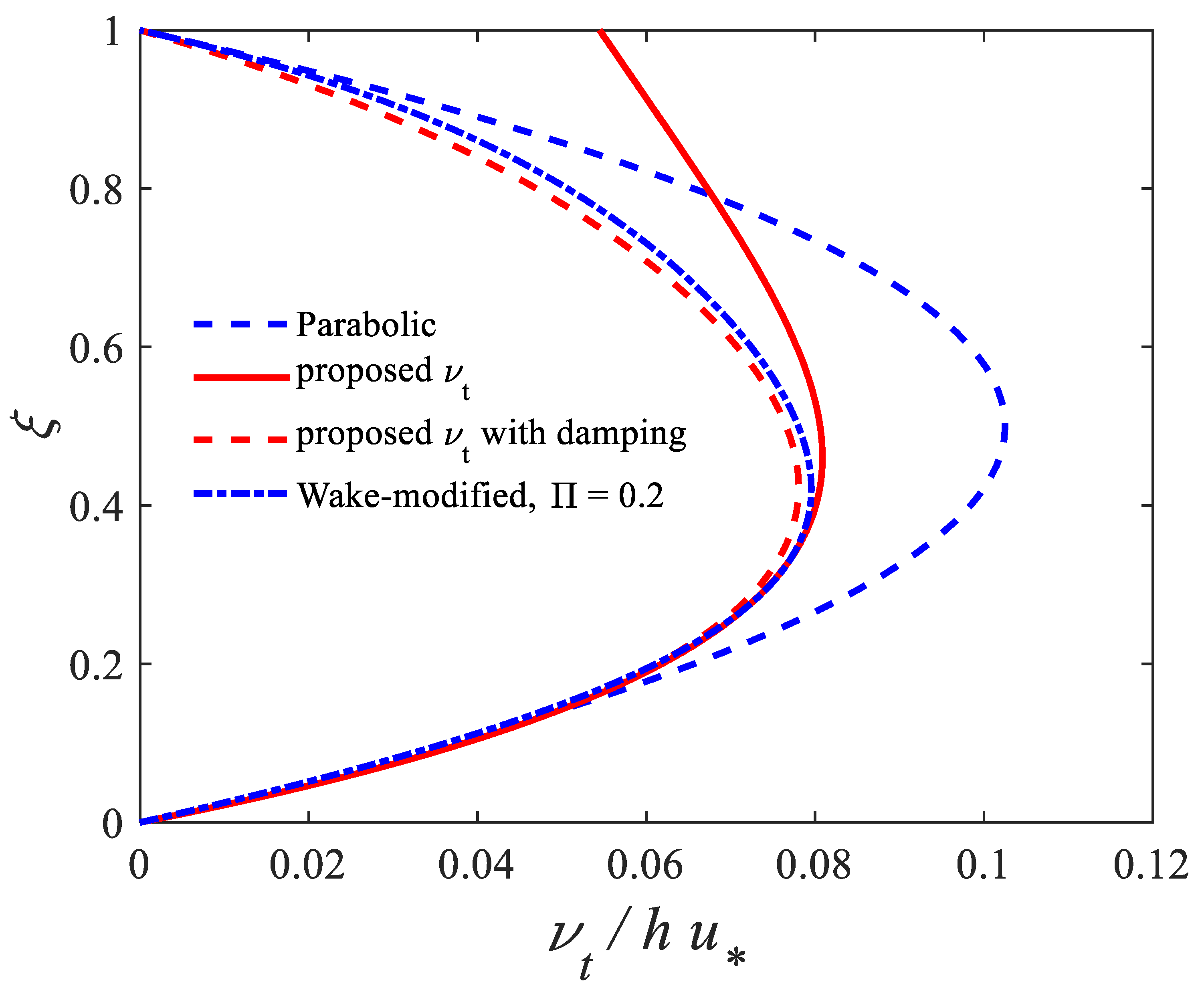
for large values of $R{e}_{*}$ ($R{e}_{*}$>2000), Equation (4) becomes $R{e}_{*}$-independent, and the two coefficients $C_{\mathsf{\alpha }}={\mathsf{\alpha }}_1\mathsf{\kappa }$ and $C_1$ reach asymptotic values equal, respectively, to $C_{\mathsf{\alpha }}=0.477$ and $C_1=2.17$. Equation (4) reverts therefore to the ${Re}_{*}$-independent form (5) with $C_{\mathsf{\alpha }}=0.477$ and $C_1=2.17$ [34]. With an additional correction to account for the damping effect of the turbulence near the free surface, we use a damping function in order to decrease the turbulent viscosity near the free surface as

$${\nu }_t\left(\xi \right)=C_{\mathsf{\alpha }} u_{*}y{e}^{-C_1\xi }\left(1-e^{-B_f\left(1-\xi \right)}\right)$$

(6)

Figure 1 shows the eddy viscosity profiles given by Equations (5) (red solid line) and (6) (red dashed line) and the comparisons with the parabolic and wake-modified profiles. The profile of Equation (6) is similar to the wake-modified profile with the value Π = 2 used for the open-channel flows [35]. Equations (5) and (6) provide identical results for $\xi <0.3$ and therefore Equation (5) could be used for the sediment transport modeling.

3.2. Turbulent Schmidt Number

Different studies were conducted toward developing equations for the turbulent Schmidt number or $\beta$-factor for both the steady and oscillatory flows [22,25,26,27,36,37,38,39].

The finite mixing length model allows writing the sediment diffusivity as [19]

$${\epsilon }_s=w_m{l}_m\left[1+\frac{l_m^2}{24}\frac{\frac{d^{3}C}{d{y}^3}}{\frac{dC}{dy}}+\dots \right],$$

(7)

with an eddy viscosity given by ${\nu }_t=w_m{l}_m$ (a product of mixing length $l_m$ and mixing velocity $w_m$) and the assumption of an exponential decreasing concentration profile given by $c=c_b{e}^{-A\xi }$, Equations (3) and (7) provide an equation for $\beta \left(y\right)$ as [38]

$$\beta \left(y\right)=1+\frac{l_m{}^2}{24} A^2,$$

(8)

with a linear mixing length equation ($l_m=\lambda y$) and $\lambda$ = 1 [19], (8) reverts to

$$\beta \left(y\right)=1+\frac{A^2}{24} y^2,$$

(9)

Equation (9) is similar to that proposed in [22]. Another empirical equation for $\beta \left(y\right)$ was proposed as [22]

$$\beta \left(y\right)={\beta }_b{f}_b\left(y\right)={\beta }_b{e}^{C_b\xi },$$

(10)

where ${\beta }_b$ and $C_b$ are the two coefficients. The Equation (10) allows to the sediment diffusivity ${\epsilon }_s$ to keep the same shape as eddy viscosity ${\nu }_t$ (5) by changing the value of the coefficient $C_1$ thanks to $C_b$ as

$${\epsilon }_s=\beta {\nu }_t={\beta }_b{e}^{C_b\xi }{C}_{\mathsf{\alpha }} u_{*}y{e}^{-C_1\xi }=C_{\mathsf{\alpha }\beta } u_{*}y{e}^{-C_{1\beta }\xi },$$

where $C_{\mathsf{\alpha }\beta }={\beta }_b{C}_{\mathsf{\alpha }}$ and $C_{1\beta }=C_1-C_b$. The depth-averaged $\beta$-factor is obtained by integrating $\beta \left(y\right)$ over the water column as

$${\beta }_{ave}=\frac{1}{h}{{\displaystyle \int }}_0^h\beta \left(y\right)dy={{\displaystyle \int }}_0^1\beta \left(\xi \right)d\xi ,$$

(11)

Using Equation (9), the integration of (11) gives the depth-averaged $\beta$-factor as

$${\beta }_{ave}=1+\frac{A^2}{72},$$

(12)

The coefficient $A$ is given by [37]

$$A=5.853+6.401\frac{\omega }{u_{*}},$$

(13)

By using Equation (13) in Equation (12), ${\beta }_{ave}$ becomes

$${\beta }_{ave}=1.47+1.03\left(\frac{\omega }{u_{*}}\right)+0.57{\left(\frac{\omega }{u_{*}}\right)}^2,$$

while by using a linear function given by $A=11\frac{\omega }{u_{*}}$ in Equation (12), ${\beta }_{ave}$ becomes [38]

$${\beta }_{ave}=1+1.68 {\left(\frac{\omega }{u_{*}}\right)}^2$$

(14)

Equation (14) is similar to a former empirical equation ${\beta }_{ave}=1+2 {\left(\frac{\omega }{u_{*}}\right)}^2$ [25].

4. Suspended Sediments in Steady Uniform Open-Channel Flows

4.1. The Kinetic Model and the Classical Advection–Diffusion Equation

The kinetic model was used for the suspended sediment in open-channel flows [17]. The concentration profiles from the kinetic model were compared to the experimental data [16] for the coarse sediments with the particle diameter $d_p=1.3 \mathrm{mm}$ (Table 1). The predicted concentration profiles for the coarse sediments obtained from the ADE, fail to predict the measured concentrations while the kinetic model shows good agreement. These results were related [17] to a weakness in the classical ADE, where the authors explained these profiles by the effects of lift the force and sediment stress gradient, which are significant for $\xi =y/h<0.1$.

However, it is possible to write the kinetic model of Equation (2) in two different forms related to the ADE (1).

In the first form, (2) is written as

$${\epsilon }_s\frac{dc}{dy}+{\omega }_s^{*}c=0,$$

(15)

where

$${\omega }_s^{*}=\left(1-\frac{{\tau }_p\left(F_L+F_{syns}\right)}{{\omega }_s}\right){\omega }_s$$

Equation (15) shows the effect of the kinetic model (2) as a hindered settling with a modified or “apparent” settling velocity ${\omega }_s^{*}$. Note that, for ${\tau }_p\left(F_L+F_{syns}\right)\ll {\omega }_s$, (15) reverts to (1).

In the second form, (2) is written as

$${\epsilon }_s^{*}\frac{dc}{dy}+{\omega }_{s}c=0,$$

(16)

where

$${\epsilon }_s^{*}=\frac{1}{1-\frac{{\tau }_p\left(F_L+F_{syns}\right)}{{\omega }_s}}{\epsilon }_s$$

Equation (16) shows the effect of the kinetic model (2) as a modified or “apparent” sediment diffusivity ${\epsilon }_s^{*}$. The same condition ${\tau }_p\left(F_L+F_{syns}\right)\ll {\omega }_s$ allows (15) to revert to (1). Since the kinetic model (2) is related to the ADE (1), this later is able to provide the same results as (2) with an adequate description of the “apparent” settling velocity or “apparent” sediment diffusivity.

4.2. Concentration Profile with the Advection–Diffusion Equation

It is possible to write Equation (1) as

$$\frac{dc}{dy}=-\frac{1}{R}c$$

(17)

where $R={\epsilon }_s/{\omega }_s$ is the ratio between the sediment diffusivity and the settling velocity. Note that both different forms given above by Equations (15) and (16) revert to Equation (17) with $R$ given, respectively, by $R={\epsilon }_s/{\omega }_s^{*}$ or $R={\epsilon }_s^{*}/{\omega }_s$.

Table 1. Flow conditions of experiments of Einstein and Chien [16].

Run Number	$\mathbf{h}\left(\mathbf{c}\mathbf{m}\right)$	${\mathit{d}}_{\mathit{p}}\left(\mathbf{m}\mathbf{m}\right)$	${\mathit{u}}_{*}\left(\mathbf{c}\mathbf{m}/\mathbf{s}\right)$	${\mathit{\rho }}_{\mathit{s}}/{\mathit{\rho }}_{\mathit{f}}$
S2	12.0	1.3	12.85	2.65
S3	11.7	1.3	13.26	2.65
S4	11.5	1.3	14.28	2.65

Table 1. Flow conditions of experiments of Einstein and Chien [16].

Run Number	$\mathbf{h}\left(\mathbf{c}\mathbf{m}\right)$	${\mathit{d}}_{\mathit{p}}\left(\mathbf{m}\mathbf{m}\right)$	${\mathit{u}}_{*}\left(\mathbf{c}\mathbf{m}/\mathbf{s}\right)$	${\mathit{\rho }}_{\mathit{s}}/{\mathit{\rho }}_{\mathit{f}}$
S2	12.0	1.3	12.85	2.65
S3	11.7	1.3	13.26	2.65
S4	11.5	1.3	14.28	2.65

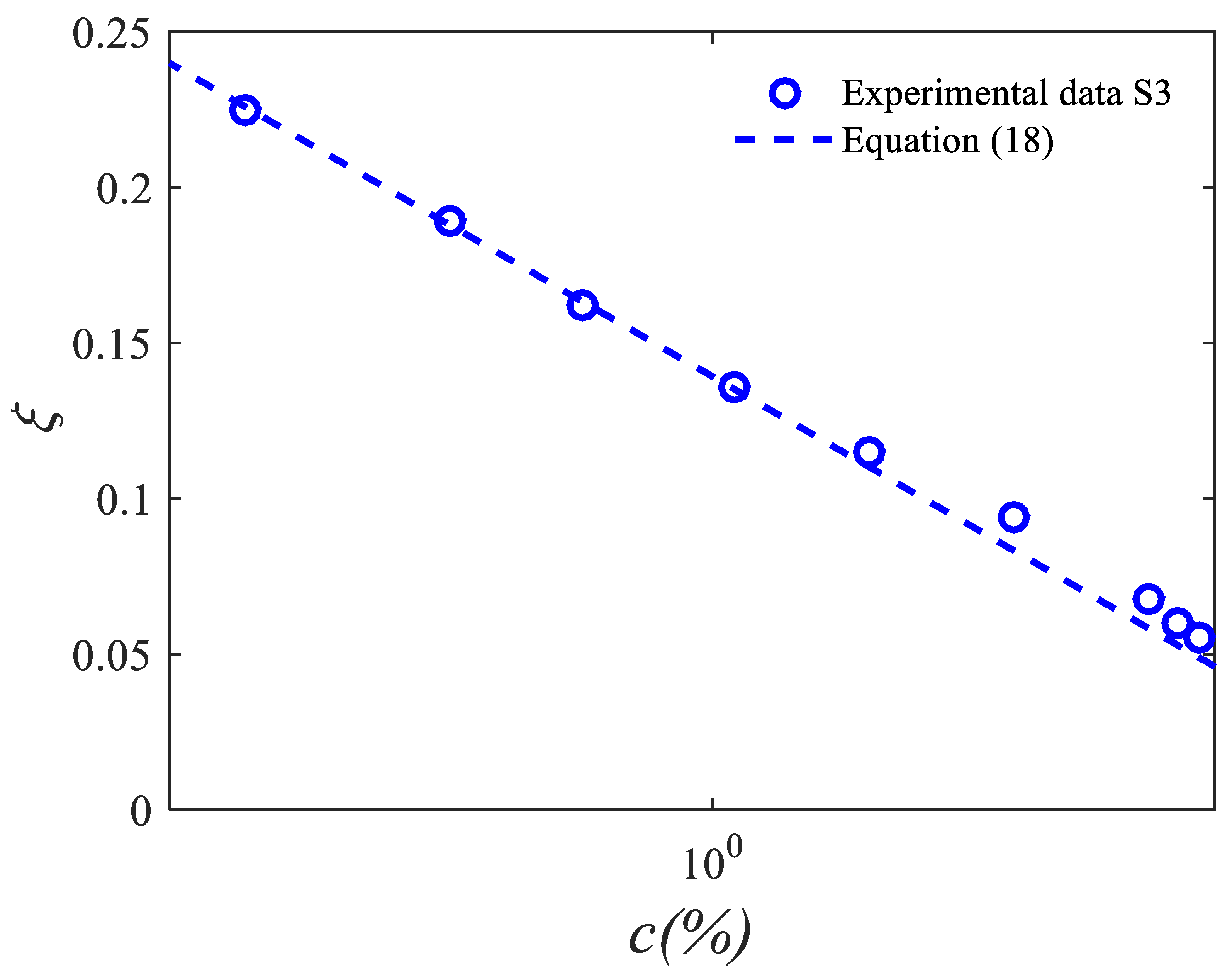
By assuming that this ratio becomes a constant equal to a concentration length scale $R=L_c$, the integration of Equation (1) gives the well-known exponential decreasing concentration profile

$$c\left(y\right)=c_a exp\left(-\frac{y-a}{L_c}\right),$$

(18)

where $c_a=c\left(y=a\right)$ and $L_c$ is the concentration profile length scale. Equation (18) allows analysis of the experimental data. In the semi-log plot, Equation (18) is represented by a straight line (Figure 2) which fits the experimental data for $\xi >0.1$. However, for $\xi <0.1$, the experimental data deviate from the straight line. This seems to be associated to a decrease in the particles’ settling velocity for high concentrations, in particular for the case of coarse sediments (i.e., hindered settling velocity).

4.3. Hindered Settling Velocity

For the prediction of the suspended sediment concentration profiles, the settling velocity of the sediment particles in the ADE was often taken as a constant. However, in sediment-laden flows, the settling velocity is reduced due to the presence of particles and high concentrations near the bed/bottom (i.e., hindered settling velocity). Different studies have been undertaken to predict the distribution of the sediment concentration incorporating this effect [22,37,38]. In the present study, we write an $y$-dependent settling velocity as [22]

$${\omega }_s\left(y\right)={\omega }_{s0} f_s\left(y\right),$$

(19)

where ${\omega }_{s0}$ is the terminal settling velocity of a particle alone in an infinite fluid and $f_s\left(y\right)$ is a function that is equal to 1 far from the bed where concentrations are very small and decrease near the bed for high concentrations. Since $f_s\left(y\right)\approx 1$ in the outer region, we can write $L_c\approx \left(\beta {\nu }_t\right)/{\omega }_{s0}$ with the product $\beta {\nu }_t$ which seems to be $y$-independent over a given elevation. However, we need to consider that $f_s\left(y\right)\ne 1$ in the inner region where we write $R\left(y\right)=L_c/f_s\left(y\right)$. Experiments have demonstrated that the particle settling velocities are lower at higher concentrations. This behavior is given by the well-known semi-empirical equation of Richardson and Zaki [28]

$${\omega }_s={\omega }_{s0}{\left(1-c\right)}^n,$$

(20)

where $n$ is an empirically determined exponent dependent on the particle Reynolds number $R_t$ at ${\omega }_{s0}$ and is constant for a particular particle. This exponent was determined experimentally as between 4.65 and 2.4 for increasing $R_t$.

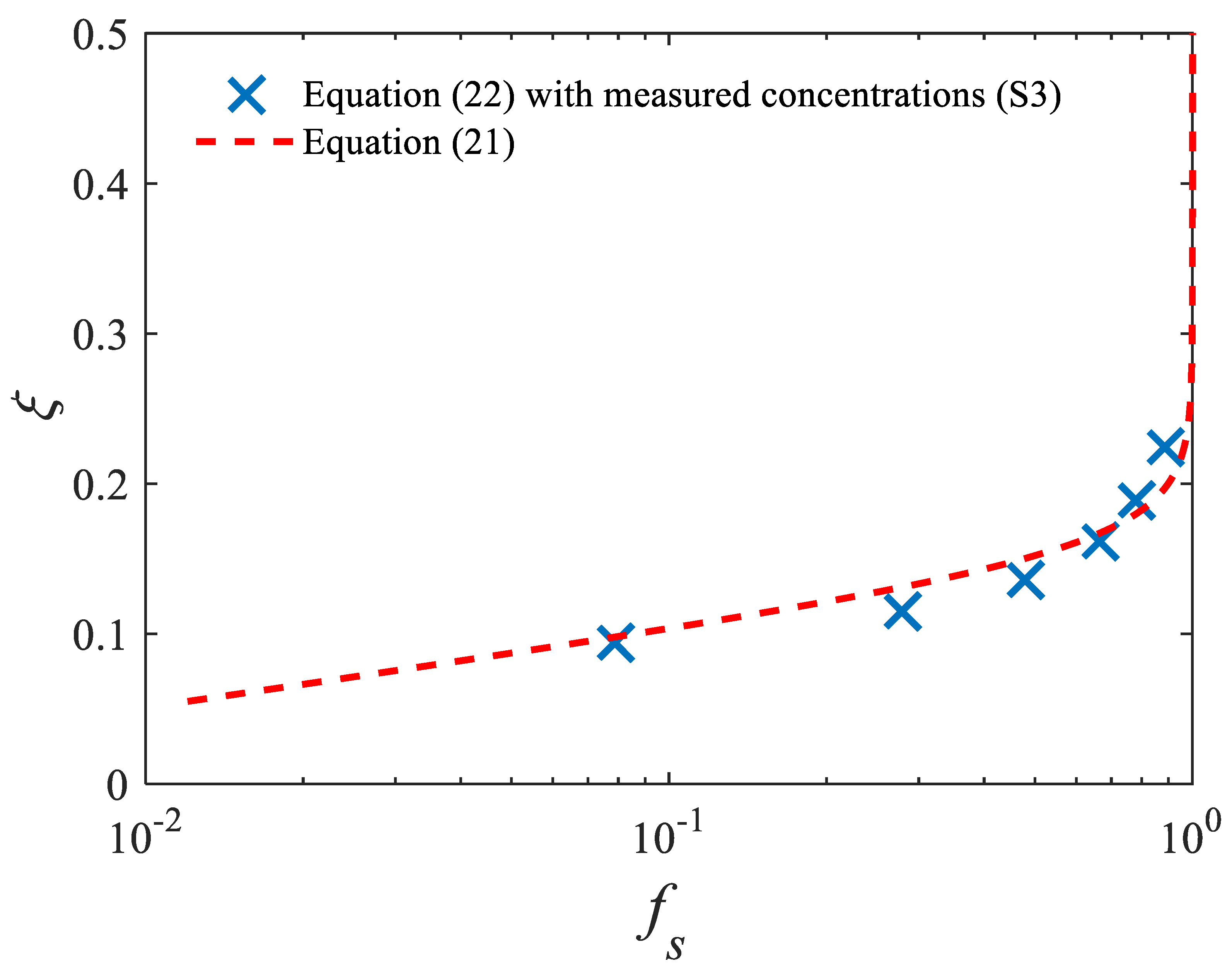
In order to verify that the observed near-bed upward convex concentration profile for coarse sediments is related to the decreasing settling velocity, the following empirical function for $f_s\left(y\right)$ was proposed [22]

$$f_s\left(y\right)=\frac{{\omega }_s\left(y\right)}{{\omega }_{s0}}=\frac{1}{1+{\alpha }_{s}exp\left(-y/h_s\right)}$$

(21)

where $h_s$ and ${\alpha }_s$ are two parameters that depend on the concentrations and the sediment grain size. Equation (21) is validated (Figure 3) by the experimental data of $f_s\left(y\right)$ obtained from Equation (20) and the measured $c$-values as

$$f_s{}_{exp}={\left(1-c_{exp}\right)}^n$$

(22)

4.4. Results

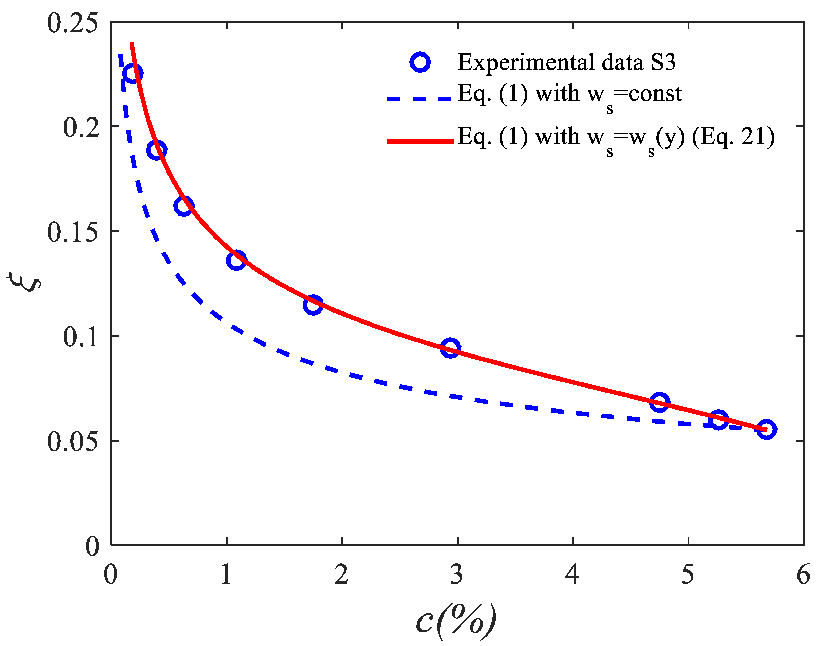
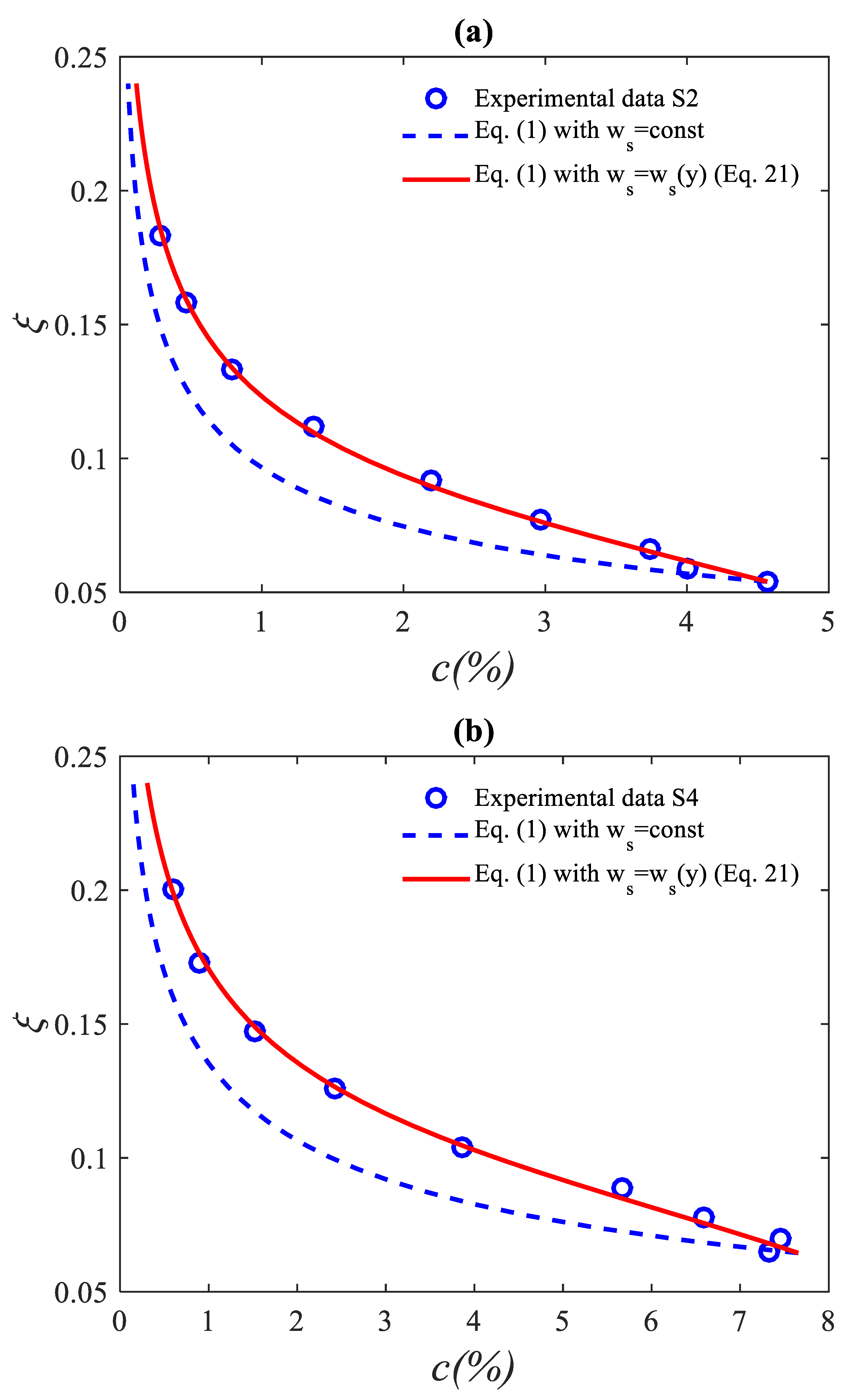
Figure 4 and Figure 5 show the comparison between the predicted concentration profiles and the experimental data for the coarse sediments (Table 1) [16]. In Figure 4, the measurements (symbols) show, in the Cartesian coordinates, the main upward concave concentration profile for $\xi >0.1$ which corresponds to the straight line, in the semi-log plot, given by Equation (18) in Figure 2. The concentration profiles are obtained from ADE (1). In Figure 4, the sediment diffusivity ${\epsilon }_s$ is given by (3), ${\nu }_t\left(y\right)$ from (5) and $\beta \left(y\right)$ from (9) and (13). The blue dashed line is for a constant ${\omega }_s={\omega }_{s0}$ while the red solid line corresponds to ${\omega }_s\left(y\right)={\omega }_{s0} f_s\left(y\right)$ given by (21). Concentration profiles show that $\beta$ is very close to 1. In order to study the effect of hindering settling, the concentration profiles (Figure 5) are obtained from ADE (1) with ${\epsilon }_s={\nu }_t$ given by (5) ($\beta =1)$. For the settling velocity, constant ${\omega }_s={\omega }_{s0}$ (blue dashed lines) and ${\omega }_s\left(y\right)={\omega }_{s0} f_s\left(y\right)$ given by (21) (red solid lines). The predicted concentration profiles obtained by the ADE with the hindering settling (red solid lines) show good agreement with the experimental data (symbols) for the coarse sediments (Table 1).

Figure 4 and Figure 5 confirm the ability of the ADE to predict the overall measured concentrations with a suitable description of the vertical distribution of the settling velocity ${\omega }_s$ over the flow depth (red solid lines).

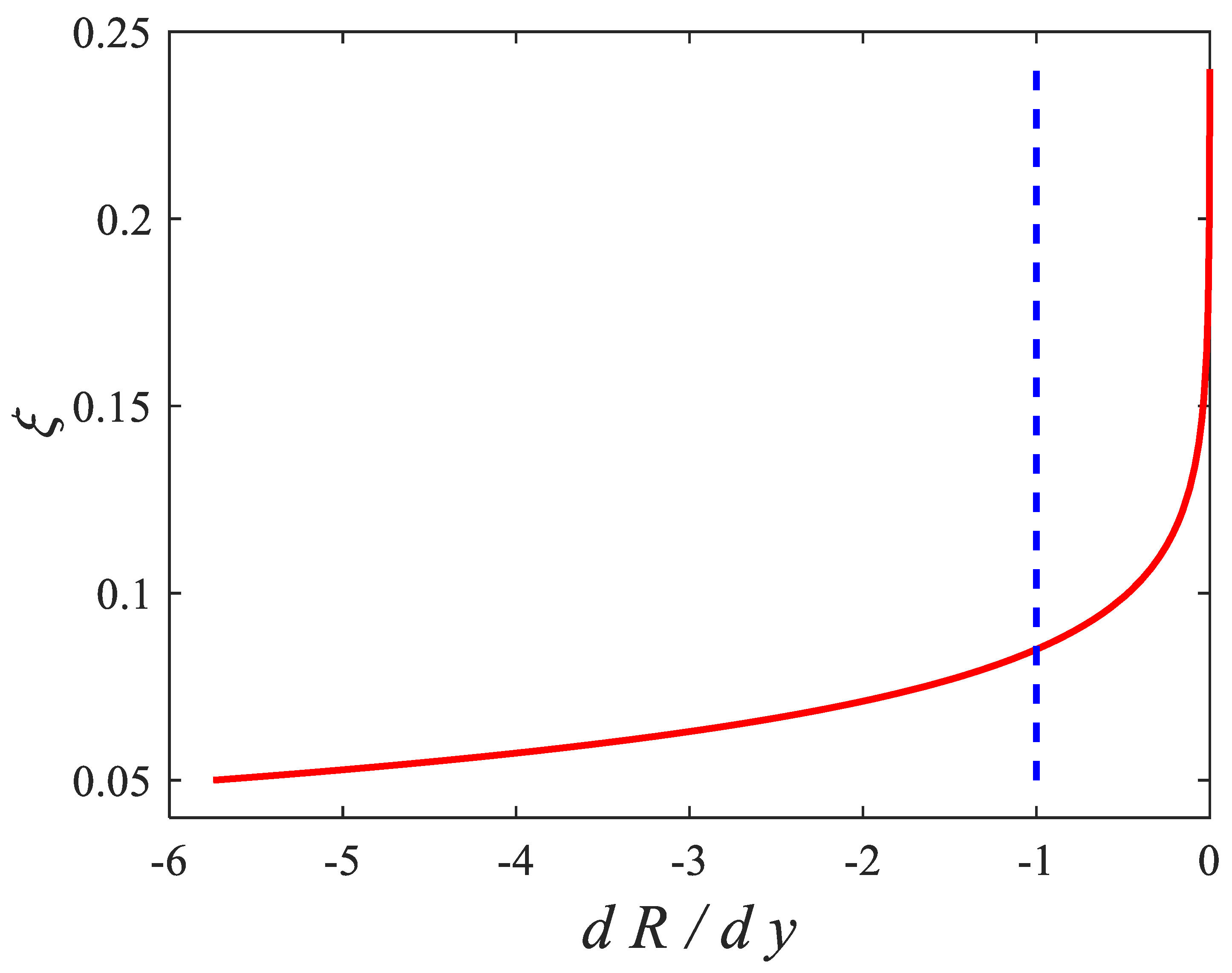
4.5. First Criterion for Concentration Profiles Shape in Cartesain Coordiantes

Derivative of Equation (1) (by using Equation (18)) allows writing

$$\frac{d^{2}c}{d{y}^2}=\frac{c}{R^2}\left(\frac{dR}{dy}+1\right)$$

(23)

The upward concavity/convexity of the concentration profiles is related to the sign of $\frac{d^{2}c}{d{y}^2}$ and therefore to the sign of $\frac{dR}{dy}+1$ since $\frac{c}{R^2}$ is always >0 ($\frac{d^{2}c}{d{y}^2}$ and $\frac{dR}{dy}+1$ have the same sign). Therefore, the upward concave concentration profiles correspond to $\frac{dR}{dy}>-1$ while the upward convex concentration profiles correspond to $\frac{dR}{dy}<-1$.

The classical ADE is therefore able to predict the near-bed upward convex concentration profile if the derivative of the ratio between the sediment diffusivity and the settling velocity is lower than −1 (Figure 6).

Figure 5. Concentration profiles for coarse sediments. Curves from numerical resolution of ADE (1) with ${\epsilon }_s={\nu }_t$ (5) $C_{\mathsf{\alpha }}=0.477$ and $C_1=2.17$; dashed lines: constant settling velocity ${\omega }_s={\omega }_{s0}=0.1411\mathrm{m}/\mathrm{s}$; solid lines: ${\omega }_s\left(y\right)={\omega }_{s0} f_s\left(y\right)$ (21); symbols: experimental data (a) S2 ${\alpha }_s=32$, $h_s=0.019$; (b) S4 ${\alpha }_s=70$, $h_s=0.019$.

Figure 5. Concentration profiles for coarse sediments. Curves from numerical resolution of ADE (1) with ${\epsilon }_s={\nu }_t$ (5) $C_{\mathsf{\alpha }}=0.477$ and $C_1=2.17$; dashed lines: constant settling velocity ${\omega }_s={\omega }_{s0}=0.1411\mathrm{m}/\mathrm{s}$; solid lines: ${\omega }_s\left(y\right)={\omega }_{s0} f_s\left(y\right)$ (21); symbols: experimental data (a) S2 ${\alpha }_s=32$, $h_s=0.019$; (b) S4 ${\alpha }_s=70$, $h_s=0.019$.

5. Suspended Sediments in Oscillatory Flows over Sand Ripples

5.1. Convection–Diffusion Equation with Upward Convection Term

For suspended sediments in oscillatory flows over sand ripples, in addition to the “diffusive mechanism” related to the sediment diffusivity ${\epsilon }_s$, another process is a coherent phenomenon related to vortex formation and shedding at the flow reversal above the ripples, which is “a convective mechanism” [4].

The ADE (1) was adapted by adding an additional term related to the convective mechanism $F_{conv}$. The convection–diffusion model for the time-averaged concentrations (over the wave period) is given by [4]

$${\epsilon }_s\frac{dc}{dy}+{\omega }_{s}c+F_{conv}=0,$$

(24)

the respective terms in (24) represent: upward diffusion, which represents a pure disorganized ‘‘diffusive” process and downward settling and upward convection $F_{conv}$ which describes the coherent convective sediment entrainment process.

We wrote Equation (24) in the form of Equation (16) [40] with a modified or apparent sediment diffusivity ${\epsilon }_s^{*}$ instead of ${\epsilon }_s$, given by

$${\epsilon }_s^{*}=\frac{1}{1+\frac{F_{conv}}{{\omega }_{s}c}}{\epsilon }_s=1+\frac{F_{conv}}{{\epsilon }_s\frac{dc}{dy}}{\epsilon }_s=\alpha {\epsilon }_s$$

(25)

where the parameter $\alpha$ is related to the convective sediment entrainment process associated with the process of vortex shedding above the ripples. This parameter $\alpha$ was interpreted by two different expressions (Equation (25)). In the first, α depends on the relative importance of the upward convection $F_{conv}$ related to the coherent vortex shedding and downward settling of the sediments ${\omega }_{s}c$. In the second, α depends on the relative importance of terms $F_{conv}$ and $F_{diff}={\epsilon }_{s}dc/dy$ which are related, respectively, to the coherent vortex shedding and random turbulence. An empirical function for $\mathsf{\alpha }$ was proposed by [40]

$$\alpha =1+D e^{-\frac{y}{h_s}}$$

(26)

where $D$ and $h_s$ are two parameters. The eddy viscosity for the steady flows given by Equation (6) was generalized to the oscillatory flows [40,41,42,43,44,45].

From Equations (5), (10) and (26) we wrote ${\epsilon }_s^{*}$ as [40]

$$\frac{{\epsilon }_s^{*}}{U_0{k}_s}=A_s\frac{y}{k_s}{e}^{-\frac{y}{B_s}} \left(1+D e^{-\frac{y}{h_s}}\right)$$

(27)

The vertical distribution of the sediment diffusivity given by Equation (27) was confirmed by the experimental data and it is similar to a former empirical distribution which is constant then linear. The near-bed constant region is due to the coherent vortex formation and shedding related to the flow separation on the lee side of the steep ripple crest. In the following layer, the linearly increasing profile for the sediment diffusivity is related to the random turbulent processes and gradient diffusion. Indeed, the vortices lose their coherence in this layer [46,47,48,49,50].

5.2. Second Criterion for Concentration Profiles Shape in Semi-Log Plots

The concentration profiles were interpreted by a relation between the second derivative of the logarithm of the concentration and the derivative of the product between the sediment diffusivity and α. It is possible to write from Equation (16) [22]

$$\frac{d^{2}ln\left(c\right)}{d{y}^2}=\frac{{\omega }_s}{{\epsilon }_s^{*}{}^2}\frac{d{\epsilon }_s^{*}}{dy}$$

(28)

Equation (28) provides, in the semi-log plots, a link between the upward concavity/convexity of the concentration profiles and the increasing/decreasing in ${\epsilon }_s^{*}$. Increasing ${\epsilon }_s^{*}$ allows the upward concave concentration profile, while decreasing ${\epsilon }_s^{*}$ allows an upward convex concentration profile.

6. Conclusions

This study is related to the near-bed/bottom concentration profiles for coarse sediments in environmental flows.

The findings of the present study can be summarized in the following conclusions:

-

In this study, we provided simple and accurate tools for the sediment diffusivity through analytical formulations for both the eddy viscosity and β-factor/function (i.e., the inverse of the turbulent Schmidt number).

-

For steady open-channel flows, two models were investigated, namely, the ADE and the kinetic model.

-

Our study shows that the kinetic model reverts to the classical ADE with a modified or “apparent” settling velocity.

-

Results for the concentration profiles, with a hindered settling function, show good agreement for the open-channel flows.

-

An interpretation of the concentration profiles is provided.

-

For steady open-channel flows: the concentration profiles shape, in the Cartesian coordinates, depends on the vertical distribution of the derivative of the ratio R between the sediment diffusivity and the settling velocity of the sediments ($dR/dy$): $dR/dy>-1$ for the upward concave concentration profile while $dR/dy<-1$ for the near-bed upward convex profile.

-

For oscillatory flows over sand ripples, the convection–diffusion equation was considered. As for the kinetic model, the convection–diffusion equation reverts to the classical ADE but with an “apparent” sediment diffusivity instead of the “apparent” settling velocity.

-

A generalization was proposed for the interpretation of the concentration profiles for fine and coarse sand in oscillatory flows over sand ripples. A relation between the second derivative of the logarithm of the concentration and the derivative of the apparent sediment diffusivity allows interpretation of the concentration profiles in the semi-log plots. This equation provides a link, in the semi-log plots, between the upward concavity/convexity of the concentration profiles and the increasing/decreasing in the apparent sediment diffusivity. Increasing the apparent sediment diffusivity allows an upward concave concentration profile, while decreasing the apparent sediment diffusivity allows an upward convex concentration profile.

References

- Vanoni, V.A. Transportation of Suspended Sediment by Water; ASCE: Reston, VA, USA, 1946; Volume 111, pp. 67–133. [Google Scholar]
- Yalin, M.S. Mechanics of Sediment Transport; Pergamon Press: Oxford, UK, 1972. [Google Scholar]
- Fredsoe, J.; Deigaard, R. Mechanics of Coastal Sediment Transport; World Scientific Publishing: Singapore, 1992; 369p. [Google Scholar]
- Nielsen, P. Coastal Bottom Boundary Layers and Sediment Transport; World Scientific Publishing: Singapore, 1992; 324p. [Google Scholar]
- Seminara, G.; Blondeaux, P. River, Coastal and Estuarine Morphodynamics; Springer: Berlin/Heidelberg, Germany, 2001. [Google Scholar]
- Guo, J.; Wood, W.L. Fine Suspended Sediment Transport Rates. J. Hydraul. Eng. ASCE 1995, 121, 919–922. [Google Scholar] [CrossRef]
- Tsai, C.W.; Hung, S.Y. Modeling Suspended Sediment Transport Under Influence of Turbulence Ejection and Sweep Events. Water Resour. Res. 2019, 55, 5379–5393. [Google Scholar] [CrossRef]
- Ghoshal, K.; Jain, P.; Absi, R. Nonlinear Partial Differential Equation for Unsteady Vertical Distribution of Suspended Sediments in Open Channel Flows: Effects of Hindered Settling and Concentration-Dependent Mixing Length. J. Eng. Mech. ASCE 2022, 148, 04021123. [Google Scholar] [CrossRef]
- Gaudio, R. Turbulence and Flow–Sediment Interactions in Open-Channel Flows. Water 2020, 12, 3169. [Google Scholar] [CrossRef]
- Lai, Y.G.; Wu, K.A. Three-Dimensional Flow and Sediment Transport Model for Free-Surface Open Channel Flows on Unstructured Flexible Meshes. Fluids 2019, 4, 18. [Google Scholar] [CrossRef] [Green Version]
- Hu, L.; Dong, Z.; Peng, C.; Wang, L.-P. Direct Numerical Simulation of Sediment Transport in Turbulent Open Channel Flow Using the Lattice Boltzmann Method. Fluids 2021, 6, 217. [Google Scholar] [CrossRef]
- Faraci, C.; Scandura, P.; Petrotta, C.; Foti, E. Wave-Induced Oscillatory Flow over a Sloping Rippled Bed. Water 2019, 11, 1618. [Google Scholar] [CrossRef] [Green Version]
- Gusarov, A.V.; Sharifullin, A.G.; Komissarov, M.A. Contemporary Long-Term Trends in Water Discharge, Suspended Sediment Load, and Erosion Intensity in River Basins of the North Caucasus Region, SW Russia. Hydrology 2021, 8, 28. [Google Scholar] [CrossRef]
- Jain, P.; Kundu, S.; Ghoshal, K.; Absi, R. Direct Derivation of Streamwise Velocity from RANS Equation in an Unsteady Nonuniform Open-Channel Flow. J. Eng. Mech. ASCE 2022, 148, 06022002. [Google Scholar] [CrossRef]
- Sen, S.; Kundu, S.; Absi, R.; Ghoshal, K. A model for coupled fluid velocity and suspended sediment concentration in an unsteady stratified turbulent flow through an open channel. J. Eng. Mech. ASCE 2023, 149, 04022088. [Google Scholar] [CrossRef]
- Einstein, H.A.; Chien, N. Effects of Heavy Sediment Concentration Near the Bed on Velocity and Sediment Distribution; M.R.D. Sediment Series, Rep. No. 8; University of California: Berkeley, CA, USA, 1955. [Google Scholar]
- Fu, X.; Wang, G.; Shao, X. Vertical dispersion of fine and coarse sediments in turbulent open-channel flows. J. Hydraul. Eng. ASCE 2005, 131, 877–888. [Google Scholar] [CrossRef]
- McFetridge, W.F.; Nielsen, P. Sediment Suspension by Non-Breaking Waves over Rippled Beds; Technical Report No. UFL/COEL-85/005; Coast Ocean Eng Dept, University of Florida: Gainesville, FL, USA, 1985. [Google Scholar]
- Nielsen, P.; Teakle, I.A.L. Turbulent diffusion of momentum and suspended particles: A finite-mixing-length-theory. Phys. Fluids 2004, 16, 2342–2348. [Google Scholar] [CrossRef]
- Absi, R. Comment on Turbulent diffusion of momentum and suspended particles: A finite-mixing-length theory. Phys. Fluids 2005, 17, 079101. [Google Scholar] [CrossRef] [Green Version]
- Absi, R. Modeling turbulent mixing and sand distribution in the bottom boundary layer. In Proceedings of the 5th International Conference on Coastal Dynamics 2005—State of the Practice, Barcelona, Spain, 4–8 April 2005; Sanchez-Arcilla, A., Ed.; ASCE: Reston, VA, USA, 2005. [Google Scholar]
- Absi, R. Concentration profiles for fine and coarse sediments suspended by waves over ripples: An analytical study with the 1-DV gradient diffusion model. Adv. Water Resour. 2010, 33, 411–418. [Google Scholar] [CrossRef] [Green Version]
- Rouse, H. Modern conceptions of the mechanics of fluid turbulence. Trans. Am. Soc. Civ. Eng. 1937, 102, 463–543. [Google Scholar] [CrossRef]
- Umeyama, M. Velocity and concentration fields in uniform flow with coarse sands. J. Hydraul. Eng. ASCE 1999, 125, 653–656. [Google Scholar] [CrossRef]
- Van Rijn, L.C. Sediment Transport, Part II: Suspended Load Transport. J. Hydraul. Eng. ASCE 1984, 110, 1613–1641. [Google Scholar] [CrossRef]
- Graf, W.H.; Cellino, M. Suspension flows in open channels: Experimental study. J. Hydraul. Res. 2002, 40, 435–447. [Google Scholar] [CrossRef]
- Kaushal, D.R. Discussion of Vertical dispersion of fine and coarse sediments in turbulent open-channel flows. J. Hydraul. Eng. ASCE 2007, 133, 1292–1294. [Google Scholar] [CrossRef]
- Richardson, J.F.; Zaki, W.N. Sedimentation and fluidisation: Part 1. Trans. Inst. Chem. Eng. 1954, 32, 35–53. [Google Scholar] [CrossRef]
- Absi, R. Time-dependent eddy viscosity models for wave boundary layers. In Proceedings of the 27th International Conference on Coastal Engineering, Sydney, Australia, 16–21 July 2000; Edge, B.L., Ed.; ASCE Press: Reston, VA, USA, 2001; Volume 2, pp. 1268–1281. [Google Scholar]
- Absi, R. Analytical solutions for the modeled k-equation. ASME J. Appl. Mech. 2008, 75, 044501. [Google Scholar] [CrossRef]
- Absi, R. A simple eddy viscosity formulation for turbulent boundary layers near smooth walls. C. R. Mec. 2009, 337, 158–165. [Google Scholar] [CrossRef] [Green Version]
- Absi, R. Eddy viscosity and velocity profiles in fully-developed turbulent channel flows. Fluid Dyn. 2019, 54, 137–147. [Google Scholar] [CrossRef]
- Absi, R. Analytical eddy viscosity model for velocity profiles in the outer part of closed- and open-channel flows. Fluid Dyn. 2021, 56, 577–586. [Google Scholar] [CrossRef]
- Absi, R. Reinvestigating the parabolic-shaped eddy viscosity profile for free surface flows. Hydrology 2021, 8, 126. [Google Scholar] [CrossRef]
- Nezu, I.; Nakagawa, H. Turbulence in Open-Channel Flows; A.A. Balkema: Rotterdam, The Netherlands, 1993. [Google Scholar]
- Absi, R.; Marchandon, S.; Lavarde, M. Turbulent diffusion of suspended particles: Analysis of the turbulent Schmidt number. Defect Diffus. Forum 2011, 312–315, 794–799. [Google Scholar] [CrossRef]
- Jain, P.; Kumbhakar, M.; Ghoshal, K. A mathematical model on depth-averaged β-factor in open-channel turbulent fow. Environ. Earth Sci. 2018, 77, 253. [Google Scholar] [CrossRef]
- Absi, R. Rebuttal on A mathematical model on depth-averaged β-factor in open-channel turbulent flow. Environ. Earth Sci. 2020, 79, 113. [Google Scholar] [CrossRef]
- Gualtieri, C.; Angeloudis, A.; Bombardelli, F.; Jha, S.; Stoesser, T. On the Values for the Turbulent Schmidt Number in Environmental Flows. Fluids 2017, 2, 17. [Google Scholar] [CrossRef] [Green Version]
- Absi, R.; Tanaka, H. Analytical eddy viscosity model for turbulent wave boundary layers: Application to suspended sediment concentrations over wave ripples. J. Mar. Sci. Eng. submitted.
- Absi, R. Calibration of Businger-Arya type of eddy viscosity model’s parameters. J. Waterw. Port Coast. Ocean Eng. ASCE 2000, 126, 108–109. [Google Scholar] [CrossRef]
- Absi, R. Wave boundary layer instability near flow reversal. In Proceedings of the 28th International Conference on Coastal Engineering 2002, Cardiff, UK, 7–12 July 2002; Smith, J.M., Ed.; World Scientific Publishing: Singapore, 2002; Volume 1, pp. 532–544, ISBN 981-238-238-0. [Google Scholar]
- Absi, R. Discussion of One-dimensional wave bottom boundary layer model comparison: Specific eddy viscosity and turbulence closure model. J. Waterw. Port Coast. Ocean Eng. ASCE 2006, 132, 139–141. [Google Scholar] [CrossRef]
- Absi, R. On the effect of sand grain size on turbulent mixing. In Proceedings of the International Conference on Coastal Engineering 2006, San Diego, CA, USA, 3–8 September 2006; Smith, J.M., Ed.; World Scientific Publishing: Singapore, 2006; pp. 3019–3029. [Google Scholar]
- Absi, R.; Tanaka, H.; Kerlidou, L.; André, A. Eddy viscosity profiles for wave boundary layers: Validation and calibration by a k-ω model. In Proceedings of the 33th International Conference on Coastal Engineering, Santander, Spain, 1–6 July 2012. [Google Scholar]
- Sheng, J.; Hay, A.E. Sediment eddy diffusivities in the nearshore zone, from multifrequency acoustic backscatter. Cont. Shelf Res. 1995, 15, 129–147. [Google Scholar] [CrossRef]
- Lee, T.H.; Hanes, D.M. Comparison of field observations of the vertical distribution of suspended sand and its prediction by models. J. Geophys. Res. 1996, 101, 3561–3572. [Google Scholar] [CrossRef]
- Van Rijn, L.C. United view of sediment transport by currents and waves II: Suspended transport. J. Hydraul. Eng. ASCE 2007, 133, 668–689. [Google Scholar] [CrossRef]
- Thorne, P.D.; Williams, J.J.; Davies, A.G. Suspended sediments under waves measured in a large-scale flume facility. J. Geophys. Res. 2002, 107, 3178. [Google Scholar] [CrossRef]
- Thorne, P.D.; Davies, A.G.; Bell, P.S. Observations and analysis of sediment diffusivity profiles over sandy rippled beds under waves. J. Geophys. Res. 2009, 114, C02023. [Google Scholar] [CrossRef]
Figure 1.
Eddy viscosity profiles; red solid line: eddy viscosity (5) with and ; red dashed line: eddy viscosity with free surface damping function (6) with ; blue dash-dotted line: log-wake-modified with Π = 0.2; blue dashed line: parabolic eddy viscosity.
Figure 2.
Concentration profile in semi-log plot, for coarse sediments.
Figure 3.
Vertical distribution of dimensionless settling velocity of sediments . Curve, Equation (21); symbols, experimental data from Equation (22) and measured concentrations (S3).
Figure 4.
Concentration profiles for coarse sediments (S3). Curves from numerical resolution of ADE (1) with (5) and ; from (9) and (13); dashed lines: constant settling velocity ; solid lines: (21) , ; symbols: experimental data.