Quantitative Analysis of Separated Impurities inside Filter Cakes with Phantom-Aided X-ray Tomography

Abstract

This study presents a new approach in the quantification of the deposited amount of impurity inside a filter cake made up of filter aid material. For this purpose, three-dimensional imaging by X-ray tomography is applied. Based on the X-ray attenuation properties, a model system consisting of kieselguhr as filter aid and barium sulphate as impurity is chosen. Due to the impurity particle size being smaller than the spatial resolution of the measuring setup, a calibration approach is necessary to gain insight into subvoxel information. A so-called phantom of similar material composition is prepared. The grey values are linearly correlated with the impurity volume fraction resulting in a calibration function, which facilitates the calculation of impurity volume fraction based on grey values measured inside the filter cake. First results are presented, showing that the approach delivers valid results for the chosen material system and reveals unexpected characteristics of the filter cake structure. Challenges in the context of the phantom approach and their influence on the obtained results are discussed.

1. Introduction

X-ray microcomputed tomography (micro-CT) is a three-dimensional imaging technique which allows nondestructive analysis of samples. Originally developed as a medical diagnostic tool with X-ray needle or fan beam geometry, further development towards powerful flat panel detectors enabled the construction of CT systems with cone beam geometry and, thus, a significant improvement in resolution and scanning speed [1]. In addition to the geometrical magnification, a setup with additional optics, a so-called X-ray microscope (XRM), allows a further increase in resolution by one order of magnitude. Nowadays, XRM systems which can achieve a resolution of a few µm have become a standard tool in the engineering sciences for the characterization of particle systems, for example to support the understanding of separation processes [2,3].

When penetrating the sample, X-rays are attenuated due to interactions of X-ray photons with the matter which is described by Beer–Lambert’s law:

$$\frac{I}{I_0}=\exp \left(-{{\displaystyle \int }}_0^L\mu \mathrm{d}s\right)$$

(1)

with $I_0$ and $I$ describing the intensity of X-rays before and after penetrating the sample, respectively. The linear attenuation coefficient of a specific material $\mu$ depends on the material density $\rho$ and is a function of the X-ray wavelength $\lambda$ and thus X-ray energy [1]. Although the attenuation is strongly influenced by the samples’ material properties, conventional computed tomography is not an element-specific analysis, as the attenuation is normally recorded through greyscale images. Then, during tomographic reconstruction, each smallest possible volume element, a so-called voxel, is assigned to a grey value, which is composed of the attenuation properties of all material phases contained in the respective volume. This summation of material properties inside a voxel is called partial volume effect (PVE) [4]. Mostly considered as an imaging artefact, the PVE can be used to obtain additional information: the grey value of voxels affected by the PVE can be assumed to be the linear mixture of the attenuation property of each contained phase, weighted by their respective volume fraction [5]. For polychromatic X-ray sources, this assumption can only be made if artefacts resulting from beam hardening are kept to a minimum [6]. Beam hardening occurs along the radial dimension of the sample, when low energy X-rays are attenuated more strongly in the center of the sample. Additionally, structural beam hardening results from highly attenuating material inside the sample. Both PVE and beam hardening lead to a change of grey value over the radial distance from the sample center and around highly attenuating structures [7].

To obtain quantitative information from a CT measurement, a segmentation is usually performed after post-processing of the reconstructed data. With each contained phase of the sample assigned to a specific grey value, the sample can be analyzed quantitatively. However, this method requires the structural feature of interest to be significantly larger than the voxel size in order to be able to be identified during image processing [8]. Although the PVE is present in the whole volume, it manifests itself visually mainly at interfaces between differently absorbing phases. As a result, these interfaces become blurred and can only be distinguished from neighboring phases if there is a minimum lateral distance of two to four voxels [6,9]. Thus, voxel size is an insufficient parameter when talking about resolution. Instead, spatial resolution as the minimum distance between to features that can be detected as individuals should be considered. For the used setup, a factor of five is assumed as the correlation between voxel and spatial resolution. The achievable voxel resolution—and thus the field of view (FOV)—is limited by the dimension of the sample unless the setup permits scanning within the sample [10]. Note that with larger features, and thus a larger FOV, the resolution decreases because both are linked via a fixed number of detector pixels [11]. Therefore, performing an adequate segmentation for a quantitative analysis will not be feasible if the particles of interest are smaller than the spatial resolution [12].

In spite of this challenge, there are other methods of performing quantitative analyses based on tomographic greyscale information. One of these approaches uses a calibration sample also known as a phantom. The method was originally developed in the field of medical imaging and aims at creating an object with precisely known properties that behaves as similarly as possible to the real object when imaged. Initially, the term “phantom” would refer to an object mimicking a part of the human body [13]. Medical phantoms are used to determine bone mineral content [14] or bone density [15], to evaluate electron density/proton stopping power for proton radiation therapy [16], to distinguish tissue types in breast tumor diagnosis [17], or to quantify the accumulation of drug particles in organs [18]. As of today, a phantom is any calibration sample with known defined material properties that is used to calibrate a grey value histogram to establish a clear link between the material property and a certain grey value. In most cases, the use of calibration samples serves the determination of the concentration of particles inside a surrounding matrix because the geometric dimensions of the particles are well below the highest possible resolution of the scan [9,19,20].

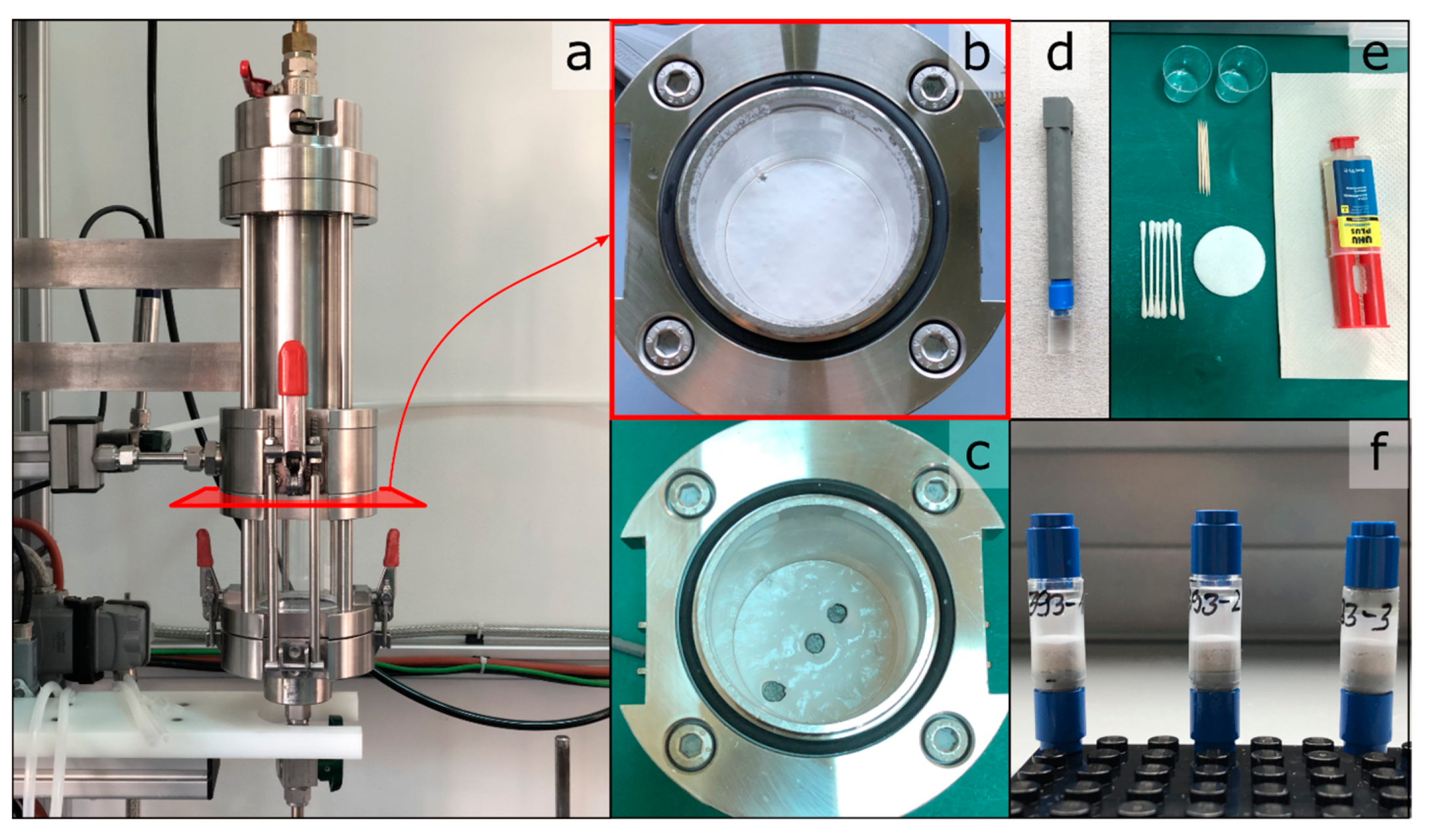
In this paper, the phantom technique is applied to filter cake structures. XRM offers an excellent opportunity in the field of liquid filtration research to investigate and describe prevailing mechanisms in filter cake formation and dewatering. Laboratory filtration experiments are often carried out in standardized test apparatuses, with resulting filter cakes having thicknesses in the range of a few centimeters. To obtain reliable results from XRM measurements for the whole filtration process, the entire height of a filter cake has to be considered. Data stitching of several individual scans covering certain areas of the filter cakes should be avoided in order to keep scanning time to a minimum, which in effect reduces drying and shrinking of the cake structures [21]. 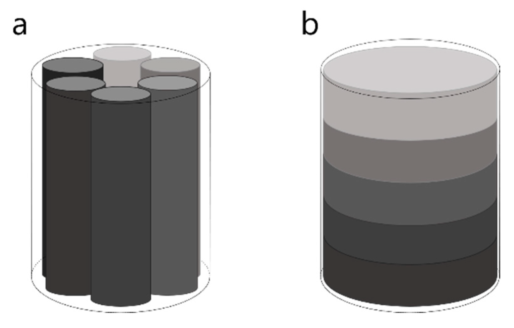With an appropriate FOV, the individual particles, whose sizes are usually in the µm range, cannot be resolved unless the size of the test apparatus itself is adjusted under certain assumptions [22]. In this case, however, it must be ensured that the experiment can be transferred to a smaller scale without the loss of information. If downscaling is not possible, a sampling technique will be required [23].

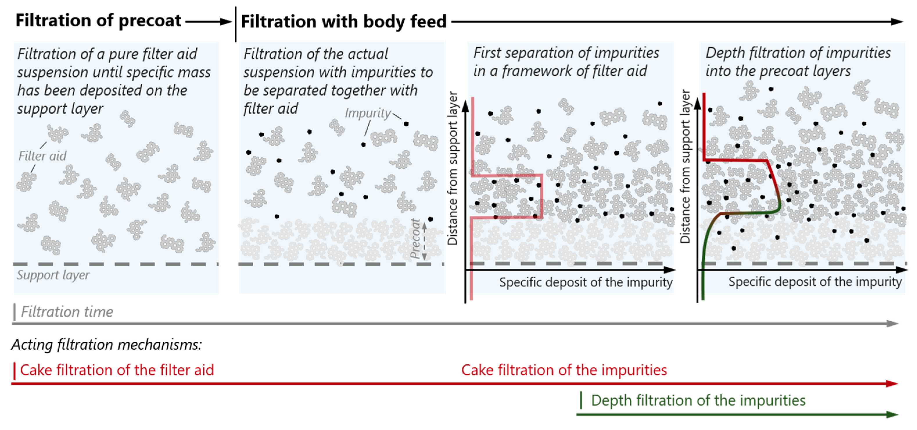
Filter aid filtration is a solid–liquid separation process. It is mainly applied for the separation of very fine particles below 5 µm from low concentrated suspensions which present considerable challenges for conventional filtration processes [24]. The aim is to obtain a particle-free filtrate as well as to build up a filter cake with a sufficiently high permeability. A filter aid is added to the suspension. The filter cake is therefore formed by the filter aid, with the impurities being deposited inside this cake. 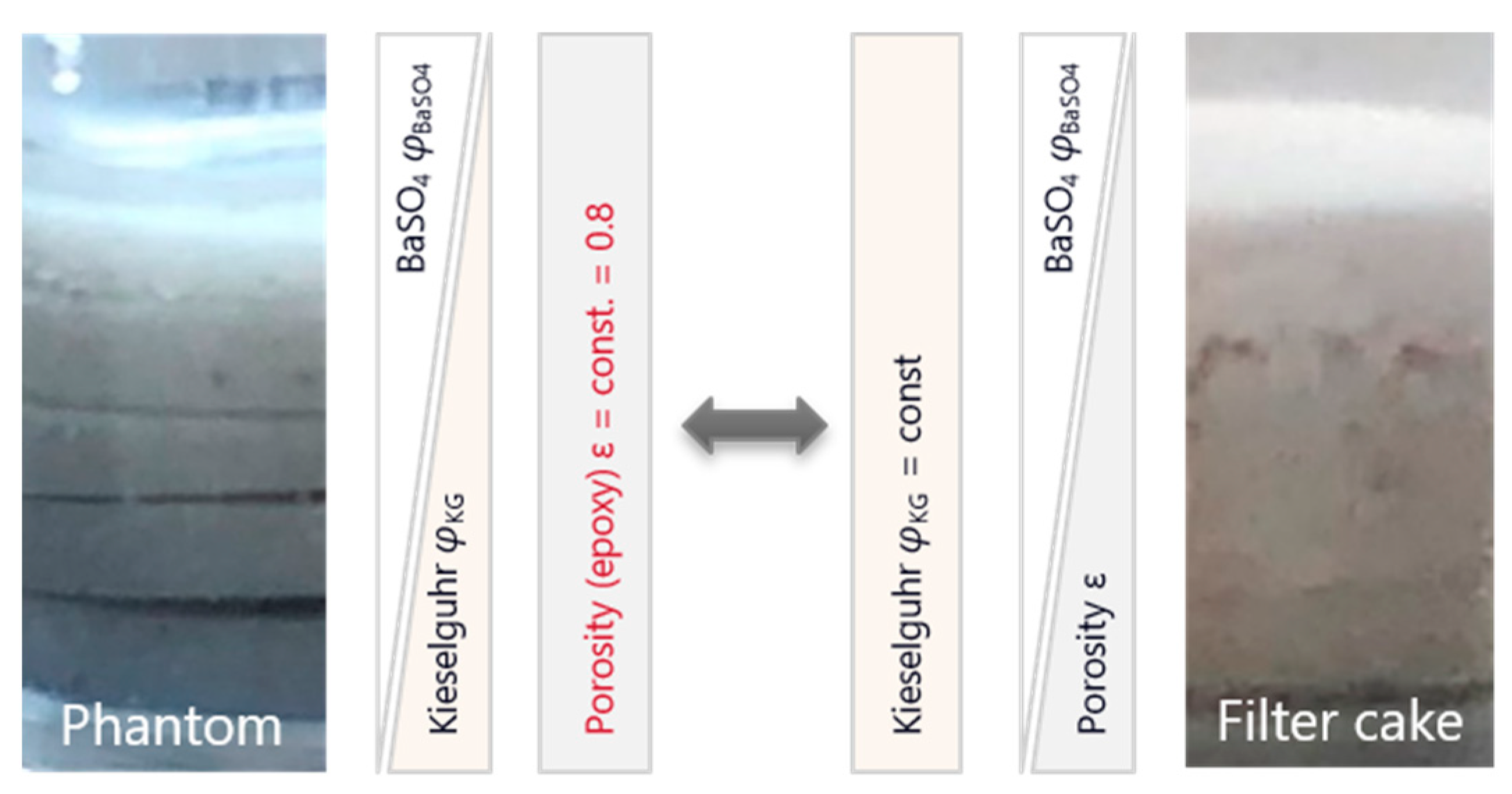Filter aid filtration can be achieved via several process strategies [25]. Our work focuses on the case of filter aid filtration with a precoat and a growing layer (see Figure 1). Here, a pure filter aid suspension is first filtered until a considerable amount of filter aid has been deposited on top of the support layer, forming a so-called precoat. The support layer is commonly a wire mesh with a relatively large aperture size, which in itself does not take part in the filtration of impurities at all. The precoat layer takes the functionality of the filter medium commonly used in filtration and is intended to protect against bleeding of impurities into the filtrate. After a precoat has been formed, the actual suspension containing the impurity is filtered together with the filter aid, comprising the so-called body feed.

In addition to the deposition of impurities in newly formed cake layers, transport of impurities into lower cake layers may take place [26,27]. Therefore, both cake filtration and depth filtration must be considered as taking place in the filter aid filtration process. In modeling the filtration process, it is important to have information about the fraction of impurity particles migrating into lower layers of the filter cake [28,29,30]. X-ray microscopy combined with the phantom calibration method offers the possibility of providing an insight into the impurity concentration profile if there is sufficient difference in X-ray attenuation between the filter aid and the impurity to be separated.

2. Materials and Methods

2.1. Material System

A model material system is chosen for its incompressible behavior during filtration. For this purpose, flux-calcinated kieselguhr Celite^® Hyflo Supercel is chosen as the filter aid. Kieselguhr ($\rho$ = 2.29 g/cm³), also known as diatomaceous earth, is a siliceous sediment derived from fossilized diatoms. Based on its application as a contrast agent in CT imaging [31], barium sulphate (BaSO₄, $\rho$ = 4.36 g/cm³) is used as a highly attenuating impurity. See

Table A1. Material properties of filter aid and impurity used for the filtration process.

	Kieselguhr, Flux Calcinated—Filter Aid	Barium Sulphate—Impurity
Material name	Celite® Hyflo Supercel	Barium sulfate puriss., Ph. Eur., BP
CAS No.	91053-39-3	7727-43-7
Supplier	Lehmann & Voss & Co.	Honeywell Fluka ™
Density ρ	2.29 g/cm3	4.36 g/cm3

of Appendix A for details regarding both particle systems. The particle size distributions of both materials are also given in Figure A1 of Appendix A. The suspension is created by mixing filter aid and impurity with deionized (DI) water.

2.2. Filtration

The filtration process is carried out on a laboratory filtration rig at constant flow rate. The filtration rig consists of a filtration cell, a scale, and a pressurized tank for the suspension. A schematic of the filtration setup is shown in Figure 2. The cake formation unit (CFU) has a diameter of 65 mm, resulting in an effective filtration area of 33.2 cm², and a volume of about 0.4 L. First, the precoat is built up on the support layer by cycling the suspension until a certain amount of filter aid is deposited on the support structure, immediately followed by the body feed filtration. During this process step, the volume flow is automatically kept constant by adjusting the pressure in the tank. In total, four filtration experiments are carried out using the same process parameters, which are summarized in

Table 1. Filtration parameters.

Precoat Filtration
Support layer (filter medium)		RPD 40 S (Reverse Plain Dutch Weave, pore size = 40 µm), Haver & Boecker
Specific precoat mass	${\mathit{m}}_{spec}$	1.5 kg filter aid per m2
Solid volume fraction of filter aid	${\mathit{\phi }}_{KG}$	0.44%
Mass flow suspension	${\dot{\mathit{m}}}_{susp}$	7.5 kg/h
Body Feed Filtration
Solid volume fraction of filter aid	${\mathit{\phi }}_{KG}$	0.046%
Solid volume fraction of impurity	${\mathit{\phi }}_{{BaSO}_{\mathbf{4}}}$	0.023%
Volume ratio	${\mathit{\phi }}_{KG}\mathbf{/}{\mathit{\phi }}_{{BaSO}_{\mathbf{4}}}$	2
Mass flow suspension	${\dot{\mathit{m}}}_{susp}$	5 kg/h

.

The filtration is stopped at a final filtrate mass of 10.5 kg. After filtration, the filter cake inside the CFU is dried at 60 °C for 30 min to remove the residual moisture on the filter cake surface. It is assumed that the entire pore volume of the cake is still filled with water at that point. After drying, three samples are taken from each filter cake, at radial positions of center, middle, and edge. The sample needs to be as small as possible while still ensuring proper handling and an unchanged cake structure. Plastic tubes, 15 mm in length and 8 mm in diameter, are used as the low X-ray attenuating sample containers. A tube is pushed gently into the filter cake and retracted containing the cake sample. In the following, the tube is sealed from below by gluing a piece of Lego^® on the base of the tube, which serves as the connector to the XRM sample holder. Figure 3 presents the workflow of the sample collection and further preparation.

With the FOV of the XRM measurement covering the whole sample, the minimum voxel size that can be achieved is 12 µm. As already mentioned, the spatial resolution is assumed here as five times the voxel size; thus, 60 µm. The individual BaSO₄ particles and approximately 88% of the kieselguhr particles, as indicated in Figure A1 of Appendix A, can therefore not be fully resolved on a particle level. As a consequence, image segmentation into the distinct features of impurity, filter aid, and pore space (DI water) is not possible when trying to obtain quantitative values about the composition of the filter cake.

2.3. Phantom Preparation

2.3.1. Preliminary

The preparation of the phantoms requires several assumptions to be considered. In addition to general requirements of the phantom method itself, both the filter cake and the XRM provided several boundary conditions. The phantom sample must contain all material phases of the original system. In our case, the original sample—the filter cake—consisted of kieselguhr, BaSO₄ and DI water. However, the sample must be stable during image acquisition to minimize the occurrence of motion artefacts in the resulting tomographic reconstruction. Such a stable phantom cannot be achieved when using water. Hill et al. [32] described additional disadvantages of liquid phantoms. Thus, a two-component epoxy resin was chosen as a substitute for DI water. The chosen epoxy was stable during X-ray irradiation and possessed a similar density to water. Furthermore, the epoxy resin proved to be a suitable substitute for the DI water regarding the ability to attenuate X-rays. Finally, the contained phases should be homogenously distributed within the phantom to ensure a constant grey value in the reconstructed volume. Therefore, thorough mixing of the solids with the epoxy resin is necessary.

Because the phantom has to be imaged using the same acquisition conditions as the sample of interest, i.e., the filter cake, the dimensions and the material composition of the surrounding container of the phantom should match those of the filter cake sample. This in return will influence the possible preparation method and the setup of the phantom. Therefore, phantom samples were prepared in the same plastic tubes as the cake samples. In terms of the measuring setup, the phantom sample needs to be entirely within the FOV and should represent the full range of X-ray attenuation strengths to be expected in the filter cake sample. Therefore, it is necessary to build a sample which consists of several subsamples with varying content of BaSO₄. Many commercial micro-CT phantoms contain several inserts, which are placed next to each other with the same radial distance from the sample center [33] (see Figure 4a). Based on the small dimension of the phantom in this study, a vertically stacked phantom setup was chosen instead (see Figure 4b). This setup represents the expected structure of the filter cake more closely, where impurity content is supposed to vary over the height of the sample, but not radially.

The prepared phantom thus consisted of five vertically stacked layers prepared as individual subsamples. If the amount of impurities in the filter cake is to be quantified correctly from the grey values of the reconstructed tomographic image, the content of at least one phase needs to be constant in the three-phase system. If, for example, the amount of epoxy is kept constant throughout the phantom, a simple mixing rule can be used to determine the amount of impurities in a slice of cake, since the grey value should increase linearly with impurity content.

2.3.2. Preparation Methodology

Each subsample was prepared individually. First, BaSO₄ and kieselguhr mixtures were prepared with a rubber spatula by subsequently sweeping the powder mixture back and forth over a sheet of paper for 10 min. Beforehand, open surface structures and pores of the paper were closed by spreading kieselguhr over the paper and removing it again before mixing. The amount of stress exerted onto the particles was enough to break agglomerates and create sufficient dispersion without crushing bigger kieselguhr particles. Based on the presented method by Ditscherlein et al. [34], the dispersed particulate sample was embedded inside an epoxy resin with low shrinkage and good infiltration properties. The resin (EpoThin 2, Buehler) has a processing time of 60 min and a curing time of 9 h at room temperature. This ensures slow mixing of the powder with the resin to minimize the generation of air bubbles which would be entrapped inside the hardened sample.

Using the database of the National Institute of Standards and Technology [35], the linear attenuation coefficient can be calculated for various compounds (with known material composition) as a function of the radiation energy. Since the exact chemical composition of the resin was not known and the proportions of its components can vary considerably here, this approach was not possible. Instead, a sample of pure epoxy resin with DI water on top was scanned and showed that the DI water phase of the real system was represented by the epoxy resin very well, and no grey value deviation based on the substitution was expected (see Figure A2 in Appendix A).

Figure 5 shows the steps of the phantom preparation. For the sake of the preparation, the volume fraction of epoxy resin was targeted to be ${\phi }_{\mathrm{E}\mathrm{p}\mathrm{o}\mathrm{x}\mathrm{y}}$ = 80% in every subsample, ensuring the best possible mixing as well as stable samples that could be cut easily. The volume fraction ${\phi }_{\mathrm{E}\mathrm{p}\mathrm{o}\mathrm{x}\mathrm{y}}$ = 80% represents the average measured porosity of the filter cake. The epoxy mixture was placed inside the sample container to harden. After removing a slice from the top which contained the epoxy meniscus, a slice of about 1 mm was cut using a diamond cutting disc. The final phantom was created by stacking and fixating five layers into the container glued together with epoxy resin.

For evaluation purposes, five phantom samples were prepared to achieve a reasonable understanding of the statistical robustness of the preparation method. The targeted compositions of the phantom layers are stated in

Table 2. Targeted barium sulphate and kieselguhr volume fractions for each of the phantom layers.

Layer No.	${\mathit{\phi }}_{{BaSO}_4}$ in %	${\mathit{\phi }}_{Kieselguhr}$ in %
5 (top)	8.0	12.0
4	6.7	13.3
3	3.3	16.7
2	0.8	19.2
1 (bottom)	0	20

. The mixing ratio of BaSO₄ and kieselguhr in layer 4 equals the mixing ratio used when preparing the body feed suspension.

2.4. XRM Measurements

The CT measurements were performed using the Zeiss Xradia 510 Versa XRM (Carl Zeiss Microscopy Deutschland GmbH, Oberkochen, Germany). All measuring and reconstruction parameters are stated in

Table 3. Acquisition and reconstruction parameters for the XRM measurements.

Parameter	Value
Acquisition
Acceleration voltage (keV)	80
Power (W)	7
Exposure time (s)	5
Voxel size (µm)	12
Number of projections	1601
Angle range (°)	360
Optical magnification	0.4
Binning	2
Source filter	Zeiss standard low energy LE5
Reconstruction
Algorithm	Filtered back projection
Beam hardening correction	0.05
Smooth filter	0.5
Byte scaling	User-defined CT scale filter

. The parameter selection was based on the filter cake sample and remained unchanged throughout the measuring campaign. Based on these acquisition parameters, the scan time per sample was approximately 3 h with a single 1 h warmup of the X-ray source before consecutive scanning. All scan data were reconstructed using Zeiss Reconstructor Scout & Scan version 11.1.8043 (Carl Zeiss Microscopy Deutschland GmbH, Oberkochen, Germany). The raw detector signal (32-bit) was converted into a 3D dataset (16 bit) during reconstruction, where the floating-point values were transformed into integer greyscale values in a process called global byte scaling. For this conversion step, a user-defined filter was created using the instructions provided by Zeiss, the details of which are given in the following passage.

2.5. CT Scaling Procedure

The reconstruction of all datasets using a CT scale is necessary to be able to compare greyscale values of different scans. In medical applications, CT scaling is a common practice using the dimensionless Hounsfield unit (HU); air and water receive the pixel values −1000 and 0, respectively, at 12-bit image resolution [36]. In the Zeiss user-defined scaling, the selected maximum and minimum grey value will be different from those of the Hounsfield scale, ranging, because of the 16-bit resolution of the tomogram, from 0 to 216. In order to create and use the scaling filter, a suitable scaling phantom needs to be scanned with the same parameters as the future samples. These parameters include the acceleration voltage, the lens, and the source filter. During reconstruction, the beam hardening coefficient must be the same as well. For this study, the phantom with the highest range in floating-point attenuation values is chosen as the scaling phantom. The lowest attenuating phase is the surrounding air (density = 0) and the highest attenuating phase is the phantom layer with the highest volume content of BaSO₄ (density = 15,000). The density value of the filter refers to the grey value after reconstruction using a scaling filter. After scaling, voxels in the cake with a stronger attenuation than those in the phantom layer with highest BaSO₄ volume fraction can still be represented with an individual grey value higher than 15,000.

Figure 6 shows the grey value over sample height for the reconstructed dataset using global byte scaling (b) and the CT scale filter (c). When the CT scale filter is used, the grey value plots align well, especially in the region of the lowest attenuating layers and in the plastic parts of the adjacent sample holder (below the dashed line). As expected, the plots show a step function, where each phantom layer possesses a constant grey value. The transition from one layer to the next can be seen as an abrupt change in grey value. A local minimum of grey values in between two phantom layers can be explained by geometric deviations during phantom preparation. As will be shown later, these discontinuity points are by no means critical for the further evaluation procedure. Based on these curves, the slice range for each layer was manually extracted from the dataset. This is a time-consuming but necessary procedure in order to extract the grey values of an area that is as unaffected by artefacts as possible.

2.6. Image Processing and Analysis

Processing and image analysis were performed using Fiji ImageJ Version 1.51w. The datasets reconstructed using the CT scale filter were exported as vertical stacks of images in TIFF format. No image post-processing, usually performed to improve image quality, was carried out as this would change the grey value histogram of each slice. In order to simplify and automate the analysis of the datasets, an ImageJ macro was used. The macro starts with creating a virtual subsample by selecting a region of interest from which statistical measures of the present grey value distribution, such as the mean value and the standard deviation, are determined. The occurrence of air entrapments inside filter cake samples or phantoms changes the mean grey value of each affected slices in the tomogram. As part of the error evaluation, the fraction of entrapped air is calculated for each image of the stack after segmentation using a second ImageJ macro. Here, a stack of binarized images was processed by dividing the number of pixels of entrapped air by the total number of pixels in each image.

3. Results

3.1. Calibration Curve

As can be seen in Figure 7a, the grey value of each extracted layer is plotted against the corresponding volume fraction of BaSO₄. This was performed for all five phantoms. Each layer is represented by a minimum number of 160 points in the case of layer 5 and more than 200 data points for all other layers. There are fluctuations in all five layers. However, they are more pronounced for the upper two layers, where the grey values of said layers even overlap. As can be seen in Figure 6, phantom image data show artefacts at the upper end of layer 5 that have a significant impact on the grey value histogram. Due to the location of layer 5 in the uppermost position, with the longest distance from the beam axis, the cone beam artefact leads to distortions and dark streaks in sideview.

For the linear fit, the data from all five phantoms were combined for each of the layers. Figure 7b shows a boxplot for each subsample. The artefacts of layer 5 are visible for all phantoms and lead to a significant broadening of the grey value distribution, especially towards lower grey values, which can clearly be seen when comparing the boxplots. Without the broadening towards lower grey values, the data of layer 5 would continue the trend. Nevertheless, the fifth layer is excluded from the determination of the linear fit.

In

Table 4. Statistical parameters for the five phantom layers based on the mean values from each of the 25 subsamples.

Layer No.1	1	2	3	4	5
Mean GV	3284.5	4661.8	8617.1	13,958.0	15,208.1
Std. deviation	93.5	50.0	144.2	175.1	448.5
Coeff. of variation (%)	2.9	1.1	1. 7	1.3	3.0

, mean value, standard deviation, and coefficient of variation of the grey value are calculated for each layer. The coefficient of variation is below 3% for layer 1 to 4. The higher value for layer 1 can be explained by the smaller absolute grey values in this layer.

The fit function approximates the data well and confirms the expected behavior of a linear relationship between impurity volume fraction and grey value for polychromatic X-ray sources. However, the linear fit describes the grey value as a function of barium sulphate volume fraction at constant epoxy volume fraction. The volume fraction of the third phase, kieselguhr, decreases with increasing BaSO₄ volume fraction. For the use as a calibration function, the relationship of grey value as a function of BaSO₄ volume fraction at constant kieselguhr volume fraction is needed, because the cake is expected to have a different structural setup compared to the phantom. In the cake, the volume fraction of kieselguhr can be assumed to remain nearly constant, since the much smaller BaSO₄ particles will fill the interstices and inner porosity of the kieselguhr structures [37,38]. This in turn will lead to a decreasing porosity with increasing BaSO₄ content in the cake. Figure 8 shows a schematic comparison.

The linear fit can be described as the summation of the grey values of the pure phases weighted by their respective volume fractions:

$$G{V}_{\mathrm{total}}={\phi }_{{\mathrm{BaSO}}_4}\cdot G{V}_{{\mathrm{BaSO}}_4}+{\phi }_{\mathrm{KG}}\cdot G{V}_{\mathrm{KG}}+{\phi }_{\mathrm{Epoxy}}\cdot G{V}_{\mathrm{Epoxy}}$$

(2)

where $G{V}_{\mathrm{B}\mathrm{a}\mathrm{S}{\mathrm{O}}_4}$, $G{V}_{\mathrm{K}\mathrm{G}}$, and $G{V}_{\mathrm{E}\mathrm{p}\mathrm{o}\mathrm{x}\mathrm{y}}$ represent the grey value of the pure materials. From the scan of the pure epoxy sample, $G{V}_{\mathrm{E}\mathrm{p}\mathrm{o}\mathrm{x}\mathrm{y}}$ is determined. From the y-axis intercept of the linear fit representing the two-phase system of epoxy and kieselguhr, $G{V}_{\mathrm{K}\mathrm{G}}$ is calculated. The determination of the two grey values now permits the calculation of $G{V}_{\mathrm{B}\mathrm{a}\mathrm{S}{\mathrm{O}}_4}$. The calibration function is established for the assumption of constant kieselguhr volume fraction ${\phi }_{\mathrm{K}\mathrm{G}}=0.2$ over cake height and the interdependency of the remaining volume fractions: ${\phi }_{\mathrm{E}\mathrm{p}\mathrm{o}\mathrm{x}\mathrm{y}}=0.8-{\phi }_{\mathrm{B}\mathrm{a}\mathrm{S}{\mathrm{O}}_4}$.

$${\phi }_{{\mathrm{BaSO}}_4}=\frac{\left(G{V}_{\mathrm{total}}-0.2\cdot G{V}_{\mathrm{KG}}\right)-0.8\cdot G{V}_{\mathrm{Epoxy}}}{G{V}_{{\mathrm{BaSO}}_4}-G{V}_{\mathrm{Epoxy}}}$$

(3)

Equation (3) acts as the calibration function for the following quantitative analysis of the filter cake data.

3.2. Results of a Validation Filter Cake

In an additional filtration experiment, a validation filter cake was created and analyzed. Compared to the filter cakes created by combined precoat and body feed filtration, the composition of this one filter cake was precisely known as the fractions of the materials were adjusted beforehand. The kieselguhr and BaSO₄ volume fractions were chosen to be 20%, respectively, with the resulting porosity expected to be 60%. The BaSO₄ fraction was well above the highest one used for establishing the calibration function. This allowed us to check whether the extrapolated function would still be accurate for higher BaSO₄ fractions in the cake.

In this particular filtration setup, the filtration rig was used at constant-pressure operation and with direct feed. All solids were deposited inside the filter cake and no feed tank was necessary, as the total amount of suspension was added to the CFU before applying pressure. From the validation filter cake, a sample was taken and scanned according to the described procedures. Figure 9 shows the BaSO₄ volume fraction plot over distance from sample base for the validation filter cake. The validation filter cake shows an almost constant grey value over its sample height. It becomes clear that the calibration was successful: the mean BaSO₄ volume fraction of the validation cake, as stated from the calibrated CT data, is 18.3%, which in the suspension was adjusted to 20%. Based on the calibration assuming 20% of kieselguhr inside the filter cake, the resulting pore volume fraction would be 61.7%, which is somewhat smaller than the mean porosity determined experimentally (67.7%).

The additional filter cake is an important element to validate the methodology of the calibration and thus confirms the phantom as an adequate representation of the original system, even when using epoxy as substitute for DI water. In addition, the validation provides a statement on how accurately the calibration reproduces the volume fraction inside the filter cake. The difference between the two porosity values might not be a direct consequence of the calibration function itself. The influence of other factors is discussed in Section 4.2.

3.3. Quantitative Analysis of Filter Cakes

Figure 10 contains a dataset of an almost ideal filter cake sample without discernable artefacts such as air entrapments, cracks, or sample drift. The plot of the BaSO₄ volume fraction (Figure 10b) represents the total cake sample starting from 0 mm above the sealed sample base to the upper end of the filter cake at about 4.5 mm.

From the plot, a constant BaSO₄ volume fraction of 0% is observed between 0 mm and 2.5 mm, where the filter cake layers only consist of kieselguhr and pore space (DI water). During the filtration process, the BaSO₄ impurity particles are accumulated within the body feed layers or are retained in upper precoat layers by depth filtration. No BaSO₄ particles were able to pass the precoat; thus, the filtrate remained clear during the experiments. Starting at 2.5 mm, the increasing BaSO₄ volume fraction reaches a plateau at 3.5 mm, indicating the peak of separated impurity. With increasing sample height, the volume fraction begins to decrease. A final rapid decrease marks the top end of the sample. As a consequence of the calibration function, the volume fraction becomes negative due to the grey value of air, which is lower than that of the phantom layer representing 0% BaSO₄.

Grey value over distance from the sample base is plotted in Figure 10c for a filter cake sample after filtration of only filter aid (kieselguhr) without impurity. The grey values of the dataset were not transferred using the calibration function because the sample was imaged slightly differently due to its height of over 6 mm. Nevertheless, it acts as a principle reference. The grey value is constant over the whole sample height, confirming the uniform structure of the filter cake built by only kieselguhr particles.

4. Discussion

4.1. Assessment of the Quantitative Analysis

Qualitatively, the plot is in very good agreement with the simulation results based on the mechanistic model by [29], which describes the process of precoat and body feed filtration. Moreover, the assumption of a filter cake pore fraction of 80% in the precoat—which was adjusted to be the volume fraction of epoxy in the phantom—is correct. For the description of the specific deposition behavior and the filtration effects, it is important to combine results from simulation with quantitative characterization. Especially in the transition area between layers produced by precoat and body feed filtration, the increase in BaSO₄ volume fraction should be captured as precisely as possible. After the filtration experiments, the cake height is determined by measurements of the distance between the top of the cake formation unit (CFU) and the filter cake surface. Those values are then subtracted from the total height of the CFU. As the cake height is subject to variation, the measurement is performed at five positions on the filter cake surface. For comparison, the cake height is also determined from the reconstructed 3D filter cake. The manually measured and computed heights differ for all of the samples. For some samples, cake residue, which stuck to, and therefore remained on, the surface of the filter medium during sampling seems be the reason for the difference. Details regarding the difference in cake height are stated in

Table A2. Mean measured cake height in mm and cake height based on CT measurements in mm for all cake samples from experiments 1 to 4 with positions center (C), middle (M), edge (E).

Experiment	1			2			3			4
	C	M	E	C	M	E	C	M	E	C	M	E
hmeas in mm	5.5			5.6			5.9			5.8
hCT in mm	4.8	5.1	4.9	4.8	5.0	4.5	4.8	5.2	5.2	3.8	4.3	4.6

of Appendix A. For the chosen filter cake presented in Figure 10, the average height difference is 0.5 mm. From five separate experiments, the average precoat height is 3.2 mm. Assuming the sampling procedure to be the only reason for the height difference, the transition zone (precoat/body feed) is located at around 2.7 mm. For the plot in Figure 10, this means that there is little transport of impurity into the precoat, which contradicts the previous assumptions that the maximum impurity concentration is found in the transition zone [29].

The amount of impurity particles separated inside the body feed filter cake layers by means of depth filtration can be estimated by mass balance of the feed materials. From the data of the pure filtration experiment (Figure 10c), the kieselguhr filter cake has a uniform structure with porosity of ${\phi }_{\mathrm{E}\mathrm{p}\mathrm{o}\mathrm{x}\mathrm{y}}$ = 80% and a corresponding kieselguhr volume fraction of ${\phi }_{\mathrm{K}\mathrm{G}}$ = 20%. As stated before, for filtration at constant volume flow it is generally accepted that the filter aid will form a rigid cake whose structure remains unaffected by the impurity particles during the body feed filtration [39]. In fact, BaSO₄ particles will be held back by the kieselguhr structures and accumulate inside the pore space. As a consequence, the pore volume fraction will decrease in those parts of the filter cake with higher BaSO₄ deposition. Based on the mixing ratio of kieselguhr and BaSO₄ in the body feed suspension, the BaSO₄ volume fraction should be half that of kieselguhr. Under the condition that the suspension reaches the CFU with the same ratio of kieselguhr and BaSO₄ prepared in the feed tank (Table 1), a body feed layer built up by cake filtration only would consist of 20% kieselguhr, 10% BaSO₄, and 70% pore space. Any layer in the analyzed filter cake sample with a BaSO₄ volume fraction exceeding 10% would contain BaSO₄ transported through the cake by depth filtration from the above cake layers.

The quantitative values of the body feed layers of Figure 10b should be questioned, as they show an increasing amount of BaSO₄ throughout the body feed layers. Peak BaSO₄ volume fractions of up to 20% are reached, which is twice the amount expected for the body feed without depth filtration. The higher amount of BaSO₄ is likely the result of depth filtration, but both density separation and particle inertia during the transport of the body feed suspension to the cake formation unit might also play a role. As can be seen in the schematic of the filtration apparatus (Figure 2), the dip tube, through which the suspension is pushed into the cake formation unit by the pressurized air, is installed vertically. Since the anchor impeller in the tank primarily causes a tangential movement of liquid, the dip tube is thus oriented perpendicular to the main direction of flow. The smaller BaSO₄ particles will enter the tube more easily, since their inertia is not as strong as that of the kieselguhr particles, which, because of their high porosity, will basically act as a continuum with the liquid phase. Because of the higher density, BaSO₄ will additionally tend to accumulate at the bottom of the pressurized tank, in effect leading to an increased mass fraction in the vicinity of the dip tube. The setup may ultimately lead to a much higher fraction of BaSO₄ transported to the cake formation unit than expected and the overall higher content inside the cake.

4.2. Error Evaluation

4.2.1. Filtration

The filter aid filtration was repeated four times at the same conditions. Looking at the reproducible process data in Figure 11, there is no significant deviation in process pressure and volume flow. No outliers are detected. The volume flow fluctuates because of the system control, especially in the beginning of the experiments, where the control system needs to settle. However, these fluctuations are prominent in all experiments.

As can be seen in Figure 12, three samples (center, middle, edge) were taken from each of the four filter cakes and scanned in the XRM, as described in Section 2.2. The grey value plots are aligned at the top and thus the upper end of the cake sample, because, as described before, the total sample height was influenced by the sampling procedure. The deviation between grey value profiles of a single experiment is very small, which is indicated by the mean BaSO₄ volume fraction (shown as a dashed red line in Figure 12).

For experiment 3 and 4, the deviation between mean grey values is more pronounced than for experiments 1 and 2, especially from −2 mm to −1 mm, where the transition from precoat to body feed filtration resulted in an increased number of air inclusions caused by switching the piping from precoat to body feed filtration. The air inclusions vary in size and position, but it is assumed that they are more or less evenly distributed over the filtration area. Their extent can best be investigated by looking at specific slices in XRM data of the samples.

Figure 13 shows three slices from the reconstructed filter cake sample 1 (edge) and 4 (edge). Sample 1 (edge) shows only a few air inclusions that mainly occur in the transition zone. For sample 4 (edge), the air inclusions are also present inside the precoat and the transition zone, where much larger air inclusions appear as well. For all the samples, no inclusions are detected inside the body feed cake layers. The presence of these big air inclusions in sample 4 affects the grey value in the slices where they are present. Due to the low attenuation of air, the grey value is falsely reduced. Using an ImageJ macro on binarized datasets, the fraction of air inclusions of the slices’ total area is computed.

In Figure 14, the fraction of air inclusions in the sample slices is plotted for each filtration experiment. There are only a few air inclusions in the lower and upper areas of the filter cake samples. Bigger air inclusions right at the beginning of the sample (−4 to −3 mm, depending on the sample) derive from sampling, where, during the sealing of the sample, air may have become trapped. In the middle of the filter cake, inclusions mark the transitions between the precoat and body. For experiments 1 and 2, the maximum amount of air inclusion per unit area is 5 to 10%, while for experiments 3 and 4 this increases to values of 15% and 20%, respectively. The deviation in grey value is approximately equal to the fraction of air, since the air’s grey value is close to zero. However, the exact quantification is more difficult. Selecting a threshold for excluding the air inclusions during the calculation of the mean grey value is not possible for a whole dataset of a filter cake. The grey value of the air inclusions depends on their location and is lower in the precoat than in the body feed. When calculating the BaSO₄ volume fractions, absolute differences of 1 to 2% would result for ${\phi }_{{\mathrm{BaSO}}_4}$. The relative deviation depends on the position of the analyzed slice within the filter cake and is higher for the precoat, where the overall grey value is lower.

Air inclusions smaller than the spatial resolution cannot be resolved, and are therefore not considered in the determination of the air inclusions. However, their influence is expected to be negligibly small. Furthermore, Perera et al. [40] write that the surface of diatomaceous earth is very well wetted by water due to hydrophilic silanol groups. From this, it can be assumed that open and permeable pores are completely filled with water during filtration. This assumption is emphasized by the low content of air inclusions in the precoat layers. In each of the four experiments, the three sampling positions are representative for the total filter cake. In addition, a homogenous deposition of BaSO₄ over the entire area of the cake formation unit can be assumed without significant local enrichment.

4.2.2. Phantom

Similar to the filter cake samples (Figure 13), the review of the tomography raw data of the phantoms already revealed unwanted air inclusions in the phantom layers. The analysis of the amount of air inclusions shows that for the phantoms the amount is more or less constant over the phantom height within a range of 0 to 7% (see Figure 15) with a mean value of approximately 4%.

Peaks in the grey value profile can be attributed to the slices that belong to the transitions between the layers, which are glued together but can still contain entrapped air. The amount of air inclusions in the phantoms is only half to a quarter of the fraction in strongly affected filter cake areas.

Note that the viscosity and wettability of the epoxy resin are not known, which makes it difficult to say whether the fine kieselguhr pores are filled with the resin. Due to the mechanically stable resin matrix, it was possible to prepare vertically polished cuts and produce scanning electron microscopy (SEM) images with a much higher lateral resolution than the XRM. The images presented in Figure 16 give a good first impression of the pore fill state.

The kieselguhr pores possess the same grey value as the background. Because the samples are not re-embedded after polishing, the epoxy present in the pores stems from the original sample preparation. The influence of unfilled pores is therefore negligible. When looking at the SEM images, it becomes obvious that the homogeneity of the solids dispersed in the epoxy may not be sufficiently high (see Figure 16b), which leads to an undesired grey value distribution. However, in most cases, the effect is minimized due to the PVE at lower XRM resolutions and compensated by averaging the grey values for each slice.

Hill et al. [32] describe which effects can cause spatial inhomogeneity in epoxy resin-based samples. These include, in particular, insufficient mixing of the components and segregation effects, for example, due to sedimentation or aggregation of particles. Sedimentation of kieselguhr and BaSO₄ cannot be disregarded completely. As explained in the methods section, during sample preparation, the meniscus of each subsample is removed, after which a 1 mm thick slice is cut off and used in the phantom. A cause for error could be the deviation of the proportions of materials in the cut-off disc from the fraction adjusted for by weighing each material. However, the resolution of the SEM is not high enough to analyze the area fractions of each material, because, especially, some of the BaSO₄ particles are smaller than the SEM’s resolution.

Instead, the remaining part of a phantom subsample (layer 5 of phantom 5) was scanned in the XRM. Figure 17 shows the resulting grey value plot of the subsample as well as that of phantom 5. It is clear that no sedimentation of the solids took place before the epoxy resin hardened, because the grey value is constant over the remaining subsample’s height. Furthermore, the grey value of the subsample is identical to the grey values of layer 5 of phantom 5, again confirming the homogeneity of the subsample. In summary, the main error source in the preparation of the phantom is the mixing of the solid phases with the epoxy resin, which may lead to both air inclusions and an inhomogeneous distribution of solids.

4.2.3. XRM

Consequently, the influence of artefacts arising from the three-dimensional imaging by XRM is discussed. Due to the polychromatic X-ray spectrum, beam hardening will always be present to some extent [4]. However, the application of energy-dependent filters can reduce this effect significantly. Additionally, during reconstruction, a beam hardening correction is applied. Based on its dependency on solid density and atomic number, the X-ray attenuation can be very different in certain areas of the filter cake: the precoat will attenuate ever so slightly, with the body feed layers leading to high attenuation because of the BaSO₄ content. This makes it hard to choose both the filter and the factor for the beam hardening correction that fit both cake areas and the different phantom layers. The chosen beam hardening correction factor is rather low. After reconstruction with the CT scale filter and the beam hardening correction, no cupping effect, and thus no obvious beam hardening, is detected. The procedure revealed that surrounding areas (air inclusions) of highly attenuating structures (body feed layers) might be represented by a higher grey value. An erroneous increase of the grey value in surrounding areas of contrast agent has been observed [41]. Despite automatic ring removal during acquisition, some ring artefacts can be observed. Other nonlinear effects might arise and affect the grey value of voxels that are also subject to the PVE. Any nonlinear effects would be especially prominent in the sample areas located furthest from the cone beam center.

5. Conclusions

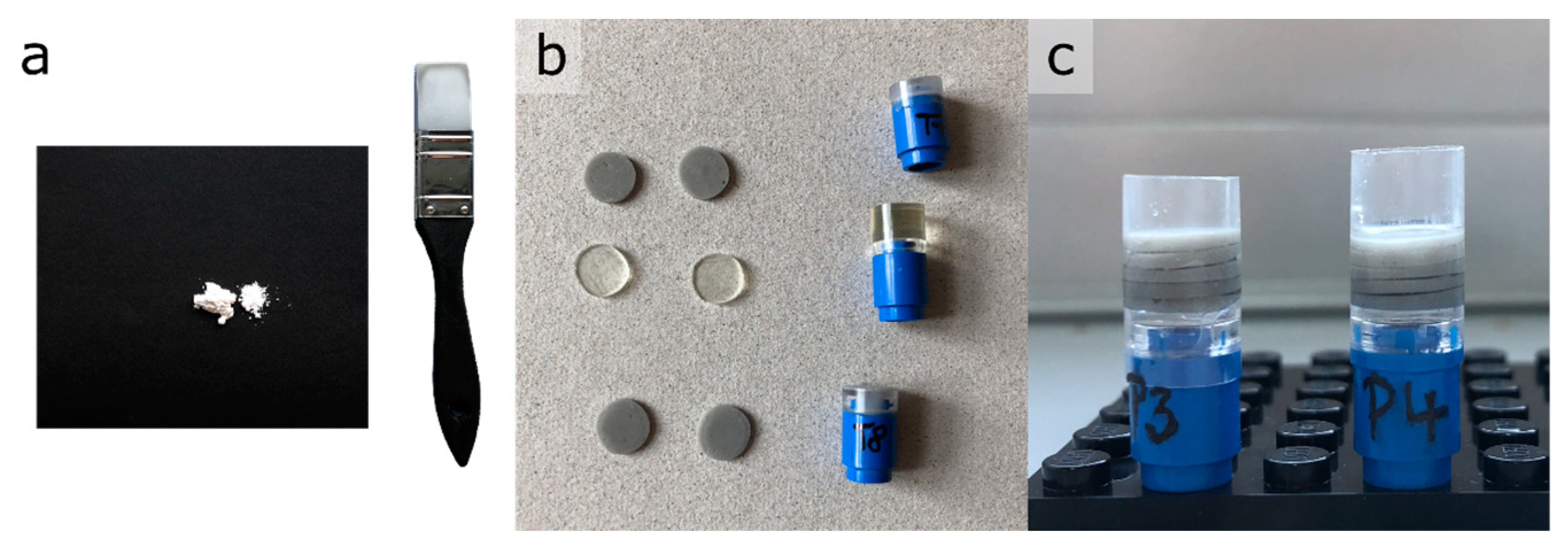
The phantom calibration method is applied to the three-dimensional filter cake characterization using X-ray microcomputed tomography with the aim of determining the amount of separated impurity inside a filter cake. This in turn allows for the quantification of filtration effects. An approach using a calibration in CT imaging is necessary as the particles of interest, especially the impurity particles, are much smaller than the maximum possible spatial resolution of the measuring setup. As a consequence, segmentation into distinct phases of filter aid, impurity, and pore volume and a following quantitative analysis are not feasible.

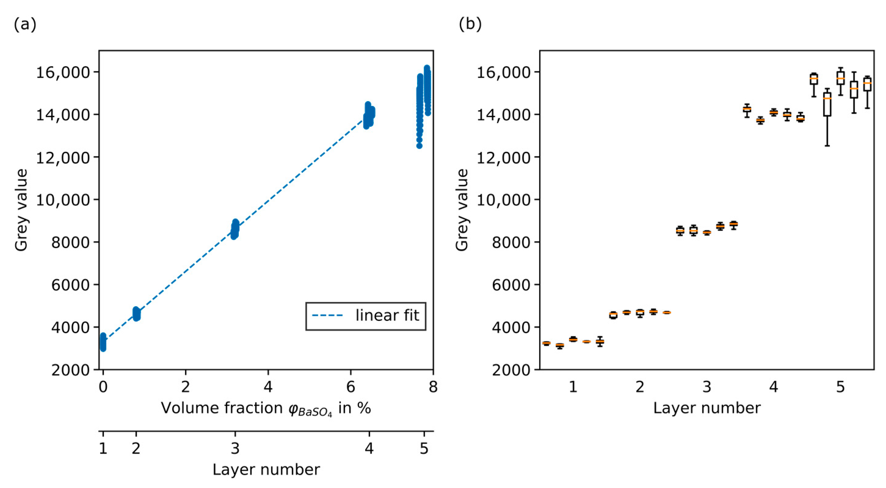
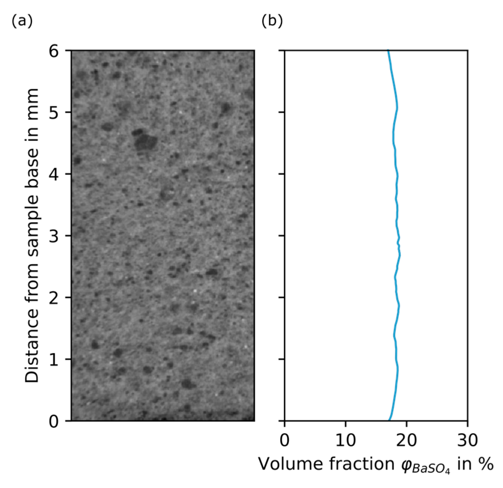
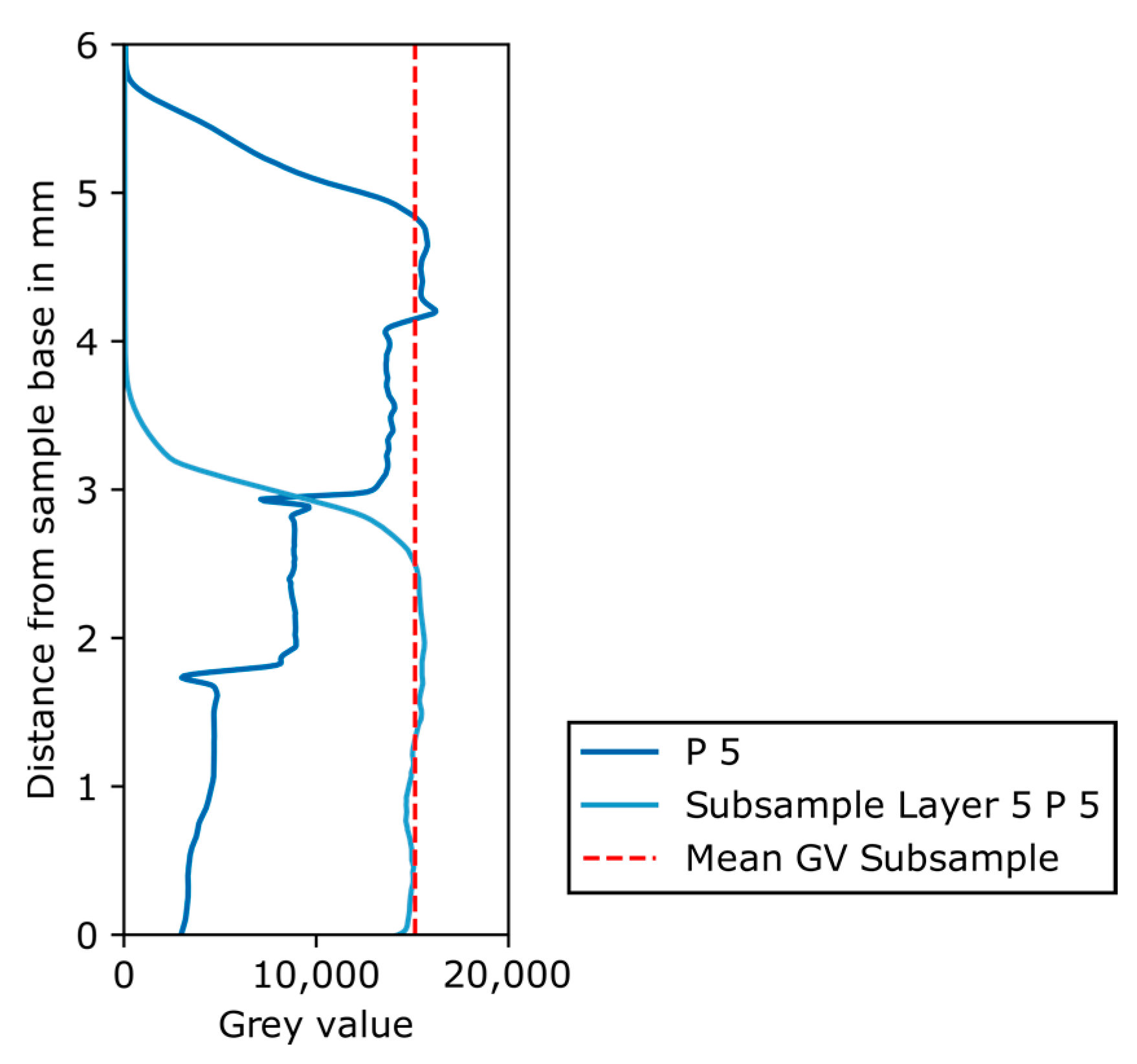
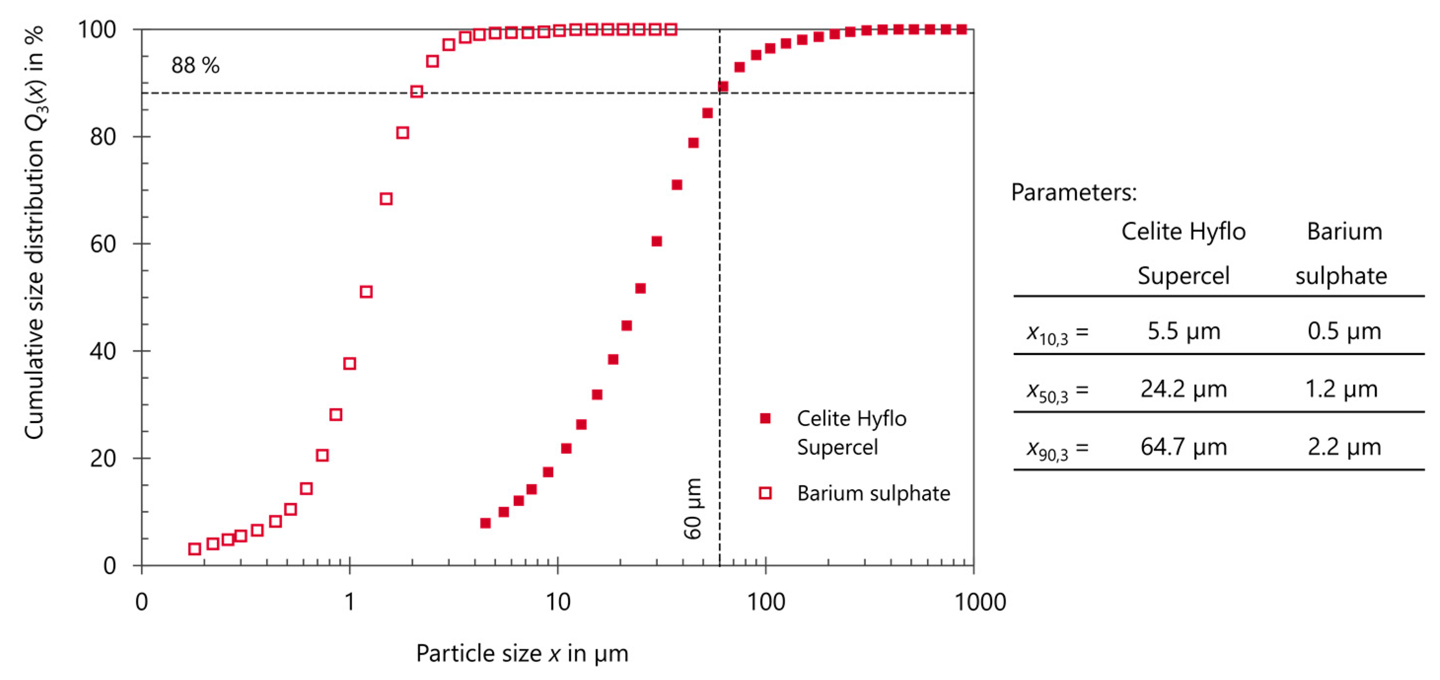
Kieselguhr is used as the filter aid and barium sulphate acts as an impurity substance. The grey values of prepared phantoms are correlated with the corresponding BaSO₄ volume fraction. The thereby acquired calibration function is used to transfer the grey values of the filter cake datasets into BaSO₄ volume fractions, which allow further analysis. The validation confirms the correctness of the calibration function.

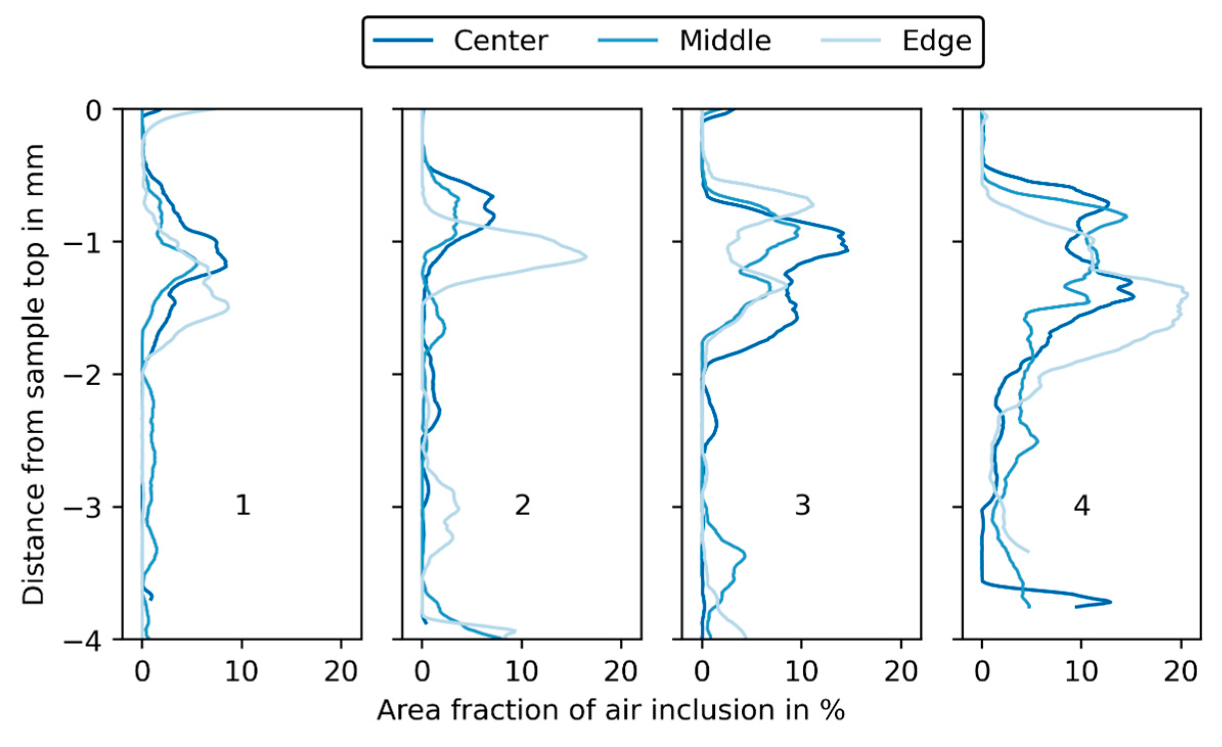
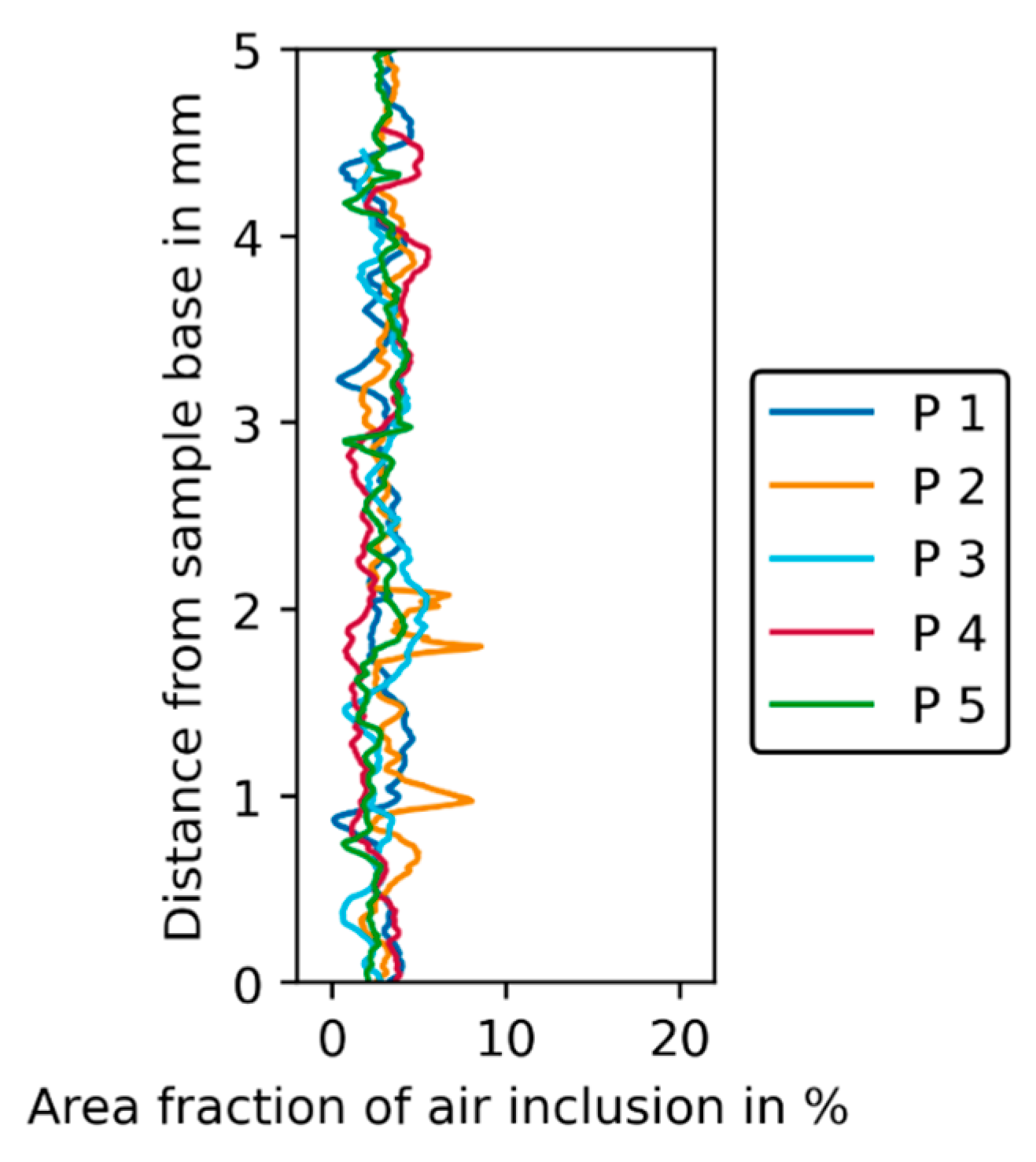
The tested approach is new in the field of filter cake characterization. It is promising and delivers reproducible and valid results for the filter cakes prepared in constant volume flow experiments, with precoat and body feed layers. The resulting BaSO₄ volume fractions are higher than anticipated beforehand, indicating that the filtration process using a pressurized tank influences the composition of the feed suspension. After evaluating all experimental parts, the significance of many possible influences is ruled out. Only the occurrence of air inclusions is expected to influence the resulting impurity volume fractions. The occurrence of imaging artefacts should not be underestimated but could be kept to a minimum and is ruled out as a significant factor here.

A positive outlook is drawn as the presented work shows the immense value of additional information by exploiting subvoxel data. An extension towards the quantification of two different impurities in a simplified system should be possible with the described methodology, provided the contents of all other phases in the system are known. Filtration effects can now be studied in more detail for a wider range of experimental setups with different process parameters.

References

1. Buzug, T.M. Computed Tomography: From Photon Statistics to Modern Cone-Beam CT; Springer: Berlin/Heidelberg, Germany, 2008. [Google Scholar]
2. Englisch, S.; Ditscherlein, R.; Furat, O.; Hansen, L.; Drobek, D.; Wirth, J.; Carl, S.; Leißner, T.; Zubiri, B.A.; Weber, A.; et al. Comprehensive, multidimensional and correlative particle characterization of a saxolite and talcum compound to support the understanding of complex separation processes. Microsc. Microanal. 2021, 27, 934–937. [Google Scholar] [CrossRef]
3. Löwer, E.; Pfaff, F.; Leißner, T.; Peuker, U.A. Neighborhood Relationships of Widely Distributed and Irregularly Shaped Particles in Partially Dewatered Filter Cakes. Transp. Porous Media 2021, 138, 201–224. [Google Scholar] [CrossRef]
4. Cnudde, V.; Boone, M.N. High-resolution X-ray computed tomography in geosciences: A review of the current technology and applications. Earth-Sci. Rev. 2013, 123, 1–17. [Google Scholar] [CrossRef]
5. Wellington, S.L.; Vinegar, H.J. X-Ray Computerized Tomography. J. Pet. Technol. 1987, 39, 886–898. [Google Scholar] [CrossRef]
6. Clausnitzer, V.; Hopmans, J.W. Pore-scale measurements of solute breakthrough using microfocus X-ray computed tomography. Water Resour. Res. 2000, 36, 2067–2079. [Google Scholar] [CrossRef]
7. Boas, F.; Fleischmann, D. CT artifacts: Causes and reduction techniques. Imaging Med. 2012, 4, 229–240. [Google Scholar] [CrossRef]
8. Withers, P.J.; Bouman, C.; Carmignato, S.; Cnudde, V.; Grimaldi, D.; Hagen, C.K.; Maire, E.; Manley, M.; Du Plessis, A.; Stock, S.R. X-ray computed tomography. Nat. Rev. Methods Prim. 2021, 1, 18. [Google Scholar] [CrossRef]
9. Zhang, Y.; Mostaghimi, P.; Armstrong, R.T. On the challenges of greyscale-based quantifications using X-ray computed microtomography. J. Microsc. 2019, 275, 82–96. [Google Scholar] [CrossRef]
10. Bailey, J.J.; Heenan, T.M.M.; Finegan, D.P.; Lu, X.; Daemi, S.R.; Iacoviello, F.; Backeberg, N.R.; Taiwo, O.O.; Brett, D.J.L.; Atkinson, A.; et al. Laser-preparation of geometrically optimised samples for X-ray nano-CT. J. Microsc. 2017, 267, 384–396. [Google Scholar] [CrossRef]
11. Maire, E.; Withers, P.J. Quantitative X-ray tomography. Int. Mater. Rev. 2013, 59, 1–43. [Google Scholar] [CrossRef]
12. Bruns, S.; Stipp, S.L.S.; Sørensen, H.O. Statistical representative elementary volumes of porous media determined using greyscale analysis of 3D tomograms. Adv. Water Resour. 2017, 107, 32–42. [Google Scholar] [CrossRef]
13. Xu, X.G. An exponential growth of computational phantom research in radiation protection, imaging, and radiotherapy: A review of the fifty-year history. Phys. Med. Biol. 2014, 59, R233–R302. [Google Scholar] [CrossRef] [PubMed]
14. Cann, C.E.; Genant, H.K. Precise measurement of vertebral mineral content using computed tomography. J. Comput. Assist. Tomogr. 1980, 4, 493–500. [Google Scholar] [CrossRef] [PubMed]
15. Free, J.; Eggermont, F.; Derikx, L.; van Leeuwen, R.; van der Linden, Y.; Jansen, W.; Raaijmakers, E.; Tanck, E.; Kaatee, R. The effect of different CT scanners, scan parameters and scanning setup on Hounsfield units and calibrated bone density: A phantom study. Biomed. Phys. Eng. Express 2018, 4, 055013. [Google Scholar] [CrossRef]
16. De Marzi, L.; Lesven, C.; Ferrand, R.; Sage, J.; Boule, T.; Mazal, A. Calibration of CT Hounsfield units for proton therapy treatment planning: Use of kilovoltage and megavoltage images and comparison of parameterized methods. Phys. Med. Biol. 2013, 58, 4255–4276. [Google Scholar] [CrossRef]
17. Üncü, Y.A.; Sevim, G.; Canpolat, M. Approaches to preclinical studies with heterogeneous breast phantom using reconstruction and three-dimensional image processing algorithms for diffuse optical imaging. Int. J. Imaging Syst. Technol. 2022, 32, 343–353. [Google Scholar] [CrossRef]
18. Rahn, H.; Alexiou, C.; Trahms, L.; Odenbach, S. 3-Dimensional quantitative detection of nanoparticle content in biological tissue samples after local cancer treatment. J. Magn. Magn. Mater. 2014, 360, 92–97. [Google Scholar] [CrossRef]
19. Darma, I.S.; Sugiyama, T.; Promentilla, M.A.B. Application of X-Ray CT to Study Diffusivity in Cracked Concrete Through the Observation of Tracer Transport. J. Adv. Concr. Technol. 2013, 11, 266–281. [Google Scholar] [CrossRef]
20. Molnar, I.L.; Willson, C.S.; O’Carroll, D.M.; Rivers, M.L.; Gerhard, J.I. Method for obtaining silver nanoparticle concentrations within a porous medium via synchrotron X-ray computed microtomography. Environ. Sci. Technol. 2014, 48, 1114–1122. [Google Scholar] [CrossRef]
21. Pham, T.H.; Peuker, U.A. Shrinkage Cracking During Filtration Experiments—Influence of Suspension Concentration on Crack Formation. In Proceedings of the International Conference on Innovations for Sustainable and Responsible Mining; Springer: Cham, Switzerland, 2021; pp. 385–406. [Google Scholar]
22. Löwer, E.; Leißner, T.; Peuker, U.A. Insight into filter cake structures using micro tomography: The dewatering equilibrium. Sep. Purif. Technol. 2020, 252, 117215. [Google Scholar] [CrossRef]
23. Du Plessis, A.; Boshoff, W.P. A review of X-ray computed tomography of concrete and asphalt construction materials. Constr. Build. Mater. 2019, 199, 637–651. [Google Scholar] [CrossRef]
24. Sutherland, D.N.; Hidi, P. An Investigation of Filter-Aid Behaviour. Trans. Instn. Chem. Engrs. 1966, 44, T122–T127. [Google Scholar]
25. Hackl, A.; Heidenreich, E.; Höflinger, W.; Tittel, R. Filterhilfsmittelfiltration. Fortschr.-Ber. VDI Reihe 3 Nr. 348; VDI-Verlag: Düsseldorf, Germany, 1993. [Google Scholar]
26. Heertjes, P.M.; Zuideveld, P.L. Clarifications of Liquids Using Filter Aids. Part II. Depth Filtration. Powder Technol. 1978, 19, 31–43. [Google Scholar]
27. Tien, C.; Bai, R.; Ramarao, B.V. Analysis of cake growth in cake filtration: Effect of fine particle retention. AIChE J. 1997, 43, 33–44. [Google Scholar] [CrossRef]
28. Kuhn, M.; Briesen, H. Dosage of Filter Aids in the Case of Pure Surface Filtration—An Optimal Control Approach. In 12th International Symposium on Process Systems Engineering and 25th European Symposium on Computer Aided Process Engineering; Gernaey, K., Huusom, J., Gani, R., Eds.; Elsevier: Copenhagen, Denmark, 2015. [Google Scholar]
29. Kuhn, M.; Briesen, H. Dynamic Modeling of Filter-Aid Filtration Including Surface- and Depth-Filtration Effects. Chem. Eng. Technol. 2016, 39, 425–434. [Google Scholar] [CrossRef]
30. Kuhn, M.; Kirse, C.; Briesen, H. Improving the design of depth filters: A model-based method using optimal control theory. AIChE J. 2018, 64, 68–76. [Google Scholar] [CrossRef]
31. Blery, P.; Pilet, P.; Bossche, A.V.; Thery, A.; Guicheux, J.; Amouriq, Y.; Espitalier, F.; Mathieu, N.; Weiss, P. Vascular imaging with contrast agent in hard and soft tissues using microcomputed-tomography. J. Microsc. 2016, 262, 40–49. [Google Scholar] [CrossRef] [PubMed]
32. Hill, M.L.; Mainprize, J.G.; Mawdsley, G.E.; Yaffe, M.J. A solid iodinated phantom material for use in tomographic X-ray imaging. Med. Phys. 2009, 36, 4409–4420. [Google Scholar] [CrossRef] [PubMed]
33. Du, L.Y.; Umoh, J.; Nikolov, H.N.; Pollmann, S.I.; Lee, T.Y.; Holdsworth, D.W. A quality assurance phantom for the performance evaluation of volumetric micro-CT systems. Phys. Med. Biol. 2007, 52, 7087–7108. [Google Scholar] [CrossRef]
34. Ditscherlein, R.; Furat, O.; de Langlard, M.; Martins de Souza, E.S.J.; Sygusch, J.; Rudolph, M.; Leissner, T.; Schmidt, V.; Peuker, U.A. Multiscale Tomographic Analysis for Micron-Sized Particulate Samples. Microsc. Microanal. 2020, 26, 676–688. [Google Scholar] [CrossRef]
35. Hubbell, J.H.; Seltzer, S.M. Tables of X-ray Mass Attenuation Coefficients and Mass Energy-Absorption Coefficients (Version 1.4). Available online: http://physics.nist.gov/xaamdi (accessed on 11 February 2022).
36. Brooks, R.A.; Di Chiro, G. Principles of Computer Assisted Tomography (CAT) in Radiographic and Radioisotopic Imaging. Phys. Med. Biol. 1976, 21, 689–732. [Google Scholar] [CrossRef]
37. Furnas, C.C. Grading Aggregates—I.—Mathematical Relations for Beds of Broken Solids of Maximum Density. Ind. Eng. Chem. 1931, 23, 1052–1058. [Google Scholar] [CrossRef]
38. Wong, V.; Kwan, A.K.H. A 3-parameter model for packing density prediction of ternary mixes of spherical particles. Powder Technol. 2014, 268, 357–367. [Google Scholar] [CrossRef]
39. Carman, P.C. The Action of Filter Aids. Ind. Eng. Chem. 1938, 30, 1163–1167. [Google Scholar] [CrossRef]
40. Perera, H.J.; Khatiwada, B.K.; Paul, A.; Mortazavian, H.; Blum, F.D. Superhydrophobic surfaces with silane-treated diatomaceous earth/resin systems. J. Appl. Polym. Sci. 2016, 133. [Google Scholar] [CrossRef]
41. Pettinato, C.; Nanni, C.; Farsad, M.; Castellucci, P.; Sarnelli, A.; Civollani, S.; Franchi, R.; Fanti, S.; Marengo, M.; Bergamini, C. Artefacts of PET/CT images. Biomed. Imaging Interv. J. 2006, 2, e60. [Google Scholar] [CrossRef] [PubMed]
Figure 1. Schematic of the filter aid filtration process with growing layer, including the development of the specific deposition of the impurities as well as the expected concentration profile over sample height inside the precoat and the body feed cake layers.
Chemengineering 07 00040 g001
Figure 2. Schematic of the filtration setup used during precoat and body feed filtration.
Chemengineering 07 00040 g002
Figure 3. Overview of the sampling procedure for the preparation of the filter cake samples for CT analysis. (a) Filtration cell with CFU as part of the filtration lab plant. (b) Top view onto the formed filter cake inside the CFU. (c) The same view after sampling. (d) Sample holder and extension. (e) Utensils for sample preparation. (f) Finished samples.
Chemengineering 07 00040 g003
Figure 4. Phantom setup. (a) Commercially available phantom with several inserts. (b) Planned phantom setup for this study with stacked inserts.
Chemengineering 07 00040 g004
Figure 5. Preparation steps for the phantom samples. (a) Black paper (for visualization purpose) and rubber spatula for mixing of the powdered solids. (b) Cut subsamples. (c) Two final phantoms.
Chemengineering 07 00040 g005
Figure 6. Grey value plots for the five phantoms over sample height. (a) A section of a reconstructed slice of an example phantom. (b) Grey value plots after reconstruction using global byte scaling. (c) Grey value plots after reconstruction using the CT scale filter.
Chemengineering 07 00040 g006
Figure 7. Extracted grey value data from the phantoms used for calibration. (a) Grey value over volume fraction in % and resulting linear fit function without layer 5. (b) Boxplots for each phantom subsample grouped by layer number.
Chemengineering 07 00040 g007
Figure 8. Simplified schematic representation of the individual phase components for the prepared phantom compared to the filter cake.
Chemengineering 07 00040 g008
Figure 9. Grey value plot of the validation cake. (a) Section of a reconstructed slice. (b) BaSO4 volume fraction in % over distance from sample base in mm.
Chemengineering 07 00040 g009
Figure 10. Grey value plots of example filter cake and pure kieselguhr filter cake. (a) Section of a reconstructed slice of the example filter cake sample. (b) BaSO4 volume fraction in % over distance from sample base in mm for sample presented in (a). (c) Reference plot: grey value over distance from sample base in mm for a pure kieselguhr filter cake.
Chemengineering 07 00040 g010
Figure 11. Recorded process data of the filtration experiments. (a) Average filtrate volume flow and standard deviation in m3/h over filtration time in min. (b) Average pressure difference and standard deviation in bar over filtration time in min.
Chemengineering 07 00040 g011
Figure 12. BaSO4 volume fraction in % over distance from sample base in mm for the three samples (center, middle, edge) of each experiment (1, 2, 3, 4).
Chemengineering 07 00040 g012
Figure 13. Selected slices from the reconstructed datasets of cake samples 1 (edge) and 4 (edge). The amount of air inclusions is significantly higher in sample 4.
Chemengineering 07 00040 g013
Figure 14. Area fraction of air inclusion in % plotted over the distance from the sample top in mm for each experiment (1, 2, 3, 4) and the three sample positions (center, middle, edge).
Chemengineering 07 00040 g014
Figure 15. Area fraction of air inclusion in % plotted over distance from sample base in mm for the five phantoms.
Chemengineering 07 00040 g015
Figure 16. SEM images of a polished phantom layer: black = epoxy, grey = kieselguhr, white = BaSO4. (a) Close-up, indicating that open pores of kieselguhr are filled with epoxy. (b) Overview of region with increased solids volume fraction indicated by the red dashed line.
Chemengineering 07 00040 g016
Figure 17. Grey value plot over distance from sample base in mm for phantom 5 and for the remaining part of the subsample of layer 5 phantom 5, with mean grey value of the subsample shown as red dashed line.
Chemengineering 07 00040 g017