Comparing the Effectiveness of Robust Statistical Estimators of Proficiency Testing Schemes in Outlier Detection

Abstract

This study investigates the effectiveness of robust estimators of location and dispersion, used in proficiency testing and listed in ISO 13528:2015, in outlier detection. The models utilize (a) kernel density plots, (b) Z-factors, (c) Monte Carlo simulations, and (d) distributions derived from at most two contaminating distributions and one main Gaussian. The simulation parameters cover a wide range of those commonly encountered in proficiency testing (PT) schemes, so the results presented are of fairly general application. We chose a functional sub-optimal solution by grouping and classifying the model settings, resulting in five matrices readily usable for selecting the best robust estimator. Whenever at most half of the distribution of each contaminating population is outside the central distribution, there is only one optimal estimator. For all other cases, the five matrices provide the appropriate robust statistic. The proposed method applies to 95.1% of 144 results for an existing PT for cement. These actual datasets indicate that the Hampel estimator for the mean and the Q-method for the standard deviation provide the most appropriate performance statistic in 86.1% of the cases.

1. Introduction

Interlaboratory comparisons and schemes, where at least two laboratories measure one or more characteristics of the same or similar items, are widespread worldwide. Evaluating participant performance against pre-established criteria through interlaboratory comparisons is called proficiency testing (PT) [1]. Among other criteria, Z-score usually expresses the performance of each participant. Its value depends on both the assigned value and standard deviation for proficiency assessment [1]. Results appearing inconsistent with the remainder dataset, called outliers, can impact the values of these two summary statistics [1]. Using robust statistical methods minimizes this influence, defining as such the insensitive ones to small departures from underlying assumptions surrounding a probabilistic model [1]. Several authors contributed significantly with their research and books in developing robust statistics (Hampel et al. [2], Huber et al. [3], Wilcox [4], and Maronna et al. [5]). Hund et al. [6] in a detailed older review of interlaboratory studies in analytical chemistry, pointed out the use of robust statistics in the outliers’ treatment. Daszykowski et al. [7] performed an excellent review of some basic concepts of robust techniques and their usefulness in chemometric data analysis. Recently, Shevlyakov [8] and Ghosh et al. [9] further analyzed nonparametric statistics like the M-estimators, the influence function, and the influence curve. Outlier detection stands at the core of robust statistics [10] and particular rules for outlier detection were proposed, e.g., for the estimation of multivariate mean and dispersion (i.e., covariance matrix) [11,12]. In the considered task to estimate the mean and dispersion, it is also possible to use a variety of available robust regression estimators including the least trimmed squares [13] or least weighted squares [14], but such approaches are not available in the relevant ISO norms. ISO 13528:2015 [15] in Annex C analyzes a series of robust estimators for the population mean and standard deviation, to be used in PT schemes as an alternative to the classical method provided by ISO 5725-2:1994 [16]. The estimators of the population mean are the median value, MED; the average according to algorithm A with iterated scale, Ax*; the Hampel estimator for mean, Hx*. The corresponding estimates of the standard deviation are the scaled median absolute deviation, MADe; the normalized interquartile range, nIQR; the estimator according to algorithm A with iterated scale, As*; the estimator according to the Q method, Hs*. We note that method A was first described in the much older ISO 5725-5:1998 [17] and carried over to ISO 13528:2015. The population mean or assigned value, x_PT, and standard deviation σ_PT constitute the summary statistics of the population’s results. The respecting performance statistic for the result X_i of each participating lab i is the Z-score provided by Equation (1) according to 17043:2010 [1].

$$Z=\frac{X_i-x_{PT}}{{\sigma }_{PT}}$$

(1)

Despite the detailed description of both performance and summary statistics in the mentioned standards and the widespread implementation of PT schemes, the number of studies comparing these estimators for their optimality is limited. Some researchers report comparative studies between the methods described in the statistical standards, focusing on the performance criterion and the detection of outliers by referring to the results of individual PT schemes [18,19,20,21]. For these particular cases and regardless of which robust method they find optimal, most reject the classical one, according to ISO 5725-2:1994. De Oliveira et al. [22] compared different statistical approaches, classical and robust, to evaluate participants’ performance in a PT program for lead in blood determination, and they concluded that a modification of Method A was the best one. Kojima et al. [23] attempted a generalization in finding the best method using a Monte Carlo approach by adding a contaminating Gauss distribution to the main one and restricting their study to the next set of parameters. (a) The number of participants is 200; (b) the standard deviation of the main population is 5% of the mean value; (c) the secondary population is 20% of the total. They concluded that the robustness to outliers of the MED-nIQR is more significant than the other methods, noticing simultaneously that the MED-nIQR does not always give the best conclusion in the actual PT due to its reduced degrees of freedom.

The only common conclusion of the mentioned research is that the classic method, described in 5725-2:1994, is insufficient to detect a relatively accurate number of outliers. Additionally, there is no unique optimal robust method for all the considered PT schemes in [18,19,20,21,22,23]. One of the main conclusions of Oliveira et al. [22] is that a PT provider should conduct studies using different statistical approaches to get the best standard deviation estimate since there is no consensus on which method is more suitable for the experimental data. We ended up in the same judgment by comparing the robustness of PT statistical estimators for a limited number of participants [24] by combining: (a) kernel density plots [15]; (b) Z-factors; (c) Monte Carlo simulations using distributions derived from the addition of one or two contaminating distributions and one main Gaussian, and fitting to the kernel plots. The number of participants in this study ranged from 10 to 30. We remarked that the selection of the best robust estimator is a function of (a) the fraction of the contaminating populations; (b) the distances of the mean values of the distributions. Therefore, the best estimator depends on the shape of the results’ distribution.

In this study, the same approach as in [24] is employed to assess the effectiveness of the mentioned robust methods by selecting 10 to 100 participants and analyzing the distribution of unsatisfactory results with |Z| > 3. To the author’s knowledge, while there is extensive literature on the effectiveness of robust estimators in linear regression [25,26,27,28,29,30], the same is not valid for the estimators proposed in ISO 13528. Actual results of cement’s chemical, physical, and mechanical properties are also processed, belonging to a PT scheme of cement organized by Eurocert S.A. The organizer performs the cement scheme nine rounds a year with 11–14 participants per round, including all the tests defined by the standard EN 197-1 [31]. Section 1 of [24] describes the PT schemes provided by this company. The interlaboratory comparison is a source of information for the product evaluation process [32].

The structure of the paper is as follows. Section 2 presents kernel density plots as a possibility to estimate the results’ distribution and applies the approximation of an actual kernel density plot with the sum of, at most, three normal distributions of adjustable parameters [24] to the long-term data of a PT scheme. As a result of the application of this approach to 144 cases and six tests, the computed parameter distributions of the three Gaussians are more general, i.e., they should apply to a wide range of PTs. Section 3 describes the model of measuring the effectiveness of robust estimators in outlier detection. The algorithm applies Monte Carlo simulations and, considering all the unsatisfactory results, computes the distance of their distribution from a reference value. Based on the assumption that the samples are homogeneous and the PT scheme permits only one analysis method per test, Section 4 implements the approach introduced in Section 3 for various model parameters. The simulations result in a series of tables of the most suitable estimators. These are of particular interest to PT experts when they have to choose the most accurate and robust method to process the test results. The author developed all software in C#.

2. Kernel Density Plots

The kernel density plots (KDP) provide the possibility of representing the result’s distribution as a continuous curve and identifying bimodalities or lack of symmetry (ISO 13528:2015 [15]). A series of researchers indicated the importance of kernel estimation in robust statistics [33,34]. Adding one main normal distribution with one or two contaminating ones provides an effective simulation of these curves, as proved in [24].

Table 1. Parameters of the normal distributions.

Parameter	Symbol
Main distribution mean value	m1
Main distribution standard deviation	s1
Second distribution mean value	m2
Second distribution standard deviation	s2
Third distribution mean value	m3
Third distribution standard deviation	s3
Fraction of surface of the main distribution	fr1
Fraction of surface of the second distribution	fr2
Fraction of surface of the third distribution	fr3 = 1 − fr1 − fr2
Algebraic distance from m1 to m2	n2= (m2 − m1)/s1
Algebraic distance from m1 to m3	n3= (m3 − m1)/s1

shows the parameters of the three distributions. The software built the kernel density plots by processing the results of six tests performed according to EN 197-1 by the PT scheme for a time ranging from 2012 to 2020, with the aim of the study gaining significant generality.

Table 2. Tests and methods.

Test	Method
Specific surface—Blaine method	EN 196-6:2010 [35]
Loss on ignition, LOI	EN 196-2:2013 [36]
Sulphates content, SO3	EN 196-2:2013
2-day, 7-day, and 28-day compressive strength	EN 196-1:2016 [37]

indicates the selected tests and the applied methods of testing.

Building the KDP with the results of each test makes it difficult to reveal the actual distribution for participants ranging from 11 to 14 per round. For this reason, in [24], we used all the results of nine consecutive yearly tests for each KDP, as participants are the same during a year. The algorithm achieves normalization by using the difference of the assigned value from the mean value of each participant, D_ij = x_ij − x_pt,j, where i is the participant and j is the round. Especially for the compressive strength in different ages, constituting the most significant tests, the software created the kernel plots using the results of nine moving rounds for the last three years of the PT scheme application. The Generalized Reduced Gradient non-linear regression technique fitted the mix of three normal distributions to each KDP and adjusted the parameters shown in Table 1 to achieve the minimum distance between the two curves. The result of this processing was 144 kernel density plots, based on multiple kinds of tests during the long-term operation of the PT scheme, efficiently simulated using a mix of central and contaminating populations. Figure 1 depicts an example of a kernel density plot implemented on 28-day strength results of nine rounds. The location of the two contaminating distributions is on the left and the right of the central one. The coefficient of determination, R², between the mix of the three distributions and the kernel density plot is 0.998, and the parameters’ values are as follows: m₁ = 0.12 MPa; s₁ = 1.47 MPa; m₂ = 4.54 MPa; s₂ = 0.68; m₃ = −3.47; s₃ = 1.18; fr₁ = 0.87; fr₂ = 0.024; fr₃ = 0.106; n₂ = 3.01; n₃ = −2.45. The average coefficient of determination of the fit of all 144 sets of KDP is 0.9917, with a standard deviation equal to 0.0051. The above demonstrates that simulating kernel density plots with a sum of three normal distributions is effective.

The large number of kernel density plots, based on various cement tests, and effectively simulated by the reported method, necessitates a detailed investigation of the range and distribution of the simulation parameters. The outcome of this processing will be input to search for and define the best robust estimators. Figure 2 shows, for all the simulated KDF, the algebraic distances from m₁ to m₂ and to m₃ in s₁ units, n₂ and n₃ correspondingly.

The algorithm calculates n₂, n₃ so that always to be |n₂| ≤ |n₃|. The data are divided into three regions: (a) |n₃| < 3.5; (b) 3.5 ≤ |n₃| < 5.5; (c) |n₃| ≥ 5.5. The computations provide the following distribution of the three regions: (a) 68%; (b) 27.8%; (c) 4.2%. By rounding the values of n₂, and n₃ to the nearest integer, the distribution of the three regions has the following meaning. (a) 68% of the rounded values belong to the interval [–3,3]; only 4.2% of the population has n₃ > = 6, or n₃ < = −6; 27.8% of data has n₃ = 4,5 or n₃ = −4, −5.

Figure 3 illustrates the fractions f₂, f₃, and the sum f₂ + f₃ of the surfaces of contaminating populations. In 73.6% of cases, the points are down the diagonal, meaning that f₂ ≥ f₃. Thus, in most data, the fraction of the second population with |n₂| ≤ |n₃| is considerably higher than that of the third. Figure 3b indicates that the fraction f₂ + f₃ ≤ 20 represents 84.7% of the total population of contaminating distributions. Additionally, 76.4% of the results lie between 0.05 and 0.20, constituting the main fraction of the two secondary distributions.

Standard deviations require normalization since they refer to tests whose results may differ by two orders of magnitude. Typically, SO₃ values range from 2.5% to 4%, while specific surface values lie from 3000 cm²/g to 4500 cm²/g. Such a normalizing variable is the coefficient of variation, CV, which for each test takes into account the average of the assigned values of the included rounds, AvVal, provided by Equation (2).

$$C{V}_i=\frac{s_i}{AvVal} ·100 i=1, 2, 3$$

(2)

Rounding of the coefficients of variation to the nearest integer permits calculating the distribution of CV triads for all simulated core density functions.

Table 3. Distribution of coefficients of variation.

No	CV1	CV2	CV3	Frequency %	No	CV1	CV2	CV3	Frequency %
1	3	2	1	9.0	9	2	2	1	4.2
2	2	1	1	8.3	10	4	1	2	4.2
3	2	1	2	8.3	11	1	1	2	3.5
4	3	2	2	7.6	12	3	1	1	3.5
5	2	2	2	6.3	13	3	3	1	2.8
6	3	1	2	6.3	14	4	3	2	2.8
7	4	2	1	5.6	15	1	1	1	2.1
8	4	2	2	4.9	16	2	2	3	2.1

presents the sixteen sets of rounded coefficients of variation with the highest frequency within this distribution. On average, the coefficients of the main population are higher than those of the contaminating ones. Searching for the most suitable robust estimators will rely on the data presented in Figure 2 and Figure 3, and Table 3.

3. Model Development Using Monte Carlo Simulation and Initial Simulations

3.1. Monte Carlo Simulation

The Monte Carlo approach utilizes the mix of three distributions implemented to simulate the kernel density plot using the parameters of Table 1. Additionally, the following data are inputs and independent variables of the algorithm.

• number of participating laboratories, N_lab;
• number of replicate analyses per laboratory, N_rep;
• repeatability standard deviation, s_r;
• number of iterations, N_iter;
• number of simulations, N_s;
• number of bins to create histograms, N_b.

Subsection 2.2 of [24] provides a full description of the Monte Carlo simulation. The developed algorithm computes the mean values, standard deviations, and performance statistics shown in

Table 4. Performance statistic and robust population mean and standard deviation.

Performance Statistic	Mean Value	Standard Deviation	Variable Name
Z-factor	Median value, MED ISO 13528:2015, C.2.1	Scaled median absolute deviation, MADe ISO 13528:2015, C.2.2	Z_MADe
Z-factor	Median value, MED ISO 13528:2015, C.2.1	Normalized interquartile range, nIQR ISO 13528:2015, C.2.3	Z_nIQR
Z-factor	Robust mean—Algorithm A with iterated scale, Ax* ISO 13528:2015, C.3.1	Robust standard deviation—Algorithm A with iterated scale, As* ISO 13528:2015, C.3.1	Z_A
Z-factor	Hampel estimator for mean, Hx* ISO 13528:2015, C.5.3.2	Robust standard deviation—Q method, Hs* ISO 13528:2015, C.5.2.2	Z_Hamp

according to the analysis of ISO 13528:2015 [15] and EN ISO/IEC 17043:2010 [1]. For each Z factor, the table shows the respecting population’s mean, the standard deviation used to calculate it, and the clause of the standard applied. ISO 13,528 [15] (p. 26) and EN ISO/IEC 17043 [1] use the following conventional interpretation of Z scores. (a) A result that gives |Z| ≤ 2.0 is acceptable; (b) if 2.0 < |Z| < 3.0, the performance is questionable; and (c) if |Z| ≥ 3.0, the performance is unacceptable, generating an action signal. There are other arbitrary but reasonable bounds for Gaussian populations in the literature. Rousseeuw et al. [13] use the rule |Z|>2.5 to label a value as an outlier for normalized residuals in regression. In a strictly normal distribution, 0.27% and 1.24% of the population have |Z| greater than 3 and 2.5, respectively. In this study, we use the convention of ISO 13528: If |Z|>3, the laboratory performance is unsatisfactory, and the result is an outlier.

As demonstrated in [24], the estimators of location and dispersion described in ISO 5725-2:1994 [16] are not resistant to outliers. For this reason, we restricted this study to the robust estimators analyzed in ISO 13528:2015. Supposing that a distribution of a large number of results contains Zu% non-satisfactory results, the question is which robust estimators most closely approach this value for a certain number of labs. As found in [24], choosing the most reliable estimator depends on the number of participants and the actual distribution of the results. This older study considered a limited number of participants, up to 30, f₂ + f₃ < 0.10, and mean values of the Zu% distribution. Using robust estimators to detect the outliers indicates that the approach is nonparametric. Therefore, using the entire distribution of Zu% instead of its average constitutes a substantial improvement of the method presented in [24]. The improved algorithm applies the Monte Carlo simulation and follows the subsequent steps:

(i)

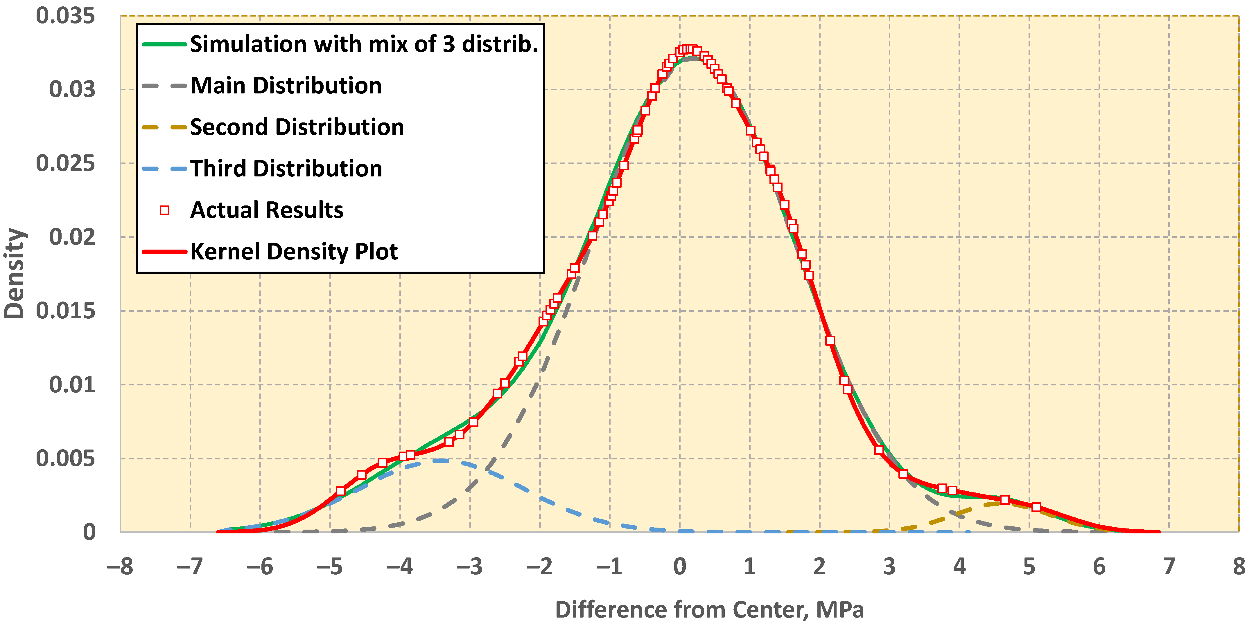
It creates a main normal distribution D₁ with mean value m₁ and standard deviation s₁ and two contaminating distributions D₂, D₃ with mean values m₂, m₃, and standard deviations s₂, s₃.

(ii)

The fractions of the contaminating distributions are fr₂ and fr₃, and, depending on these two values, the total distribution can be unimodal, bimodal, or trimodal.

(iii)

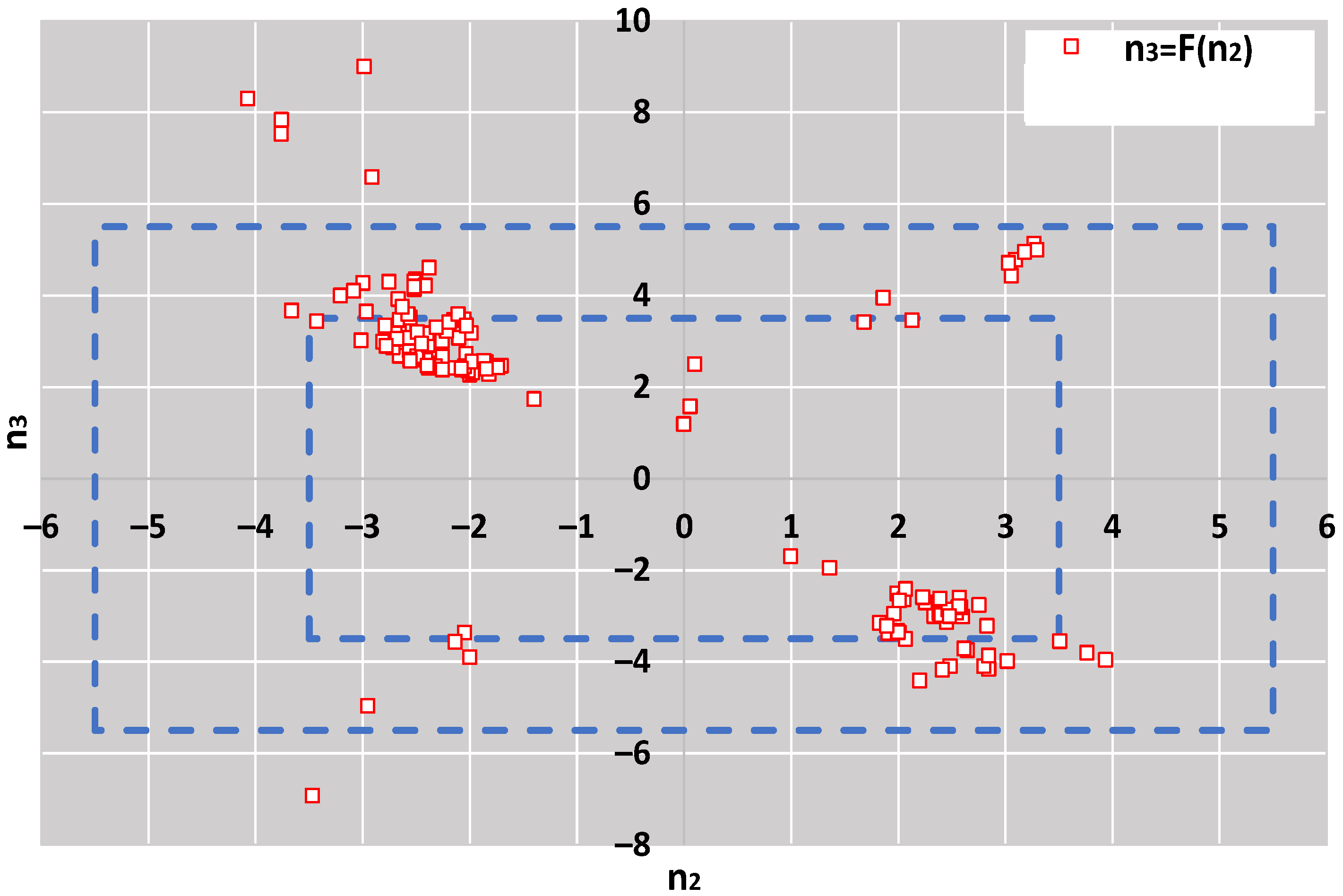
The mean values m₂ and m₃ differ by an integer number of standard deviations s₁ from m₁, n₂ and n₃, shown in Equation (3). In the case of trimodal distribution, if n₂·n₃ > 0, then D₂ and D₃ are both to the same side of the D₁. Otherwise, one is to the left and the other to the right of D₁.

$$m_2=m_1+n_2·s_1 , m_3=m_1+n_3·s_1 with \left|n_2\right|\le \left|n_3\right|, n_3\ge 0, and n_2\ge 0 or n_2<0$$

(3)

(iv)

According to the values of fr₂, fr₃, n₂, and n₃, the software calculates the values of Zu%, which are unsatisfactory compared to the normal distribution function with mean and standard deviation m₁ and s₁ correspondingly. These values are the initial values. For example, if m₁ = 0, s₁ = 2, s₂ = s₃ = 1, n₂ = −5, n₃ = 7, fr₂ = 0.05, and fr₃ = 0.05, then Zu% = 0.24 (from D₁) + 5.0 (from D₂) + 5.0 (from D₃) = 10.24.

(v)

The algorithm calculates all the estimators for the mean and standard deviation shown in Table 4 and the Zu% for the absolute values of the four Z-factors presented in the same table using a N_lab = 1000. For this number of participants, all estimators converge to their final value. As demonstrated in [24], N_lab = 400 is adequate for such convergence.

(vi)

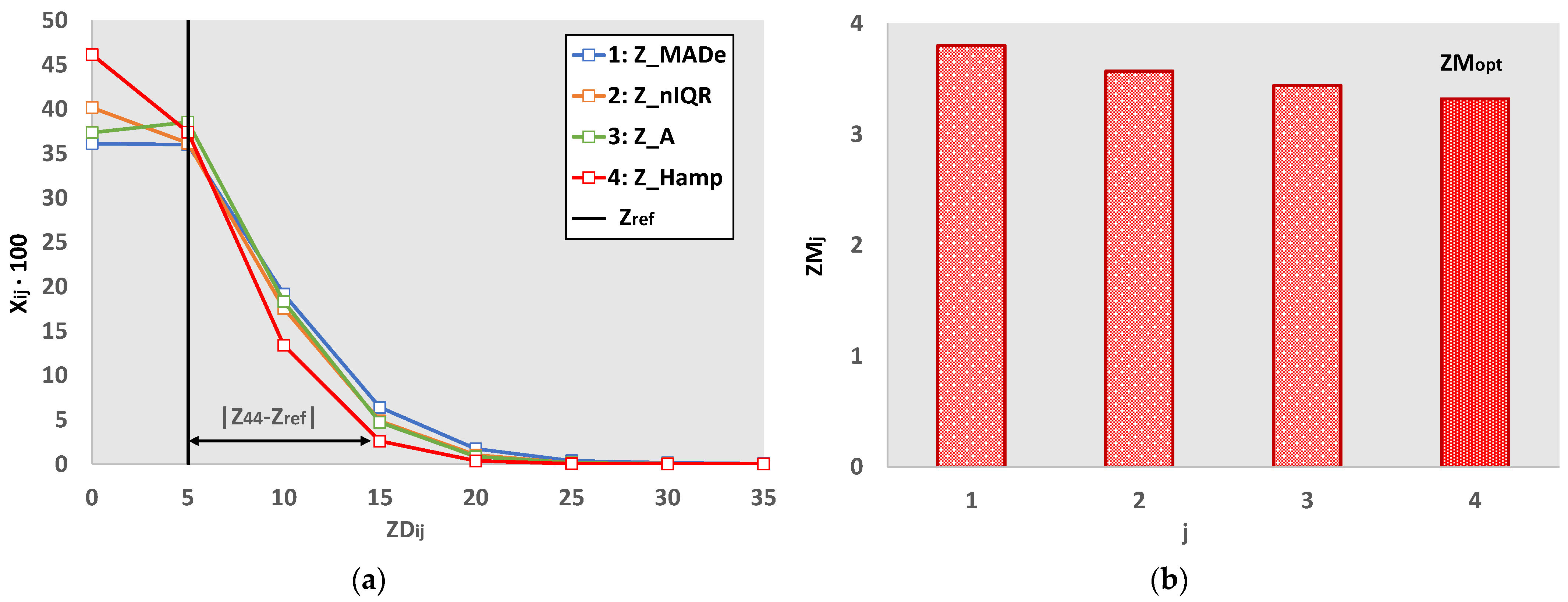
This previous study found that Z_MADe was the closest estimator of unacceptable Z-factors to the estimation based on the main normal distribution of step (iv). Its values corresponding to N_lab = 1000 represent the reference values, Z_ref.

(vii)

The simulations implemented all the settings shown in

Table 5. Simulation settings.

Setting	Value
Nlab	10, 15, 20, 30, 40, 60, 80, 100 and 1000 1
Nrep	2
sr	0.01
m1	100
s1	1, 2, 3, 4
m2	m2 = m1 + n2·s1, n2 = −8 to 8 and step 1
fr2	0, 0.05, 0.1, 0.15, 0.20 2
m3	m3 = m1 + n3·s1, n3 = 1 to 8 and step 1 3
fr3	0, 0.05, 0.1, 0.15
s2	1, 2, 3
s3	1, 2
Niter	1000
Ns	Up to 25 4
Nb	20 5

¹ If N_lab = 1000, then the N_s = 5. ² If fr₃ = 0, then the maximum value of fr₂ is 0.2. Otherwise fr_2Max = 0.15 and fr₂ + fr₃ ≤ 0.2. ³ If n₃ < 0, the distribution is symmetric about the Y-axis with that of n₃ > 0 and n₂ of opposite sign and the same absolute values. Therefore, the simulation results will be the same. ⁴ The algorithm stops earlier than 25 simulations if the new value of the average of each unacceptable Z-factor differs from the previous one by less than 0.1%. ⁵ If the number of distribution non-zero fractions is higher than 20, then N_b = 30 or 40.

for participants up to 100. The populations correspond to unimodal, bimodal, and trimodal distributions with a maximum total fraction of secondary distributions up to 0.2.

(viii)

For each mix of the three normal distributions, the software performs N_iter iterations and N_s simulations for each N_lab. Then it calculates the differential distribution of each of the four Zu% in at least twenty bins. The algorithm compares these results with the reference value using the distance of the distribution’s points from Z_ref provided by Equation (4). The Z-factor with the closest distance to the reference value is optimal.

$$Z{M}_j={\displaystyle \sum }_{i=1}^{Nmax}\left|Z{D}_{ij}-Z_{ref}\right|·X_{ij} , Z{M}_{opt}=\underset{}{\min }\left(Z{M}_j\right) for j=1 to 4$$

(4)

There are five components to this equation. ZM_j, X_ij, ZD_ij, Z_ref, and N_max. ZM_j denotes the mean of distances between the distribution of estimator j and Z_ref, X_ij is the fraction of the differential distribution at point i with a ZD_ij value on the X-axis, and N_max is the maximum i with a non-zero X_ij value. The best estimator is the one whose index j corresponds to ZM_j’s minimum. If the ZM value of another estimator differs by less than 1% from the minimum ZM, this also estimator is optimal. Figure 4 illustrates the above method of finding the most suitable estimator using the following model parameters. N_lab = 20; s₁ = 2; n₂ = −2; n₃ = 5; s₂ = 1; s₃ = 1; fr₂ = 0.1; fr₃ = 0.05.

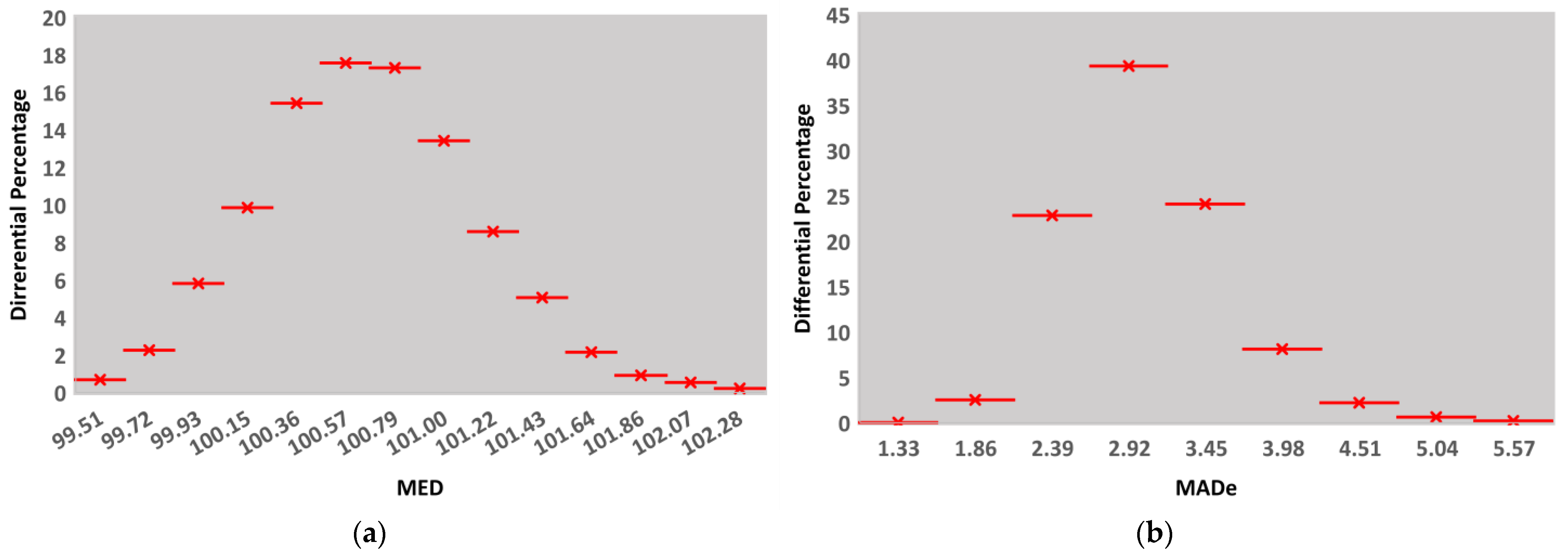
3.2. Initial Simulations

Monte Carlo simulation was first applied to study the distribution of the two statistics affecting the Z factors: the population’s mean and standard deviation. The algorithm created the frequency distributions of all the estimators in N_b bins, using the N_iter·N_s results of each statistic. These histograms, designed to investigate the symmetry of the distributions, are highly reliable because they incorporate up to 25,000 simulations. Figure 5 depicts such an example for MED and MADe. There is an asymmetry in both distributions, indicating that this skewness should be explored further. The skewness metric must be nonparametric because the approach used to detect outliers is. Additionally, all studied distributions are unimodal, sometimes with few frequency fractions over 0.01. In this study, we implement the simple formula provided by Groeneveld et al. [38] using the mean value, μ, and the median value, ν, of the distribution. The measure of dispersion in this formula, E(|X−ν|), is the mean value of the absolute differences between distribution values and the median. In this way, we avoid utilizing the more complicated formula described in many textbooks [39], involving the use of second and third-order moments. Equation (5) expresses the selected skewness measure, SK.

$$SK=\frac{\mu -\nu }{E\left(\left|X-\nu \right|\right)}$$

(5)

It is well known from very early research [40] that the nonparametric skewness always lies between −1 and +1. For symmetric distributions its value is zero. It is positive for right skewed distributions (μ > ν) and negative for left skewed distributions (μ < ν). For each robust statistic, the algorithm computes the mean value, μ, by summing the products of each differential fraction f_i, for I = 1 to N_b, with the average X_i of each interval of the histogram X-axis using Equation (6). The calculation of median value, ν, utilized linear interpolation between the points X_p, X_p+1, where f_p < = 0.5 and f_p+1 > = 0.5. Finally, Equation (7) provides the estimation E(|X−ν|).

$$\mu = {\displaystyle \sum }_{i=1}^{Nb}{X}_i·f_i$$

(6)

$$E\left(\left|X-\nu \right|\right)= {\displaystyle \sum }_{i=1}^{Nb}\left|X_i-\nu \right|·f_i$$

(7)

Figure 6 and Figure 7 present the SK values for various simulations: N_lab = 10, 20, 40, 80; s₁ = 2; n₃ = 7; n₂ = −7 to +7; s₂ = 1; s₃ = 1; fr₂ = 0.1; fr₃ = 0.05; from which one can conclude the following:

(i)

The distributions of mean are continuously positively skewed due to the assumption |n₂| < |n₃|. If n₃ =−7, and supposing the same condition between n₂, n₃, the distributions are symmetrical to the ones shown, but μ < ν and SK < 0.

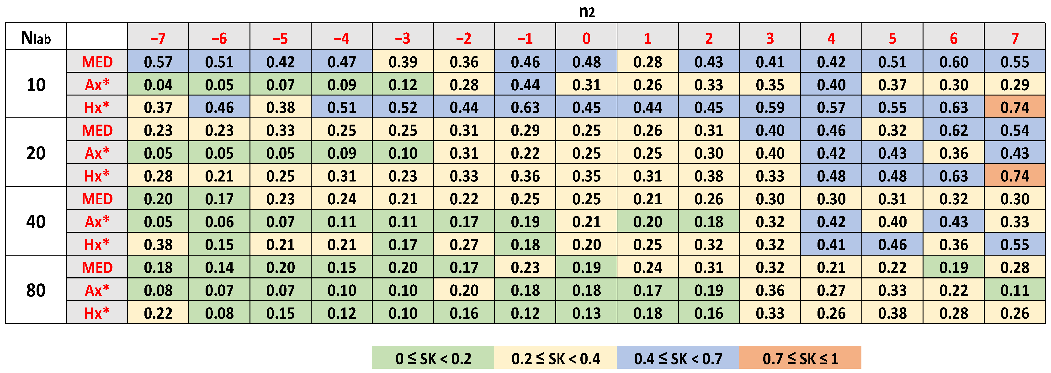
(ii)

We classified SK values into four regions: (a) 0 ≤ |SK| < 0.2; (b) 0.2 ≤ |SK| < 0.4; (c) 0.4 ≤ |SK| < 0.7; (d) 0.7 ≤ |SK| ≤ 1. As a rough guide, we can consider that if |SK| < 0.2, the departure from symmetry is low [41]. The skew is moderate for |SK| values in (b). The distribution is highly skewed for |SK| values in (c). Finally, the skew is very high for |SK| ≥ 0.7.

(iii)

The skewness of the estimators of mean increases, increasing n₂ from −7 to 7. For these estimators, the skewness decreases, increasing the number of participants. The distributions are highly symmetric for N_lab ≥ 40 and n₂ ≤ 0.

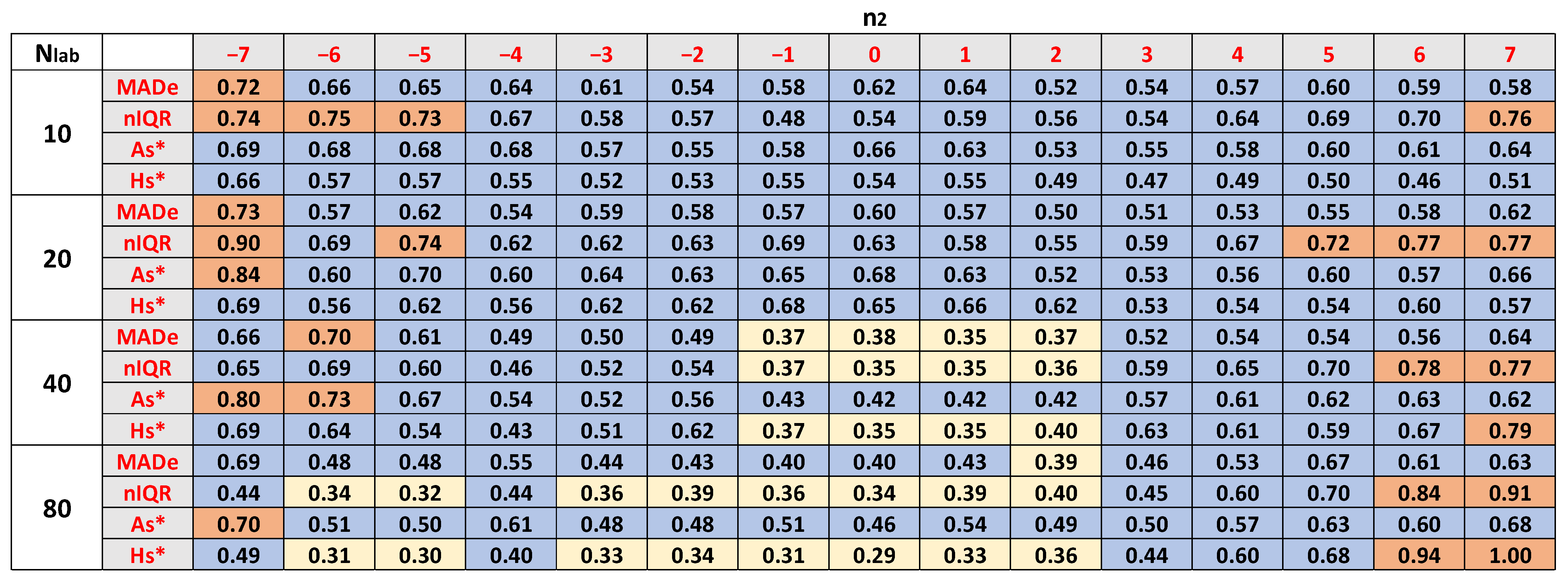
(iv)

The estimators of the mean have less skewness than those of standard deviation for the same N_lab and n₂. The best symmetry in the distributions of the latter occurs for N_lab ≥ 40 and n₂ between −1 and 1.

(v)

For low and high n₂ values, the skewness standard deviation sometimes becomes very high.

(vi)

The asymmetry of the two distributions indicates that the search for the best method regarding outliers should focus on their distribution for each performance statistic mentioned in Table 4.

4. Optimal Robust Estimators for Outlier Detection

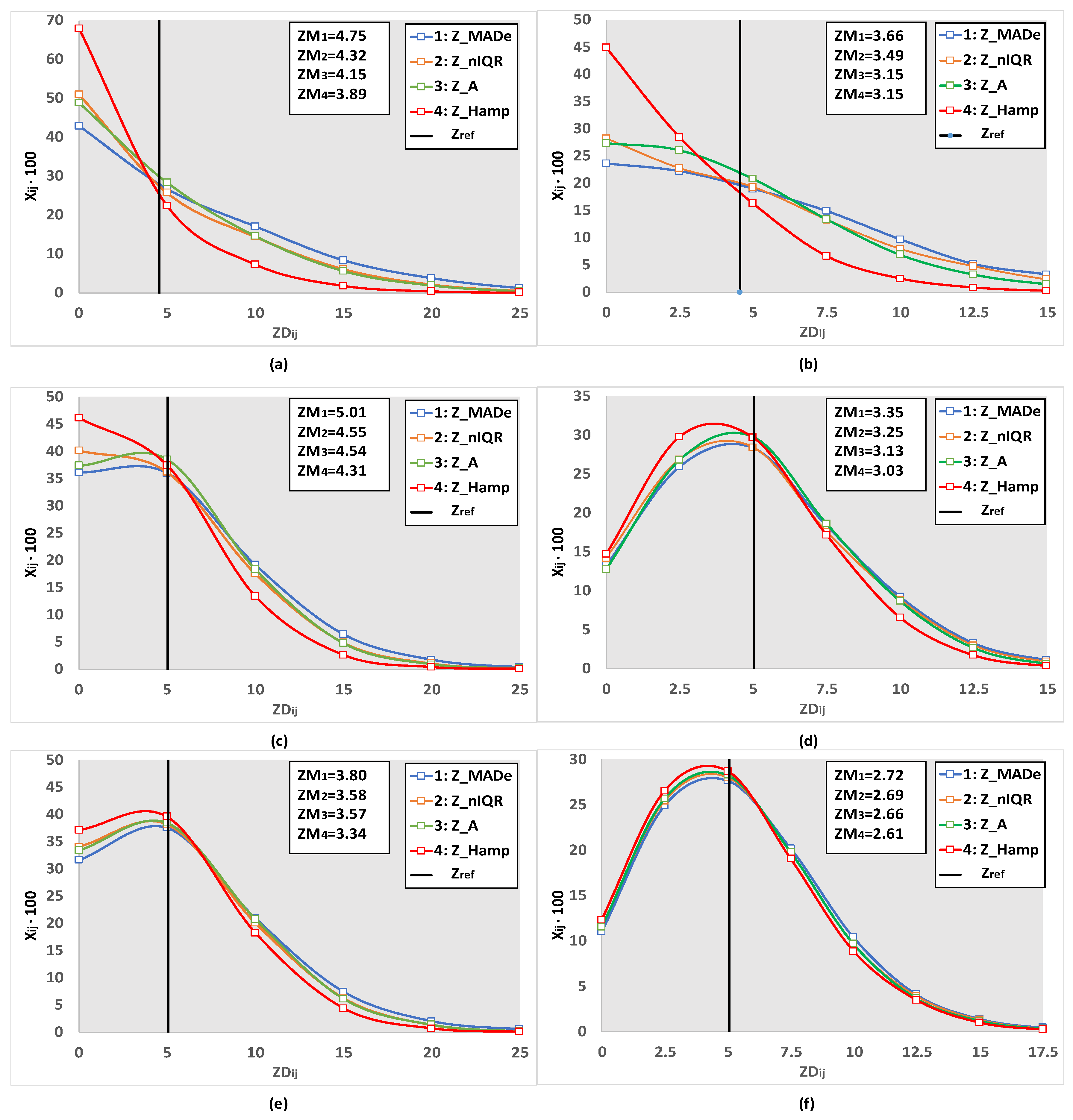
4.1. Shape of the Outliers Distribution

The distributions of outliers are not only skewed but sometimes not bell-shaped. Furthermore, they are discrete. For a certain number of participants, N_lab, each value ZD on the X-axis corresponds to an integer number of unsatisfactory results. For example, for N_lab = 40 and ZD = 5%, the outliers are 5/100·40 = 2. Figure 8 illustrates the above by implementing the four performance statistics in Table 4 and using six sets of model parameters.

Equation (4) defines the variables shown in Figure 8. The shape of the distribution of outliers strongly depends on the number of participants, the model parameters expressing the distribution of the results, and the performance statistic selected. All curves have a long right tail, but its thickness in each distribution depends on the performance estimator. In general, Z_Hamp shows thinner tails, thus a lower percentage of outliers significantly higher than the reference value, Z_ref. Figure 8 shows the mean distances ZM between each performance estimator and Z_ref. Z_Hamp is the most effective estimator for the examples presented. An intriguing case appears in Figure 8b: Z_Hamp and Z_A estimators are both optimal, despite their distinct distributions. It results from using the objective criterion of the mean distance of the distribution from Z_ref, which is particularly effective for strongly non-normal distributions.

4.2. Implementation of the Simulator

In the author’s experience, 10 to 100 labs participate in most PT schemes. Additionally, if the total contaminating population is more than 20% and very distant from the center, one of two things usually happens. (a) The samples are not homogenous enough, or (b) the labs use different measurement methods for the same analyte or property. ISO 13528:2015 dedicates a complete sub-section and an Annex to the first case [15]. The same standard suggests using a distinct assigned value for each measurement method for the second case [15]. As a result, the settings in Table 5 are of particular practical interest to those with expertise in PT schemes since they apply to most PT schemes with homogeneous test items, permitting one properly described measurement method per test.

The simulation implements Equation (4) to all the settings of Table 5 to find the best estimators for detecting outliers. The combination of s₁, s₂, and s₃ provides 4·3·2 = 24 triads. The simulation uses 12 out of 24, referred to as [s₁, s₂, s₃], where the three standard deviations are integers. For example [s₁, s₂, s₃] = 111 it means that s₁ = 1, s₂ = 1, and s₃ = 1. The set of applied [s₁, s₂, s₃] is as follows: 111, 211, 212, 222, 311, 321, 312, 322, 421, 412, 422, 432. The combination of fr₂ and fr₃ provides ten couples of [fr₂, fr₃], the following: [0, 0.05], [0, 0.10], [0, 0.15], [0, 0.20], [0.05, 0.05], [0.05, 0.10], [0.05, 0.15], [0.10, 0.05], [0.10, 0.10], [0.15, 0.05]. The simulator utilized all these combinations to obtain various unimodal, bimodal, and trimodal distributions. The maximum selected number of n₃, n_3MAX, depends on the value of s₁ as follows: (a) for s₁ = 1, 2, n_3MAX = 8; (b) for s₁ = 3, n_3MAX = 6; (c) for s₁ = 4, n_3MAX = 5.

Figure A1 and Figure A2 of Appendix A demonstrate two descriptive maps of optimal estimators for [s₁, s₂, s₃] = 222. The main conclusions from these results are the following:

(i)

For n₃ ≤ 3 and |n₂|< = 3, i.e., for relatively low differences between the mean values of contaminating and central distributions, Z_Hamp is almost always the best estimator.

(ii)

Considering all the combinations of [s₁, s₂, s₃] and [fr₂, fr₃], Z_Hamp is almost always the best in this range of n₂, n₃. Therefore, when at most half the distribution of each contaminating population is outside, left or right, of the central distribution, there is only one optimal estimator.

(iii)

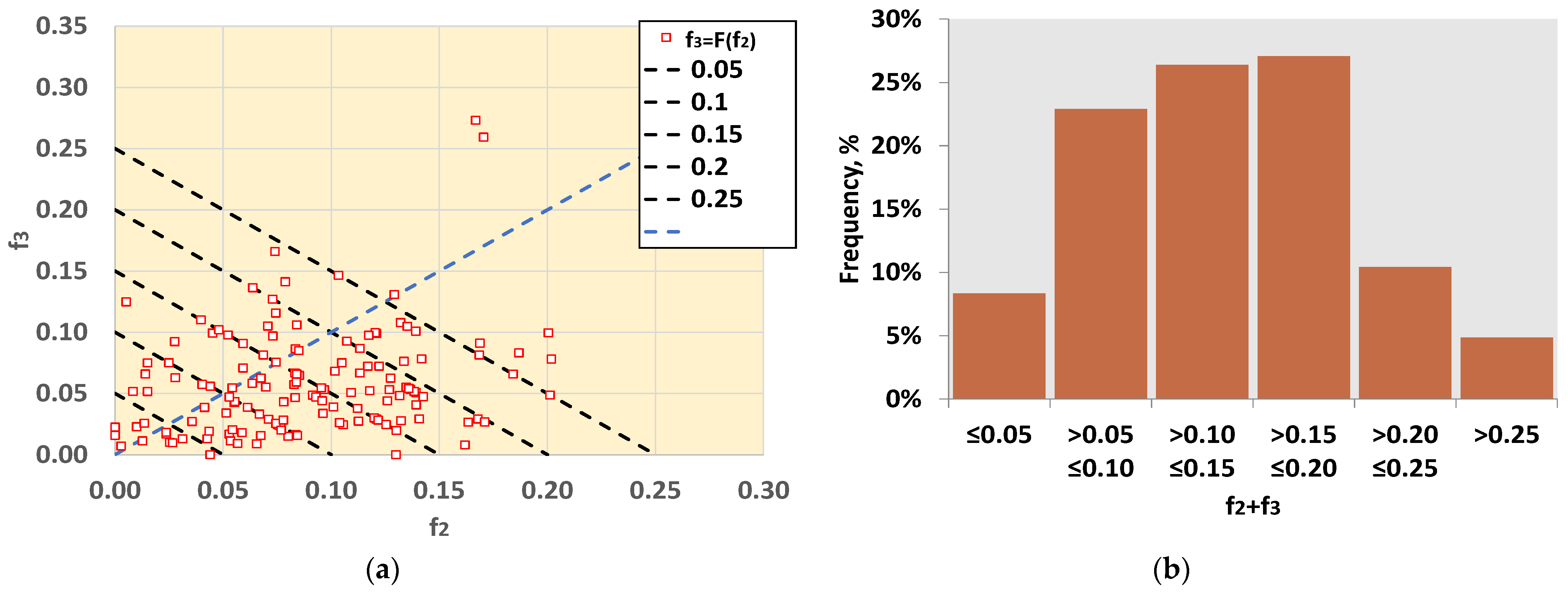
For higher values of n₃ and |n₂|, determining the most suitable estimator is a function of (a) the number of participants; (b) the distribution of the results, expressed by f₂, f₃, n₂, and n₃.

4.3. Simulation Results

The simulator calculates the results for all combinations [s₁, s₂, s₃] X [fr₂, fr₃], resulting in 120 matrices similar to those in Figure A1 and Figure A2, which are the exact solution of the optimization problem applying the criterion of Equation (4). Instead of this solution, we chose a functional sub-optimal one by grouping and classifying the parameters as follows:

(i)

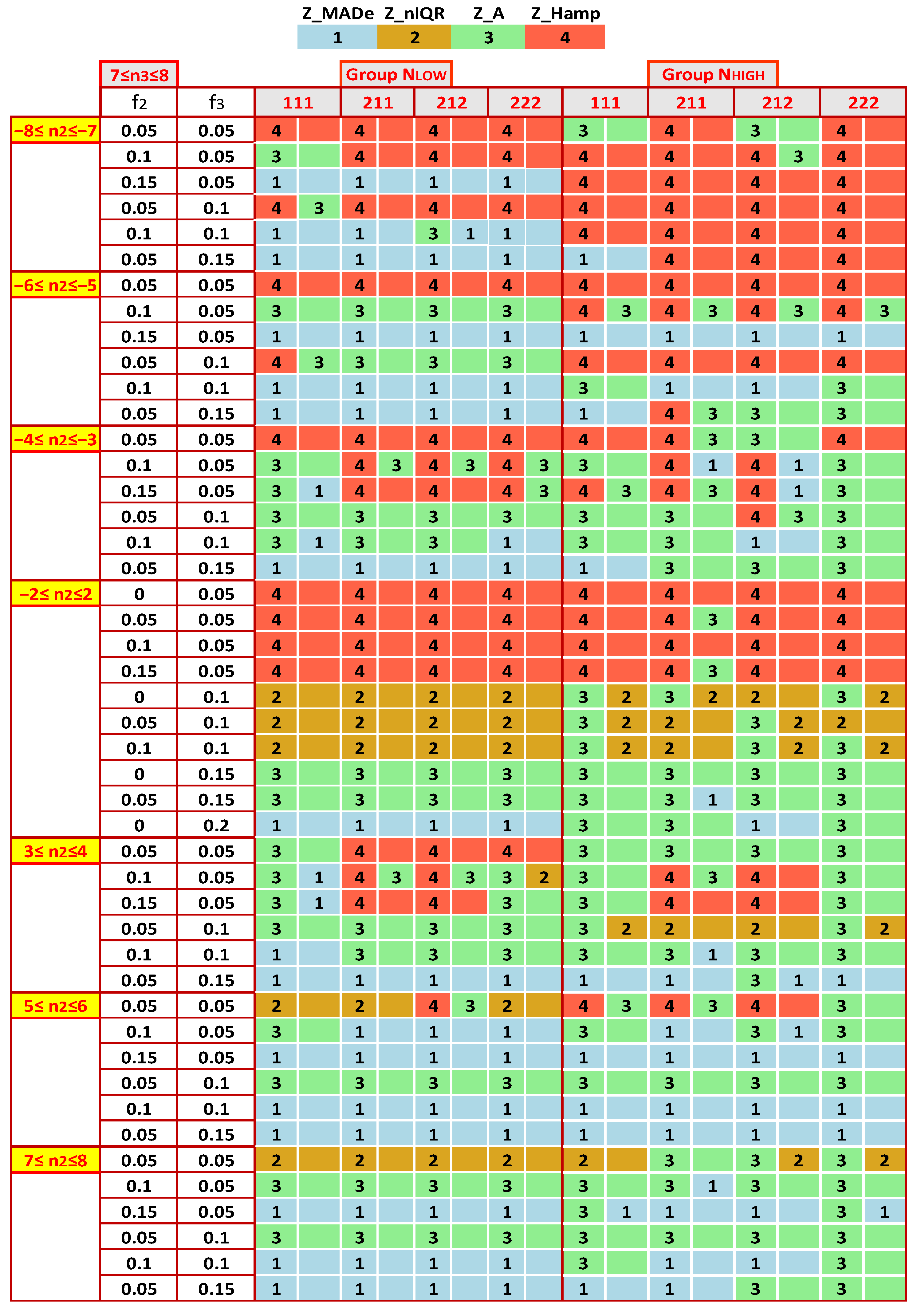
The algorithm initially generates two groups: (a) a small population of participants, N_LOW, with N_lab = 10, 15, 20, and 30; (b) a large one, N_HIGH, with N_lab = 40, 60, 80, and 100.

(ii)

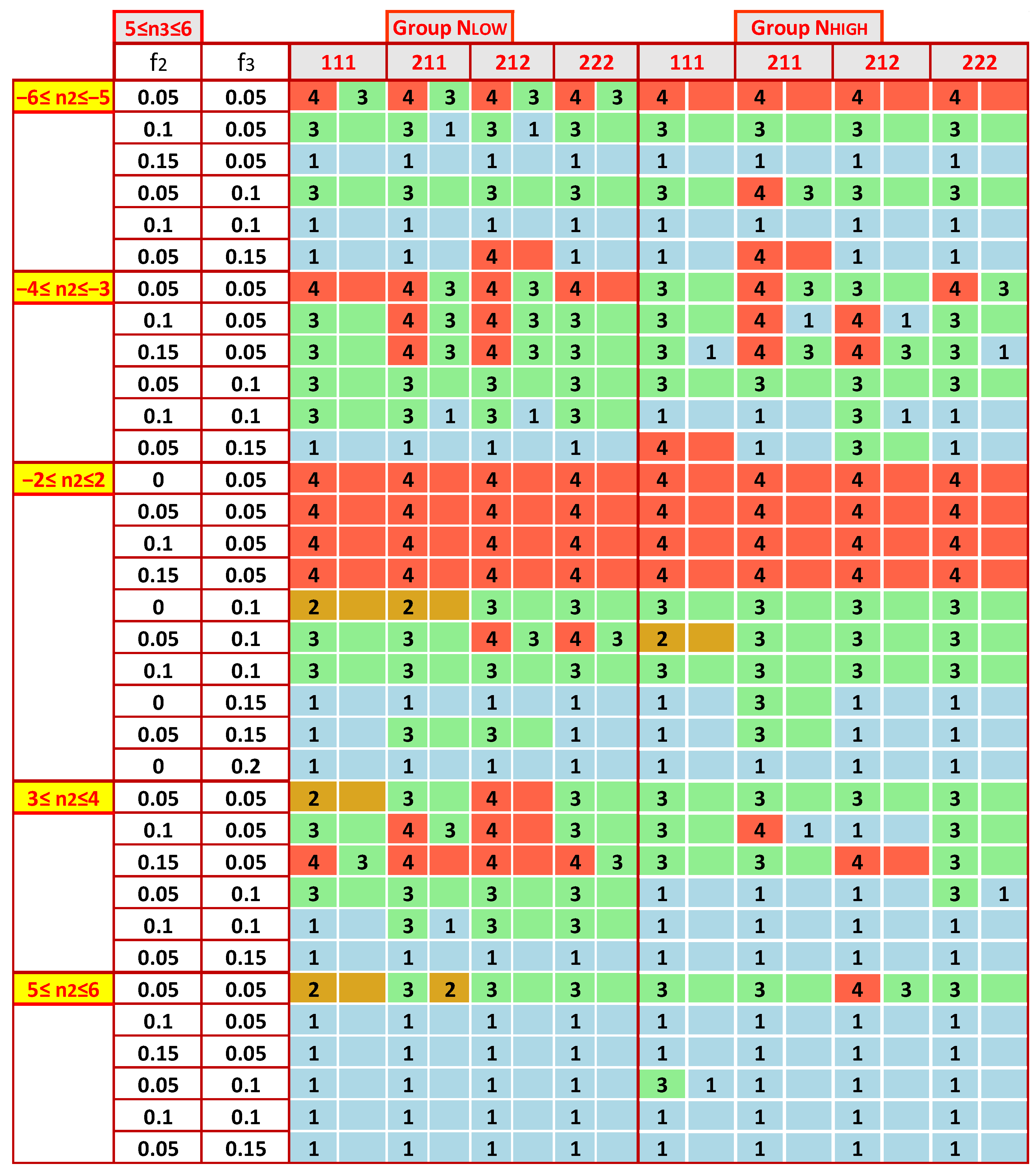
It then creates at most seven regions of n₂ by keeping|n₂| < n₃, the following: (a) −7 ≤ n₂ ≤ −8; (b) −6 ≤ n₂ ≤ −5; (c) −4 ≤ n₂ ≤ −3; (d) −2 ≤ n₂ ≤ 2 (e) 3 ≤ n₂ ≤ 4 (f) 5 ≤ n₂ ≤ 6 (g) 7 ≤ n₂ ≤8. It is seven regions when n_3MAX is 8, but five when n_3MAX is less.

(iii)

Afterwards, it counts the occurrences of each estimator as optimal in each region and calculates their percentages.

(iv)

An optimal estimator is the one with the highest percentage and those whose percent of appearance differs by up to 10% from the maximum.

(v)

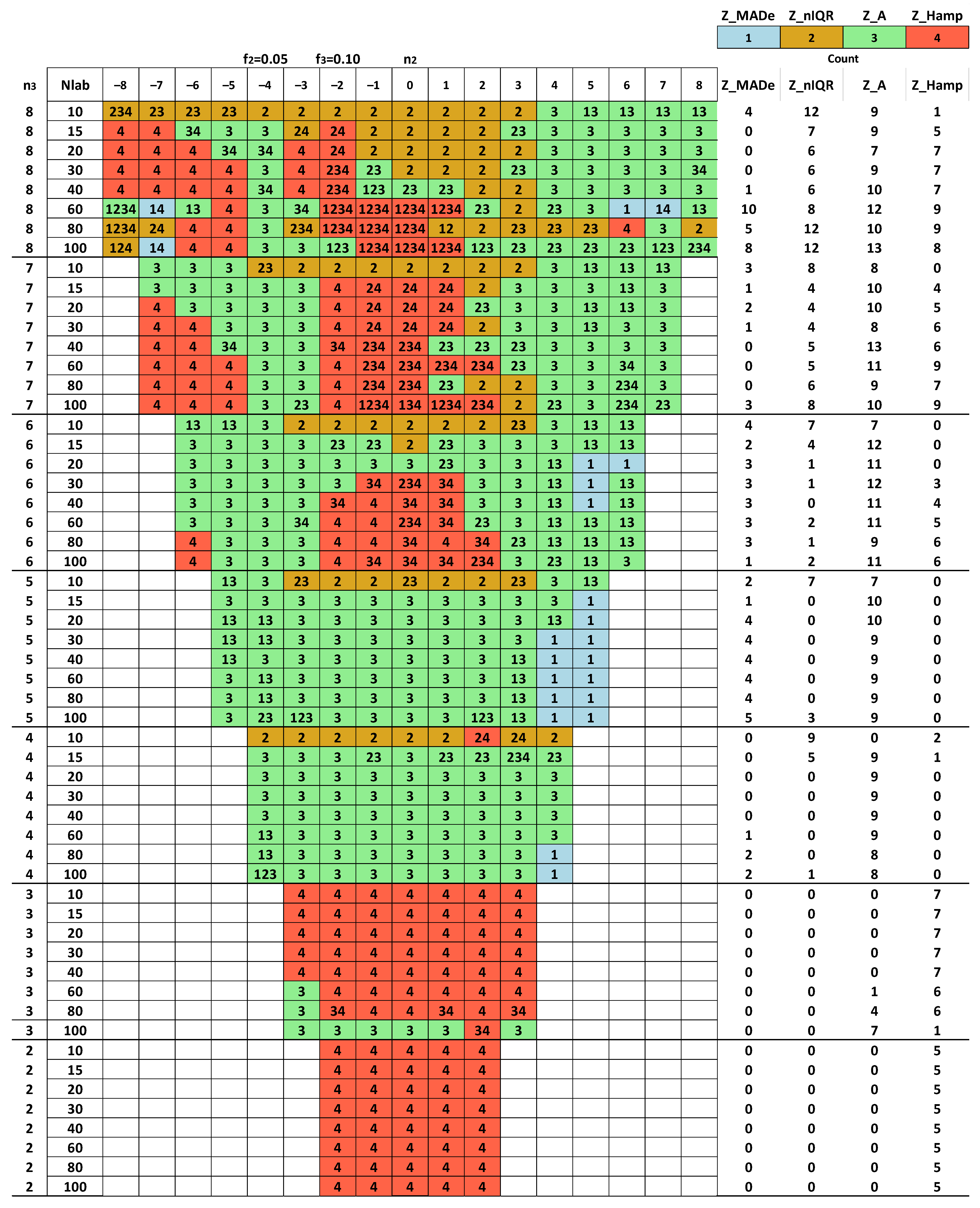
Next is the creation of tables with the results per n₃ and [s₁, s₂, s₃].

Figure 9, Figure 10 and Figure 11 show the most accurate estimators for [s₁, s₂, s₃] = 111, 211, 212, 222 and 7 ≤ n₃ ≤ 8, 5 ≤ n₃ ≤ 6, n₃ = 4. Appendix B contains all the remaining results for s₁ = 3 and 4. We do not show the results for n₃ = 2,3 since Z_Hampel is always much superior to the second estimator, i.e., Z_Hampel is the best. Figure 9 shows that the four estimators are numbered and colored. Two columns are present for each [s₁, s₂, s₃] because two optimal estimators exist for some parameter sets.

The main conclusions derived from the five results maps of Figure 9, Figure 10, Figure 11, Figure A3 and Figure A4 are as follows:

(i)

For n₃ > 3 and |n₂| > 3, determining the optimal estimator depends on (a) the number of participants; (b) the distribution of the results, expressed by the model parameters, verifying absolutely the conclusion derived from the examples in Figure A1 and Figure A2.

(ii)

For the same n₃, the distribution of the most accurate performance statistics as a function of n₂ is not symmetrical around the center. For all n₃, the estimators for −8 ≤ n₂ ≤ −7 and −6 ≤ n₂ ≤ −5 differ significantly from the ones for 7 ≤ n₂ ≤ 8 and 5 ≤ n₂ ≤ 6. More symmetrical patterns appear in zones −4 ≤ n₂ ≤ −3 and 3 ≤ n₂ ≤ 4.

(iii)

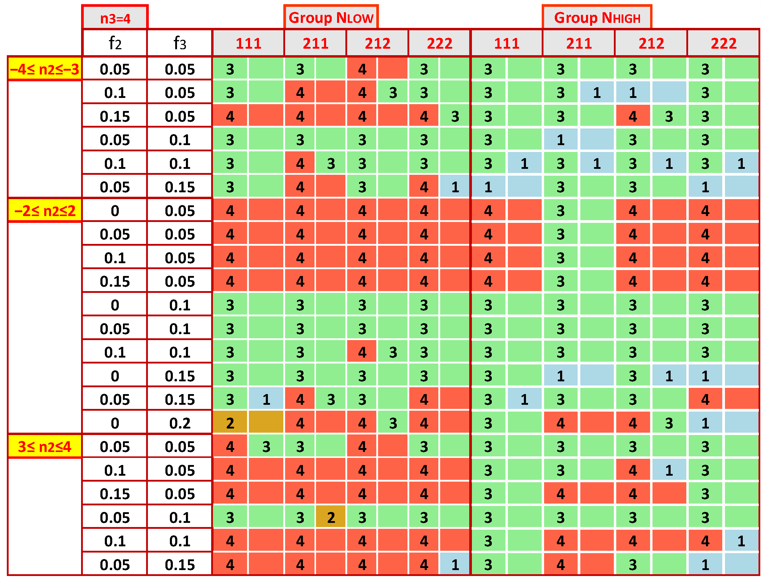
With the same model parameters, the results are similar for the two groups N_LOW and N_HIGH, but not in all cases. For example, for 7 ≤ n₃ ≤ 8 and −7 ≤ n₂ ≤ −8, Z_Hampel appears as the optimal performance statistic much more in the N_HIGH group than in N_LOW. In contrast, this estimator is found significantly more frequently in the low number of labs than in N_HIGH when n₃ = 4.

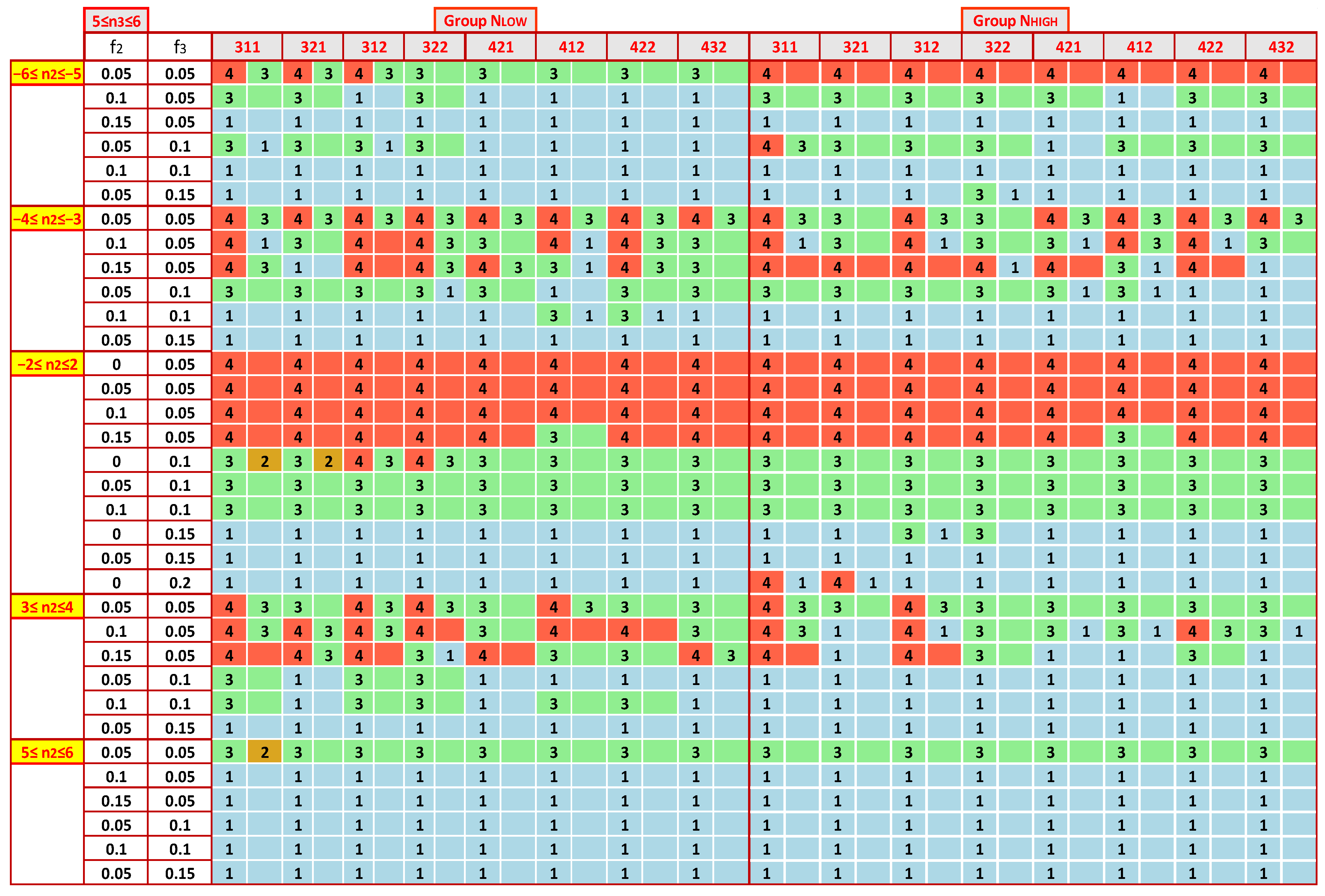
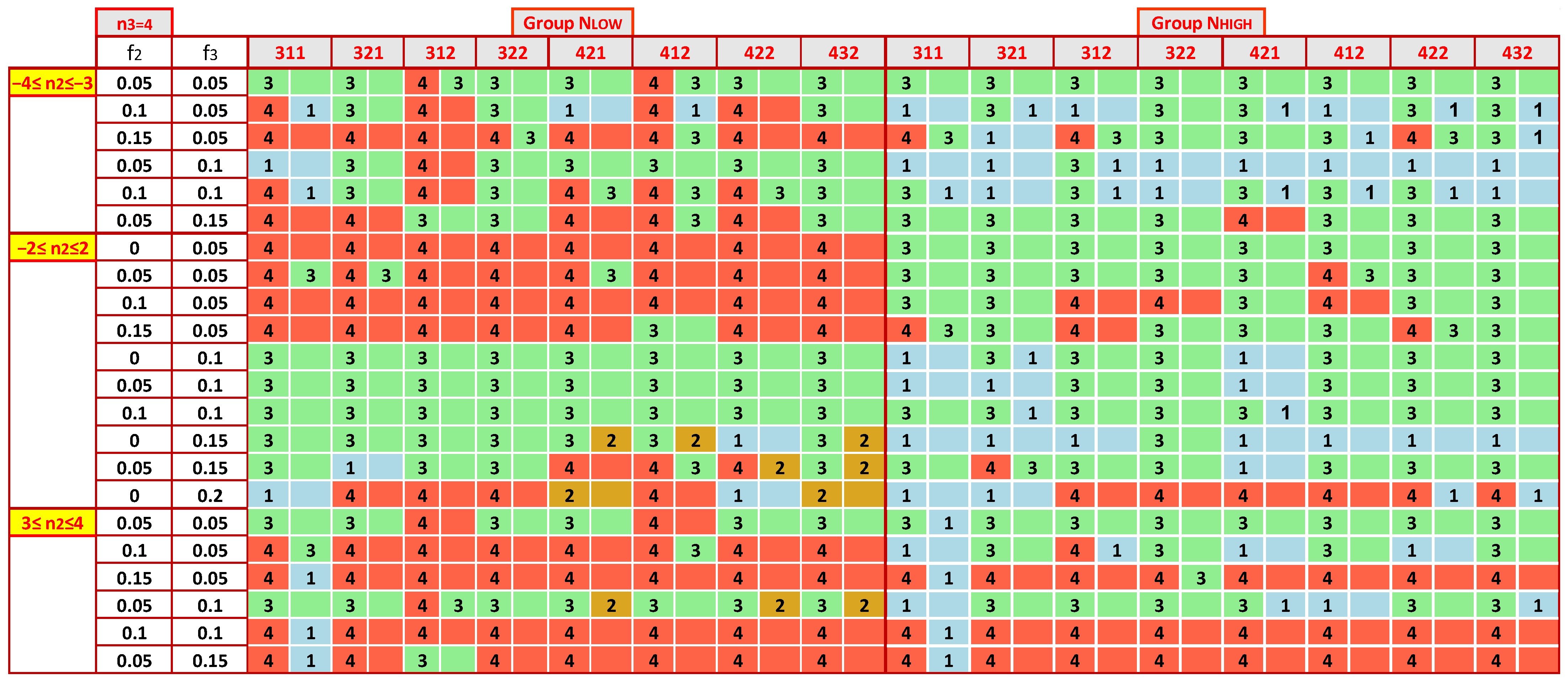
(iv)

The selection of the most appropriate estimator is not so sensitive to the choice of the mixture of standard deviations, [s₁, s₂, s₃]. When comparing Figure 10, Figure 11, Figure A3 and Figure A4, one finds that in enough cases, the optimal statistic is the same for the same group of labs, n₃, n₂, f₂, and f₃, concluding that the impact of [s₁, s₂, s₃] is less strong than that of the other parameters.

(v)

With a contaminating population fraction f₃ of 0.05 and distribution diverging relatively little from the bimodal with −2 ≤ n₂ ≤ 2, the Z_Hamp is most often found. However, this rule is not absolute. Figure A4 demonstrates that for the group N_HIGH, n₃ = 4, and s₁ = 3 or 4, Z_A is the most suitable.

(vi)

In some cases, there are expanded zones where one estimator outperforms the others, increasing the robustness of the suggested solution. For example, in Figure 10 and Figure A3, for 5 ≤ n₂ ≤ 6, the first choice is the Z_MADe. In Figure 10, Figure 11, Figure A3 and Figure A4, for −2 ≤ n₂ ≤ 2 and f₃ = 0.10 the correct selection is Z_A.

(vii)

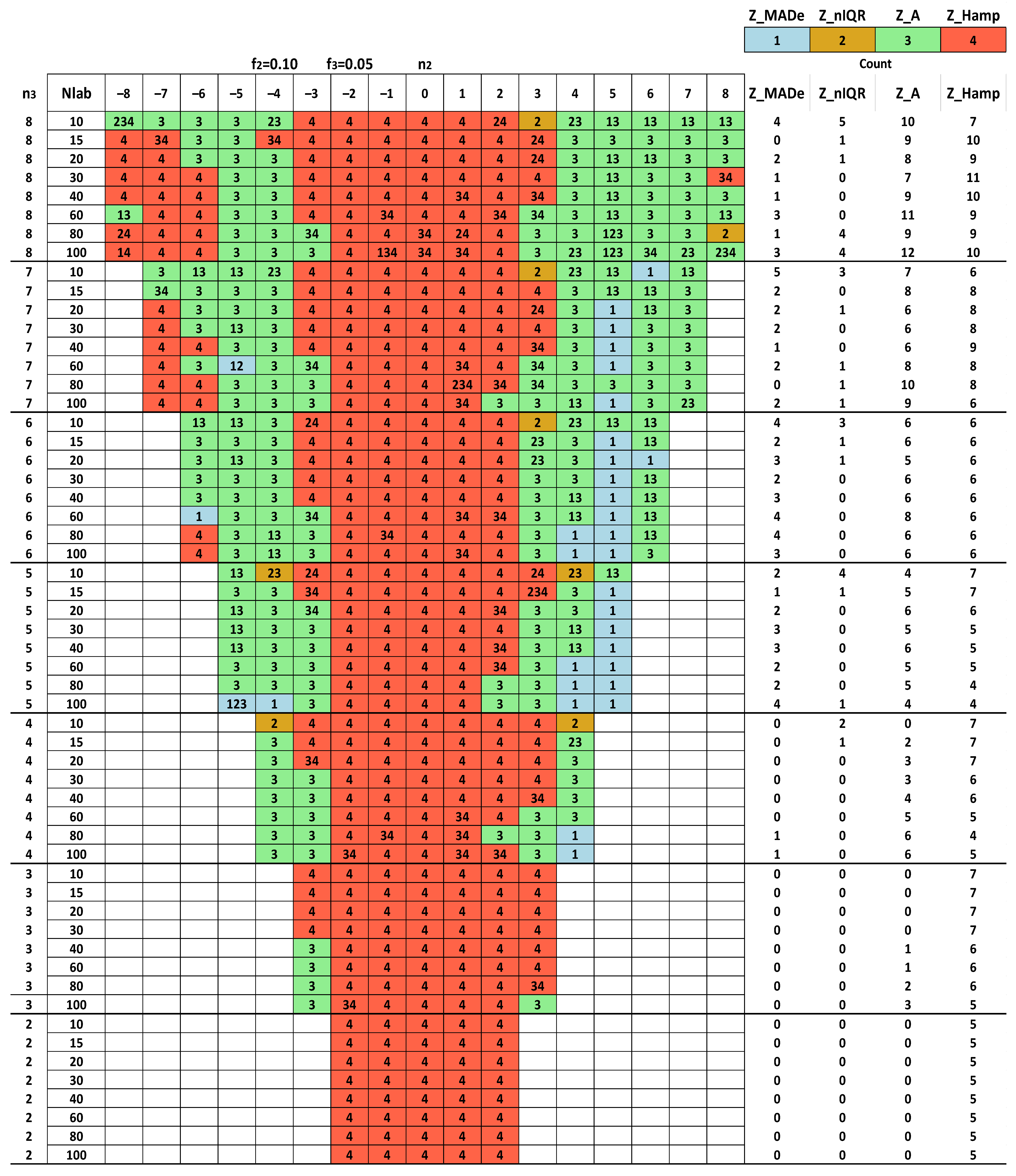
For N_LOW and N_HIGH groups, Figure 12 illustrates a rough tendency for the preferred statistics as a function of the zones of n₂, n₃, and f₃. For each region, the algorithm counts the occurrences of each estimator in the maps depicted in Figure 9, Figure 10, Figure 11, Figure A3 and Figure A4. It calculates their percentages and considers as optimal statistics those that are up to 10% below the maximum.

(viii)

The results of Figure 12 are only a rough guide to choosing the most appropriate estimator, demonstrating that there is no unique solution, and the best selection depends on the data distribution.

Although a machine learning technique, like the Support Vector Machine [42], could better classify the data, the presented solution is directly applicable. The PT schemes can apply the following procedure to implement the presented technique of finding the most appropriate robust estimator. Following verification of the homogeneity of the test items and the use of the same method of analysis per test, the PT expert should build the kernel density plot, enabling him to find the optimal mix of at most three Gaussian approximating this plot. If the PT scheme organizer executes the test several times a year, selecting the results of the latest and several recent rounds to generate kernel plots is preferable. The latest data have a significant probability of belonging to a population similar to the recent results population, especially if the same or almost the same laboratories participate. However, if PT scheme experts used only the last round to build the distribution, the parameters could have severe uncertainty, especially if N_lab is small. The next step is to normalize the parameters of the found normal distributions based on the mean value of the central one using Equation (8).

$$m_i=\frac{m_{i, Act}}{m_{1, Act}}·100 s_i=\frac{s_{i, Act}}{m_{1, Act}}·100 i=1, 2, 3$$

(8)

The symbols m_i,Act and s_i,Act, for I = 1,2,3, denote the mean value and the standard deviation of the three normal distributions simulating the kernel density plot. The parameters fr₁, fr₂, fr₃, and n₂, n₃ in Table 1 are independent of normalization.

Rounding the algebraic distances n₂, n₃, and the three standard deviations to the nearest integer follows. The same is done with the fractions fr₂ and fr₃ to the nearest multiple of 0.05. Next is to check if all the parameters are within the ranges given in Figure 9, Figure 10, Figure 11, Figure A3 and Figure A4. If n₃ < 0, and |n₃| > |n₂|, the symmetrical case by changing the signs of n₂ and n₃ provides the same optimal estimator. If this check is positive, the choice is the estimator that the Figures demonstrate. If f₂ + f₃ ≥ 0.25 but |n₂| ≤ 3 and |n₃| ≤ 3, Z_Hamp is the most appropriate selection, as already shown in 4.2. Otherwise, the figures are not applicable to such a high percentage of contaminating populations. The same happens if |n₃| > n_3MAX, as provided in Section 4.2.

The 144 kernel density plots analyzed in Section 2 represent a sufficiently large sample to apply the simulation results of the mentioned five figures to the actual conditions of a PT scheme operating systematically for years. Figure 2 and Figure 3 summarize the model parameters found. In case some real [s₁, s₂, s₃] sets are not present in the simulation results, we selected from the figures those [s₁, s₂, s₃] that are closest to the actual ones. The group chosen is always the N_LOW, as 11–14 labs participate in each test.

Table 6. Percentages of estimators for each |n₃| region and for all sets.

	Percentages
Estimator	|n3| ≤ 3	4 ≤ |n3| ≤ 5	|n3| ≥ 6	All n3
Z_MADe	0	2.5	0	0.7
Z_nIQR	0	0	0	0
Z_A	0	30	0	8.3
Z_Hamp	100	55	66.7	86.1
Not Applicable	0	12.5	33.3	4.9
Percentage of each |n3| region	68	27.8	4.2	100

summarizes the best estimators for detecting outliers for model parameters computed from actual and multiple tests.

The low population of results with |n₃| ≥ 6 shows that participants try to improve their performance and the PT scheme is well organized and mature. Only in 4.9% out of the 144 cases the parameters of the kernel density plots are outside the studied range. Z_Hampel significantly outperforms the other estimators when applied to multiple distributions of the results of a well-performing PT scheme. The conclusion is not general, but one can assume that in continuous and mature PT schemes with a limited number of participants, the Z_Hampel estimator is the suitable choice.

5. Conclusions

This study investigated the robust estimators of PT schemes in outlier detection, listed in ISO 13528:2015, using tools developed in [24] and analyzing the distribution of unsatisfactory results with |Z| > 3. The approach combines various techniques and criteria: (a) robust estimators of the population mean and dispersion; (b) kernel density plots; (c) distributions derived from the mix of at most three Gaussians; (d) Monte Carlo simulations; (e) Z-factors.

One portion of the algorithm created kernel density plots for 144 datasets of cement’s chemical, physical, and mechanical properties, belonging to a continuous PT scheme of cement. It approximated each KDP by summing suitable fractions of the Gaussians, which have adjustable parameters. The fit is sufficiently efficient for all the sets, with a coefficient of determination of 0.9917 ± 0.0051. While the central distribution is the primary one, the others contaminate it. The fractions of the three Gaussians, their standard deviations, and the algebraic distance of the mean of the contaminating ones from the center define the shape of the results’ kernel density plot. The distribution of these variables determined the minimum range of the simulation’s parameters.

Assuming a distribution of a large number of results containing Zu% unsatisfactory results according to EN ISO/IEC 17043:2010, the simulator can find the best estimators. For each PT round, the simulator considers a wide range of parameters and takes into account between 10 and 100 participants. The fraction of the two contaminating Gaussians is up to 0.20 of the total. The model was applied to study the distribution of the mean and the standard deviation of the population. We found that both are unimodal but skewed. For the standard deviation, the skewness ranges from moderate to very high. The distributions of outliers are not only skewed but sometimes not bell-shaped. The metric to find the best robust estimator must be nonparametric because the approach used to detect unsatisfactory results is. The software calculates the differential distribution of each estimator and compares these results with the reference value using the distance of the distribution’s points from Z_ref. The estimator with the minimum value is the best.

The simulator calculates the optimal statistics for all combinations, resulting in 120 matrices of results. Instead of this solution, we chose a functional sub-optimal one by grouping and classifying the model parameters according to the number of participants, the distance of the secondary distributions from the central one, and the standard deviation of the Gaussians. In each region, the estimators appearing most often are the best. Whenever at most half of the distribution of each contaminating population is outside the central distribution, the Z_Hamp estimator is the most suitable. For all other cases, we concluded with five result tables, which form a building block of this study and a robust tool for choosing the most accurate statistic. Z_Hamp is most frequently found for distributions that diverge relatively little from the bimodal, and the fraction of the most distant population from the center is 0.05.

We applied the suggested method to the referred 144 datasets of a continuous PT scheme for cement. We used their kernel density plots and the parameters of the Gaussian populations to approximate them. The parameters of the KDPs fall outside the studied range only in 4.9% of these data. Z_Hampel is the most suitable estimator in 86.1% of this population of results derived from a stably performing PT scheme.

In the author’s experience, 10 to 100 labs participate in most PT schemes, so the results presented are of fairly general application. One can use the reference values derived from Z_MADe when there are more participants. After ensuring that the same method of analysis is used per test and verifying the homogeneity of the samples, the technical expert of a PT can apply the estimators generated by the sub-optimal solution. It is first necessary to build the kernel density plot per test and round, or over the recent rounds if the participants are limited, and then to adjust the parameters of the three Gaussian. If these are within the range presented in this study, then the estimator given in the corresponding Figure is most likely the best one.

Based on the above arguments, the novelty of this study is the generalized assessment of the effectiveness of the robust statistics listed in 13528:2015 in detecting outliers. We generated tables of optimal estimators for a wide range of participants and distributions of results, especially useful for existing and new PT schemes. The proposed method applies to 95.1% of the results for an existing PT for cement. The data cover nine years. The investigation of the best estimators can continue in the following two directions:

▪

direct use of the kernel density plots in determining the best statistic

▪

estimators’ comparisons for Z-factors of absolute value between two and three.

Furthermore, ISO 13528:2015 in Section C.6 states that the PT provider may use other robust estimators, subject to demonstrating their efficiency in fulfilling the particular requirements of the PT scheme. The simulation developed and the rich dataset of PT results used in this study could assist in investigating and comparing the effectiveness of regression or multivariate models when applied to PT schemes.

References

1. EN ISO/IEC 17043:2010; Conformity Assessment—General Requirements for Proficiency Testing. CEN Management Centre: Brussels, Belgium, 1994; pp. 2–3, 8–9,30–33.
2. Hampel, F.R.; Ronchetti, E.M.; Peter, J.; Rousseeuw, P.J.; Stahel, W.A. Robust Statistics: The Approach Based on Influence Functions; John Wiley & Sons, Inc.: New York, NY, USA, 1986. [Google Scholar]
3. Huber, P.J.; Ronchetti, E.M. Robust Statistics, 2nd ed.; John Wiley & Sons, Inc.: Hoboken, NJ, USA, 2009. [Google Scholar]
4. Wilcox, R. Introduction to Robust Estimation and Hypothesis Testing, 3rd ed.; Elsevier, Inc.: Waltham, MA, USA, 2013. [Google Scholar]
5. Maronna, R.A.; Martin, R.D.; Yohai, V.J.; Salibián-Barrera, M. Robust Statistics: Theory and Methods (with R), 2nd ed.; John Wiley & Sons, Inc.: Hoboken, NJ, USA, 2018. [Google Scholar]
6. Hund, E.; Massart, D.L.; Smeyers-Verbeke, J. Inter-laboratory Studies in Analytical Chemistry. Anal. Chim. Acta 2000, 424, 145–165. [Google Scholar] [CrossRef]
7. Daszykowski, M.; Kaczmarek, K.; Vander Heyden, Y.; Walczaka, B. Robust statistics in data analysis—A review: Basic concepts. Chemom. Intell. Lab. Syst. 2007, 85, 203–219. [Google Scholar] [CrossRef]
8. Shevlyakov, G. Highly Efficient Robust and Stable M-Estimates of Location. Mathematics 2021, 9, 105. [Google Scholar] [CrossRef]
9. Ghosh, I.; Fleming, K. On the Robustness and Sensitivity of Several Nonparametric Estimators via the Influence Curve Measure: A Brief Study. Mathematics 2022, 10, 3100. [Google Scholar] [CrossRef]
10. Zimek, A.; Filzmoser, P. There and back again: Outlier detection between statistical reasoning and data mining algorithms. WIREs Data Min. Knowl. Discov. 2018, 8, e1280. [Google Scholar] [CrossRef] [Green Version]
11. Roelant, E.; Van Aelst, S.; Willems, G. The minimum weighted covariance determinant estimator. Metrika 2009, 70, 177–204. [Google Scholar] [CrossRef]
12. Cerioli, A. Multivariate outlier detection with high-breakdown estimators. J. Am. Stat. Assoc. 2010, 105, 147–156. [Google Scholar] [CrossRef]
13. Rousseeuw, P.J.; Leroy, A.M. Robust Regression and Outlier Detection; John Wiley & Sons, Inc.: New York, NY, USA, 1987. [Google Scholar]
14. Kalina, J.; Tichavský, J. On Robust Esti ation of Error Variance in (Highly) Robust Regression. Meas. Sci. Rev. 2020, 20, 6–14. [Google Scholar] [CrossRef] [Green Version]
15. ISO 13528:2015; Statistical Methods for Use in Proficiency Testing by Interlaboratory Comparison. 2nd ed, ISO: Geneva, Switzerland, 2015; pp. 10–12, 32–33,44–51, 52–62.
16. ISO 5725-2:1994; Accuracy (Trueness and Precision) of Measurement Methods and Results—Part 2: Basic Method for the Determination of Repeatability and Reproducibility of a Standard Measurement Method. 1st ed. ISO: Geneva, Switzerland, 1994; pp. 10–14, 21–22.
17. ISO 5725-5:1998; Accuracy (Trueness and Precision) of Measurement Methods and Results—Part 5: Alternative Methods for the Determination of the Precision of a Standard Measurement Method. 1st ed. ISO: Geneva, Switzerland, 1998; pp. 35–36.
18. Rosário, P.; Martínez, J.L.; Silván, J.M. Evaluation of Proficiency Test Data by Different Statistical Methods Comparison. In Proceedings of the First International Proficiency Testing Conference, Sinaia, Romania, 11–13 October 2007. [Google Scholar]
19. Srnková, J.; Zbíral, J. Comparison of different approaches to the statistical evaluation of proficiency tests. Accredit. Qual. Assur. 2009, 14, 373–378. [Google Scholar] [CrossRef]
20. Tripathy, S.S.; Saxena, R.K.; Gupta, P.K. Comparison of Statistical Methods for Outlier Detection in Proficiency Testing Data on Analysis of Lead in Aqueous Solution. Am. J. Theor. Appl. Stat. 2013, 2, 233–242. [Google Scholar] [CrossRef]
21. Skrzypczak, I.; Lesniak, A.; Ochab, P.; Górka, M.; Kokoszka, W.; Sikora, A. Interlaboratory Comparative Tests in Ready-Mixed Concrete Quality Assessment. Materials 2021, 14, 3475. [Google Scholar] [CrossRef]
22. De Oliveira, C.C.; Tiglea, P.; Olivieri, J.C.; Carvalho, M.; Buzzo, M.L.; Sakuma, A.M.; Duran, M.C.; Caruso, M.; Granato, D. Comparison of Different Statistical Approaches Used to Evaluate the Performance of Participants in a Proficiency Testing Program. Available online: https://www.researchgate.net/publication/290293736_Comparison_of_different_statistical_approaches_used_to_evaluate_the_performance_of_participants_in_a_proficiency_testing_program (accessed on 2 November 2022).
23. Kojima, I.; Kakita, K. Comparative Study of Robustness of Statistical Methods for Laboratory Proficiency Testing. Anal. Sci. 2014, 30, 1165–1168. [Google Scholar] [CrossRef] [PubMed] [Green Version]
24. Tsamatsoulis, D. Comparing the Robustness of Statistical Estimators of Proficiency Testing Schemes for a Limited Number of Participants. Computation 2022, 10, 44. [Google Scholar] [CrossRef]
25. Yohai, V. High Break-Down Point and High Efficiency Robust Estimates for Regression. Ann. Stat. 1987, 15, 642–656. [Google Scholar] [CrossRef]
26. Gervini, D.; Yohai, V. A Class of Robust and Fully Efficient Regression Estimators. Ann. Stat. 2002, 30, 583–616. [Google Scholar] [CrossRef]
27. Pitselis, G. A Review on Robust Estimators Applied to Regression Credibility. J. Comput. Appl. Math. 2013, 239, 231–249. [Google Scholar] [CrossRef]
28. Yu, C.; Yao, W.; Bai, X. Robust Linear Regression: A Review and Comparison. Available online: https://arxiv.org/abs/1404.6274 (accessed on 4 November 2022).
29. Kong, D.; Bondell, H.D.; Wu, Y. Fully Efficient Robust Estimation Outlier Detection and Variable Selection via penalized Regression. Stat. Sin. 2018, 28, 1031–1052. Available online: https://www3.stat.sinica.edu.tw/statistica/oldpdf/A28n222.pdf (accessed on 2 March 2023).
30. Marazzi, A. Improving the Efficiency of Robust Estimators for the Generalized Linear Model. Stats 2021, 4, 88–107. [Google Scholar] [CrossRef]
31. EN 197-1:2011; Cement. Part 1: Composition, Specifications and Conformity Criteria for Common Cements. Management Centre: Brussels, Belgium, 2011.
32. Stancu, C.; Michalak, J. Interlaboratory Comparison as a Source of Information for the Product Evaluation Process. Case Study of Ceramic Tiles Adhesives. Materials 2022, 15, 253. [Google Scholar] [CrossRef]
33. Humbert, P.; Le Bars, B.; Minvielle, L.; Vayatis, N. Robust Kernel Density Estimation with Median-of-Means principle. Available online: https://arxiv.org/pdf/2006.16590.pdf (accessed on 2 March 2023).
34. Gallego, J.A.; González, F.A.; Nasraoui, O. Robust kernels for robust location estimation. Neurocomputing 2021, 429, 174–186. [Google Scholar] [CrossRef]
35. EN 196-6:2010; Methods of Testing Cement—Part 6: Determination of Fineness. CEN Management Centre: Brussels, Belgium, 2010.
36. EN 196-2:2013; Methods of Testing Cement—Part 2: Chemical Analysis of Cement. CEN Management Centre: Brussels, Belgium, 2013.
37. EN 196-1:2016; Methods of Testing Cement—Part 1: Determination of Strength. CEN Management Centre: Brussels, Belgium, 2016.
38. Groeneveld, R.A.; Meeden, G. Measuring Skewness and Kurtosis. J. R. Stat. Soc. Series D 1984, 33, 391–399. [Google Scholar] [CrossRef]
39. Bulmer, M.G. Principles of Statistics, 3rd ed.; Dover Publications, Inc.: New York, NY, USA, 1979; pp. 61–63. [Google Scholar]
40. Hotelling, H.; Solomons, L.M. The Limits of a Measure of Skewness. Ann. Math. Statist. 1932, 3, 141–142. [Google Scholar] [CrossRef]
41. Nonparametric Skew. Available online: https://en.wikipedia.org/wiki/Nonparametric_skew (accessed on 14 November 2022).
42. Vapnik, V.N. Robust Statistics: Statistical Learning Theory; John Wiley & Sons, Inc.: New York, NY, USA, 1998. [Google Scholar]
Figure 1. Kernel density plot and simulation with a mix of three normal distributions. Dashed lines; main and contaminating groups, and solid line; total population.
Standards 03 00010 g001
Figure 2. n2 and n3 distances for all the simulated KDP.
Standards 03 00010 g002
Figure 3. Fraction of contaminating populations: (a) Full set of f2, f3; (b) Distribution of f2 + f3.
Standards 03 00010 g003
Figure 4. Illustration of the method calculating the optimal estimator: (a) Frequency distributions of the outliers detected by the four estimators; (b) Average distances and optimal estimator.
Standards 03 00010 g004
Figure 5. Example of distributions of robust estimators calculating the best estimator: (a) MED; (b) MADe. Model parameters: Nlab = 40; s1 = 2; n2 = 6; n3 = 7; s2 = 1; s3 = 1; fr2 = 0.1; fr3 = 0.05.
Standards 03 00010 g005
Figure 6. Nonparametric skewness values of the robust estimators of population’s mean.
Standards 03 00010 g006
Figure 7. Nonparametric skewness values of the robust estimators of population’s standard deviation.
Standards 03 00010 g007
Figure 8. Distribution of outliers using the performance statistics of Table 4 and parameters: s1 = 2; s2 = 1; s3 = 1; fr2 = 0.1; fr3 = 0.05; and (a) Nlab = 20; n2 = −3; n3 = 4; (b) Nlab = 40; n2 = −3; n3 = 4; (c) Nlab = 20; n2 = −2; n3 = 5; (d) Nlab = 40; n2 = −2; n3 = 5; (e) Nlab = 20; n2 = −2; n3 = 6; (f) Nlab = 40; n2 = −2; n3 = 6.
Standards 03 00010 g008
Figure 9. Best estimators for 7 ≤ n3 ≤ 8 and [s1, s2, s3] = 111, 211, 212, 222.
Standards 03 00010 g009
Figure 10. Best estimators for 5 ≤ n3 ≤ 6 and [s1, s2, s3] = 111, 211, 212, 222.
Standards 03 00010 g010
Figure 11. Best estimators for n3 = 4 and [s1, s2, s3] = 111, 211, 212, 222.
Standards 03 00010 g011
Figure 12. Trend maps of robust performance estimators as a function of n3, n2, and f3 regions.
Standards 03 00010 g012