Food Waste: The Good, the Bad, and (Maybe) the Ugly

Abstract

Approximately one-third of the food produced globally—close to 1 billion tons—ends up as waste, and, at the same time, more than 800 million people are undernourished, which makes Sustainable Development Goal 12.3, to halve food waste by 2020, rather ambitious if not illusory. In the present study, data on food waste in households, the food service sector, and the retail sector are used as indicators for 78 countries that are analyzed by applying a partial order methodology—allowing all indicators to be taken into account simultaneously—to disclose the “good” (below average) and the “bad” (above average) among the countries on an average scale. Countries such as Belgium, Japan, and Slovenia should be labeled as “good” in this context, whereas the “bad” includes countries such as Nigeria, Rwanda, and Tanzania, countries that must cope simultaneously with severe malnutrition and hunger. This study further includes a search for so-called peculiar countries. Here, the USA and Ireland pop up, as they have very high amounts of waste in their food service sectors due to their eating profiles. Finally, the possible influence of assigning a higher weight to household waste is discussed. The overall objective of this study is to contribute to the necessary decisions that need to be made in order to fight the food waste problem and, thus, fulfill Sustainable Development Goal No. 2—zero hunger. As the world produces enough food for everyone, it is unacceptable that more than 800 million people are undernourished and that 14 million children suffer from stunting; perhaps all countries call for the label “ugly”. The present study contributes to highlighting the food waste problem and suggests specific action points for the studied countries.

1. Introduction

On a global scale, food waste constitutes a significant problem, as is evident according to the UNEP Food Waste Index Report 2021 [1]. It was estimated [1,2] that approx. 931 million tons of food waste was generated in 2019, the majority (61%) of which came from households and—in contrast—a minor amount came from foodservices (26%) and retail (13%). Although these figures may be subject to significant uncertainties for some countries and less for others, as pinpointed by the UNDP report [1], they illustrate the fact that overall food waste accounts for approx. 17% of the total global food production, and this may cause numerous social, cultural, economic, environmental, and thus sustainability problems [3,4,5]. Even though such figures may be characterized as rough estimates or averages, they further point to the fact that, with a world population of approx. 8 billion, people’s food waste amounts to a yearly average of approx. 116 kg per capita. Taking the differences between, e.g., high- and low-income countries into account, such an average number does not necessarily tell the truth. To remedy the pitfalls of applying only average data, a methodology that allows for the simultaneous inclusion of several indicators without any pretreatment, e.g., an arithmetic summation, is needed. Hence, a partial order methodology constitutes an obvious choice.

A recent report by The Economist [6] summarized the food waste of 78 countries in kg/capita/year for three categories, namely, household, food services, and retail, respectively. The present paper digs deeper through the mutual rankings of these 78 countries to elucidate, on an average basis, which of the countries may be labeled as “good” (food waste below average) and “bad” (food waste above average), possibly leaving all 78 countries in the “ugly” category when taking the overall figures into account. The data [1,6] are analyzed by applying a partial order methodology [7,8,9,10,11,12,13,14,15,16,17], which allows one to not only mutually rank the countries according to their food waste figures but also to disclose and explain the waste patterns of certain—so-called peculiar—countries, as well as the relative importance of individual waste categories.

The concepts of the partial order methodology constitute an attractive method for data analyses [7,8,9,10,11,12,13,14,15,16,17,18,19,20,21,22,23,24,25,26,27]. Data are analyzed without any pretreatment. The background mathematics is simple; however, it may not be part of the traditional knowledge of scientists; thus, it does not have an arithmetic point of view but rather a relational one as its focus. In addition to environmental studies, partial ordering has been applied in a variety of disciplines, for example, decision support systems, biology, chemistry, formal concept analyses, sociology and economics, management (in its broadest sense), and software. A full bibliography can be found in [18].

The Economist report [6] applies different weighting schemes, i.e., (a) a scheme with equal weights (importance) assigned to all three waste categories and (b) a scheme with a higher weight assigned to household waste. The possible influences of these different weighting schemes on rankings are reported.

The present study further constitutes an exemplary case demonstrating how the partial order methodology can be advantageously applied to the analysis of multi-indicator (MIS) data sets in order to facilitate possible decision making.

2. Methodology

2.1. Indicators

As mentioned in the Introduction, food is associated with three categories [6,12], i.e., household waste (HHW), food service waste (FSW), and retail waste (ReW). Hence, these categories are used as indicators in the following analyses.

2.2. Data

The data used in the present study were retrieved from the recent UNDP Food Waste Index Report [1]. In

Table 1. Amounts of food waste in kg per capita for the three categories: household waste (HHW), food service waste (FSW), and retail waste (ReW) [6].

Country	Code	HHW	FSW	ReW	Sum
Algeria	DZA	91.00	28.00	16.00	135.00
Angola	AGO	100.00	28.00	16.00	144.00
Argentina	ARG	72.00	28.00	16.00	116.00
Australia	AUS	102.00	22.00	9.00	133.00
Austria	AUT	39.00	28.00	9.00	76.00
Bangladesh	BGD	65.00	3.00	16.00	84.00
Belgium	BEL	50.00	20.00	10.00	80.00
Brazil	BRA	60.00	28.00	16.00	104.00
Bulgaria	BGR	68.00	28.00	16.00	112.00
Burkina Faso	BFA	103.00	28.00	16.00	147.00
Cameroon	CMR	100.00	28.00	16.00	144.00
Canada	CAN	79.00	26.00	13.00	118.00
China	CHN	64.00	46.00	16.00	126.00
Colombia	COL	70.00	28.00	16.00	114.00
Cote d’Ivoire	CIV	100.00	28.00	16.00	144.00
Croatia	HRV	84.00	26.00	13.00	123.00
Cyprus	CYP	95.00	26.00	13.00	134.00
Czech Republic	CZE	70.00	26.00	13.00	109.00
Democratic Rep of Congo	COG	103.00	28.00	16.00	147.00
Denmark	DNK	81.00	21.00	30.00	132.00
Egypt	EGY	91.00	28.00	16.00	135.00
Estonia	EST	78.00	17.00	5.00	100.00
Ethiopia	ETH	92.00	28.00	16.00	136.00
Finland	FIN	65.00	23.00	13.00	101.00
France	FRA	85.00	24.00	26.00	135.00
Germany	DEU	75.00	21.00	6.00	102.00
Ghana	GHA	84.00	28.00	16.00	128.00
Greece	GRC	142.00	26.00	7.00	175.00
Hungary	HUN	94.00	26.00	13.00	133.00
India	IND	50.00	28.00	16.00	94.00
Indonesia	IDN	77.00	28.00	16.00	121.00
Ireland	IRE	55.00	56.00	13.00	124.00
Israel	ISL	100.00	27.00	51.00	178.00
Italy	ITA	67.00	26.00	4.00	97.00
Japan	JPN	64.00	15.00	9.00	88.00
Jordan	JOR	93.00	28.00	16.00	137.00
Kenya	KEN	99.00	31.00	11.00	141.00
Latvia	LVA	76.00	26.00	13.00	115.00
Lebanon	LBN	105.00	28.00	16.00	149.00
Lithuania	LTU	76.00	26.00	13.00	115.00
Luxembourg	LUX	89.00	21.00	7.00	117.00
Madagascar	MDG	103.00	28.00	16.00	147.00
Malawi	MWI	103.00	28.00	16.00	147.00
Mali	MLI	103.00	28.00	16.00	147.00
Malta	MLT	129.00	26.00	13.00	168.00
Mexico	MEX	94.00	28.00	16.00	138.00
Morocco	MAR	91.00	28.00	16.00	135.00
Mozambique	MOZ	103.00	28.00	16.00	147.00
Netherlands	NLD	50.00	26.00	11.00	87.00
Niger	NER	103.00	28.00	16.00	147.00
Nigeria	NGA	189.00	28.00	16.00	233.00
Pakistan	PAK	74.00	28.00	16.00	118.00
Philippines	PHL	86.00	28.00	16.00	130.00
Poland	POL	56.00	26.00	13.00	95.00
Portugal	PRT	84.00	26.00	13.00	123.00
Romania	ROU	70.00	26.00	13.00	109.00
Russia	RUS	33.00	28.00	14.00	75.00
Rwanda	RWA	164.00	28.00	16.00	208.00
Saudi Arabia	SAU	105.00	26.00	20.00	151.00
Senegal	SEN	100.00	28.00	16.00	144.00
Sierra Leone	SLE	103.00	28.00	16.00	147.00
Slovakia	SVK	70.00	26.00	13.00	109.00
Slovenia	SVN	34.00	20.00	7.00	61.00
South Africa	ZAF	40.00	28.00	16.00	84.00
South Korea	KOR	71.00	26.00	13.00	110.00
Spain	ESP	77.00	26.00	13.00	116.00
Sudan	SDN	97.00	28.00	16.00	141.00
Sweden	SWE	81.00	21.00	10.00	112.00
Tanzania	TZA	119.00	28.00	16.00	163.00
Tunisia	TUN	91.00	28.00	16.00	135.00
Turkey	TUR	93.00	28.00	16.00	137.00
United Arab Emirates	ARE	95.00	26.00	13.00	134.00
Uganda	UGA	103.00	28.00	16.00	147.00
United Kingdom	GBR	77.00	17.00	4.00	98.00
United States	USA	59.00	64.00	16.00	139.00
Vietnam	VNM	76.00	28.00	16.00	120.00
Zambia	ZMB	78.00	28.00	16.00	122.00
Zimbabwe	ZWE	100.00	28.00	16.00	144.00
TOTAL	SUM	6742.35	2138.06	1157.65	10,038.06
Average	AVG	85.35	27.06	14.65	127.06

, the data on food waste, as reported in [1,6], are summarized. The data constitute a so-called multi-indicator system (MIS). The countries included are denoted by their respective ISO codes. Table 1 further includes a simple summation of the three categories for each country and, in the last entries of the table, the total values of the indicators, as well as their respective averages.

2.3. Partial Ordering—The Basics

The basis of partial ordering is to determine the relationships among countries, here, the countries, has been described in numerous papers, cf., e.g., [4,5,6,7,8,9,10,11,12,13,14,15,16,17]. The only mathematical term in this context is “≤”. Two countries relate to each other if and only if the relation x ≤ y holds. As each country is characterized by a series of indicators r_j, herein, HHW, FSW, and ReW, the obvious question is how x ≤ y should be understood. As a given country, x, is characterized by the three indicators, r_j(x), i = 1–3, it can be compared to another country, y, characterized by an identical set of indicators, r_j(y), if

r_i(x) ≤ r_i(y) for all i = 1–3

(1)

Equation (1) is a strict requirement; thus, to make a comparison, at least one indicator value of country x must be lower (the remaining indicators must be lower or at least equal) than that of country y. If Equation (1) does not hold, the two countries are considered incomparable (notation: y ‖ x). A set of comparable countries is called a chain, whereas a set of mutually incomparable countries is called an antichain. In cases where all indicator values for two objects are equal, i.e., r_j(y) = r_j(x) for all j, the two countries are considered equivalent, which, in ranking terms, means that they have the same rank.

The main point that differentiates the partial order methodology from other methods typically applied in multi-criteria analyses is the fact that indicators are used directly, i.e., without any pretreatment, such as aggregation and weighting. The differences from other multicriteria methods, such as AHP, ELECTRE, and PROMETHEE, have been discussed in previous Standards papers [18,19].

2.4. The Hasse Diagram

Equation (1) is the basis of the Hasse diagram technique (HDT) [8,16,17]. Hasse diagrams are a visual representation of the partial order. In the Hasse diagram, comparable countries are connected by a sequence of lines [9,10,16,17]. In the diagram, sets of comparable countries, i.e., those that fulfill Equation (1), are called chains, which, in the diagram, are connected by lines, whereas sets of mutually incomparable countries, i.e., those that do not fulfill Equation (1), are called antichains.

In the diagram, each individual country is organized in different levels, typically arranged from low to high (from the bottom to the top in the diagram). Thus, in the present study, the higher the location, i.e., the higher the food waste, the “worse” the country, and the lower the location, the “better” the country. A general rule is that the countries are located as high in the diagram as possible. Thus, isolated countries, i.e., countries that are not comparable to any other country, are, by default, at the top level of the diagram. It should be emphasized that, for simplicity, equivalent countries are shown in the diagram by only one representative.

The module mHDCl7_1 of PyHasse software (vide infra) is used for basic partial order calculations and the construction of the associated Hasse diagrams.

2.5. Sensitivity—Indicator Importance

The relative importance of each individual indicator in play can be determined through a sensitivity analysis [20,21,22]. The basic idea is to construct partially ordered sets (posets) by excluding each individual indicator one at the time. Subsequently, the distances from these posets to the original poset are determined. The indicator, whose elimination from the original poset leads to the maximal distance from the original one, that is, the indicator causing the highest degree of changes in the Hasse diagram, is the most important for the structure of the original partial order.

The relative importance of each individual indicator is calculated by using the sensitivity23_1 module of PyHasse software (vide infra).

2.6. Average Ranking

Looking at the Hasse diagram, the level structure constitutes a first approximation to ordering. However, as all countries in one level are automatically assigned identical orders, such an ordering will cause many tied orders. Ultimately, a linear ordering of each of the countries is desirable. However, due to the presence of incomparable countries, this is not immediately obtainable. The partial order methodology provides a weak order, the so-called average ranking, where tied orders are not excluded, and the average order of each of the countries are calculated, e.g., as described by Bruggemann and Carlsen [23] and Bruggemann and Annoni [24].

The average rankings are calculated by applying the LPOMext8_5 module [23] of PyHasse software.

2.7. Peculiar Countries

If Equation (1) is sufficiently often fulfilled, it expresses qualitatively that, most often, an increase in one of the indicators implies an increase in another indicator. Thus, looking at a [0,1] normalized data matrix, this means that, in the “mainstream”, the countries found from (0,0,0) to (1,1,1) are ideally distributed in a more or less slim ellipsoid around a straight line connecting the two extremes [25]; i.e., each individual country can be represented by a pattern, generally described by the set.

h(3) = {0,1}³–{(0,0,0), (1,1,1)}

(2)

Countries deviating from the “mainstream” are located closer to one of the other 6 corners of h(3) rather than to (1,0,0) or (0,1,0). Such countries are defined as peculiar, as they are verbally expressed as deviating from the “mainstream” [25].

Bruggemann and Carlsen [25] introduced a “near-enough-factor”, f, calculated as the squared Euclidian distance between two countries. Thus, applying an f = 0.05 can be interpreted as 5% of the maximal distance, i.e., 3. Then, if a given country has a d ≤ 0.15 to 1 of the 6 peculiar corners, it is denoted as peculiar or extreme, i.e., displaying a significant unbalance in the indicator profile. This means that, on a 95% level, such objects will not be found located around the (0,0,0)–(1,1,1) straight line.

Peculiar objects are disclosed using the incompposet4_1 module of the PyHasse software package.

2.8. Generalized Linear Aggregation

Generalized linear aggregation (GLA) is a partial-ordering-based technique that allows for the simultaneous inclusion of several weighting schemes, e.g., schemes reflecting the opinions of several stakeholders. The mathematical background is an ordinary matrix multiplication of (1) the original data matrix and (2) a matrix consisting of the different weighting schemes, therefore leading to a new and enriched Hasse diagram with a reduced number of incomparabilities and, thus, facilitating possible decision making.

This method has been described in detail in [18,19], and the associated calculations are performed by applying a custom-made R-script.

2.9. Software

All partial order analyses were carried out using PyHasse software [26]. PyHasse is programmed using the interpreter language Python (version 2.6). At present, the software package contains more than 100 specialized modules. Selected modules are available upon request from the author.

3. Results and Discussion

An initial look at the data given in Table 1 displays significant differences. However, overall, the data are consistent with the global data reported (cf., Introduction [1,6]). In

Table 2. Descriptive statistics for the MIS given in Table 1 (for country codes, cf. Table 1).

Indicator	Min	Max	Mean	sd
HHW	33 (RUS)	189 (NGA)	85.35	25.57
FSW	3 (BGD)	64 (USA)	27.06	7.08
ReW	4 (GBR)	51 (ISL)	14.65	5.78
sum	61 (SVN)	233 (NGA)	127.06	28.19

, the minimum, maximum, mean values, and standard deviations for the three indicator values, as well as for their sums, are given.

First of all, a significant spread of the data can be observed. Further, we obtain a first indication of the good, the bad, and (possibly) the ugly countries in the group. Thus, the extremely low values of FSW and ReW for Bangladesh and the UK, respectively, can be observed, whereas Israel, the USA, and especially Nigeria top the lists for ReW, FSW, and HHW, respectively. In this respect, the low confidence of the data from Nigeria should be noted [1]. The rather low HHW value of 33 kg per capita in Russia is worth mentioning. It is well-known that the older generation in particular in Russia does not let anything useful go to waste.

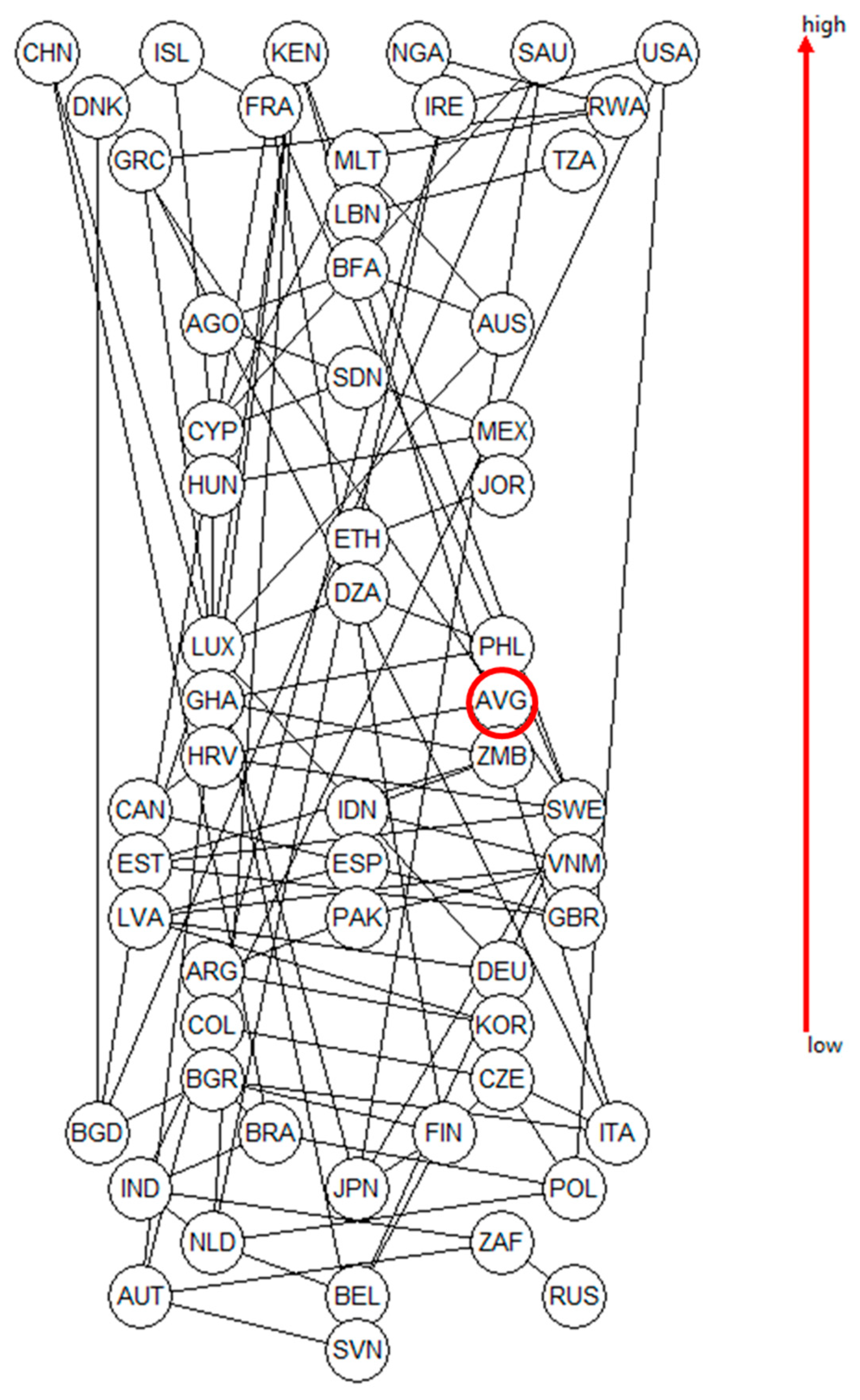
Turning to partial ordering, the MIS given in Table 1 (excluding the last column (the sum), as well as the grand total) leads to the Hasse diagram displayed in Figure 1. The level structure of the diagram gives a first indication of the mutual rankings of the 78 countries, plus the average, with the “good” countries being found at the bottom of the diagram and the “bad” countries being found at the top. Not surprisingly, the average of the 78 countries is found in the middle of the diagram. Apart from the overall ranking, the Hasse diagram is a visualization of which countries can be compared to each other (connected by lines) and which countries that, due to conflicting indicator values (cf. Equation (1)), are incomparable.

The diagram consists of 937 comparabilities and 716 incomparabilities due to the overall indicator pattern. It is worth noting here that the diagram is rather slim with 25 levels; this is a result of the high number of countries and only three indicators.

Looking at the figures in Table 1, it is not surprising that the HHW indicator plays a dominating role. This is substantiated by calculating the indicator’s importance. Hence, the relative importance of the three indicators [20] is found to be 0.723, 0.169, and 0.108, for HHW, FSW, and ReW, respectively.

3.1. Average Ranking

Due to the number of incomparabilities, as displayed in the Hasse diagram (Figure 1), it is not immediately possible to obtain a strict linear order unless a composite indicator is generated, e.g., through a simple arithmetic addition of each of the three indicators. This process is often applied, as such a linear order is typically desired. However, such an aggregation will mask the influence of each of the indicators and will, more seriously, result in compensation effects, where one high indicator value will be compensated by other low values [27]. Here, the average rankings [21,22] come into play. In

Table 3. Average ranks of the 78 countries plus the average based on equal weights for the three indicators (for country codes, cf. Table 1).

Country	LPOMext	Rank
NGA	57,791	58
RWA	56,582	57
TZA	55,275	56
LBN	53,991	55
ISL	53,635	54
BFA, COG, MDG, MWI, MLI, MOZ, NER, SLE, UGA	52,708	53
SAU	51,641	52
AGO, CMR, CIV, SEN, ZWE	51,364	51
SDN	50,048	50
MLT	49,255	49
MEX	48,647	48
USA	4752	47
JOR, TUR	47,182	46
KEN	46,086	45
ETH	45,757	44
CHN	44,625	43
DZA, EGY, MAR, TUN	44,332	42
PHL	42,832	41
GHA	41,145	40
GRC	39,749	39
ZMB	39,169	38
FRA	39,111	37
DNK	38,389	36
IDN	37,332	35
CYP, ARE	3715	34
AVG	35,716	33
VNM	35,223	32
HUN	33,696	31
PAK	32,904	30
ARG	30,798	29
AUS	30,426	28
IRE	30,102	27
COL	28,353	26
HRV, PRT	28,309	25
BGR	2572	24
CAN	25,511	23
ESP	22,189	22
BRA	2055	21
LVA, LTU	19,155	20
IND	16,397	19
SWE	16,187	18
KOR	15,767	17
LUX	15,676	16
CZE, ROU, SVK,	13,514	15
ZAF	12,036	14
FIN	8263	13
POL	7646	12
EST	7179	11
BGD	6304	10
AUT	5442	9
NLD	5073	8
RUS	4969	7
ITA	3994	6
DEU	3722	5
GBR	3465	4
BEL	3035	3
JPN	291	2
SVN	1349	1

, the average rankings of the 78 countries, plus the average, is shown, with the left column indicating equivalent countries.

In Table 3, it can be immediately seen that the three countries with the highest food waste per capita are Nigeria, Rwanda, and Tanzania. These are countries with a high degree of undernourishment, approx. 12% in Nigeria [28] and more than 35% in Rwanda [29]. However, at the same time, these figures appear to be closely connected to an extreme loss of food during production [28,29]. Thus, both Nigeria [28] and Rwanda [29] lose and waste around 40% of their total food production, corresponding to 31% [28] and 21% [29] of the total production areas, respectively. In Tanzania, about 25% is lost during production and a further 15% is lost during storage, typically due to insect damage [30].

On the other end of the scale, we find Belgium, Japan, and Slovenia with the lowest overall food waste per capita, i.e., 80, 88, and 61 kg of food waste per capita, respectively. Although still considerable amounts, these values are low. For all three countries, it can be noted that the ReW values in particular are very low, and for Slovenia and Belgium, the HHW values are extremely low, at only 34 and 50 kg per capita, respectively. For all three countries, the FSW is at the lower end of the scale, with 20, 15, and 20 kg per capita, respectively (Table 1).

As mentioned above, the data may be subject to uncertainty [1]. To elucidate the effect on the average ranking, a calculation was made, where an uncertainty (equal distribution) of 10% was included for the data [31]. Not surprisingly, this had some effect on the ranking. However, the overall picture did not change significantly. Hence, the top 10 countries with the highest food waste were, based on 10.000 Monte Carlo simulations, COG < MLI < UGA < BFA < LBN < SAU < TZA < RWA < ISL < NGA, and the bottom 10 of the list, i.e., the 10 countries with the lowest food waste, were SVN < JPN < GBR < BEL < EST < ITA < DEU< BGD < RUS < NLD.

3.2. Peculiar Countries

It can be immediately seen from the figures in Table 1 and the relative indicator importance that the food waste problem is mostly associated with HHW. However, a study on the possible so-called peculiar countries [23] may elucidate whether some countries fall outside of this general trend.

Based on the calculations, only two countries are classified as peculiar, i.e., the USA and Ireland, where, in both cases, the indicator profile appears to be (0,1,0). This can be interpreted as a peculiarity due to either high FSW values and/or low HHW and ReW values; which is nicely substantiated by the data in Table 1, displaying FSW values of 64 and 56 kg per capita, respectively, both significantly higher than the average FSW value of 27.06 kg per capita. At the same time, the HHW data at the lower end of the scale (Table 1) are in agreement with the fact that that a major proportion of food is not produced at home.

The explanation for this may be sought in the eating patterns of these countries. Pre-COVID, a report stated that Americans ate out at an average of 5.9 times per week [32]. A study from Ireland reported that more than 30% of the Irish population consumed takeaway food and ate at cafes at least once a week, in addition to eating at restaurants (21%) and pubs (15%) [33]. Hence, a major proportion of food originates from food services, and, thus, obviously, a major proportion of the food waste in these countries originates from FSW.

3.3. Influences of Different Weighting Schemes

In the recent report by The Economist [6], two different weighting schemes are mentioned. The weighting schemes attach specific weights to each of the indicators in order to reflect their importance. Thus, one scheme corresponds to the above analyses; i.e., all three indicators are assumed to have an equal weight of 0.33. The second scheme, as proposed by The Economist, favors HHW, with the weighting scheme being 0.5, 0.25, and 0.25 for MMW, FSW, and ReW, respectively.

Applying the 0.5, 0.25, and 0.25 weighting scheme changed the average rankings significantly. Thus, the top, ten countries with the highest food waste were found to be DZA > AGO > ARG > AUS > AUT > BGD > BEL > BRA > BGR> BFA, whereas the bottom ten with the lowest food waste were TZA > TUN > TUR > ARE > UGA > GBR > USA > VNM > ZMB > ZWE. Taking the USA as an illustrative case, if applying the ranking based on equal weighting, the USA ranks at place 47, whereas if applying the 0.5, 0.25, and 0.25 weighting scheme, the USA drops to rank 75; i.e., the USA becomes the country with the fourth lowest food waste. To explain this fact, the relative importance of the three indicators should be brought into play. For the USA, in the original scheme, i.e., the equal weighting scheme, the relative importance of the HHW, FSW, and ReW was 0.424, 0.460, and 0.115, respectively, whereas in the case of the 0.5, 0.25, and 0.25 weighting scheme, the relative importance was found to be 0.600, 0.323, and 0.081, respectively. Hence, the influence of the high FSW was reduced by assigning a lower weight to FSW.

The argument for the second weighting scheme may well be the dominance of HHW and that HHW in particular should be a subject for all households. However, there is no specific reason for choosing one scheme over the other. Thus, it appears appropriate to include both in an overall evaluation.

The GLA approach [18,19] is specifically designed to include several weighting schemes—for example, stakeholder opinions—without trying to force a joint agreement on one single weighting scheme. Thus, GLA includes all schemes simultaneously without any pretreatment or pooling, typically resulting in highly enriched Hasse diagrams that may facilitate possible decision processes. In the present case, the new Hasse diagram (not shown) has 1539 comparabilities and only 114 incomparabilities. In

Table 4. Average ranks of the top 10 and bottom 10 countries.

Country	Rank
TOP-10 (the “bad”):
NGA	58
ISL	57
RWA	56
TZA	55
MLT	54
USA	53
GRC	52
SAU	51
LBN	50
BFA, COG, MDG, MWI, MLI, MOZ, NER, SLE, UGA	49
BOTTOM-10 (the “good”):
ITA	10
NLD	9
EST	8
RUS	7
GBR	6
JPN	5
BEL	4
AUT	3
BGD	2
SVN	1

, the top 10 and the bottom 10 ranked countries are summarized.

Compared to Table 3, it can immediately be noted that, overall, there were only minor differences between the ranking based on weighting scheme 1 (equal weights) from the ranking following the GLA procedure, although the specific rankings were different. Thus, the USA found its place in the top 10 group, and Israel moved to the second position. Analogously, the individual rankings in the bottom 10 group changed, but, virtually, the group remained the same.

4. Conclusions and Outlook

At close to 1 billion tons worldwide, food waste is a serious global problem, as the figure suggests that 25–30% of all food produced is never eaten [34]. Further, this is associated with around 8–10% of annual global greenhouse gas emissions [34]. Rather ambitiously, Sustainable Development Goal 12.3 states that “by 2030, (to) halve per capita global food waste at the retail and consumer levels and reduce food losses along production and supply chains, including post-harvest losses.” [35]. To eventually comply with SDG 12.3, all countries need to focus on the reduction of food waste in all sectors.

The present study describes data analyses of 78 countries around the world based on the available data on food waste separated into three categories, i.e., household waste (HHW), food service waste (FSW), and retail waste (ReW).

On average, the 78 countries examined in the present paper waste 12,706 kg of food per capita according to the 2021 Food Sustainability Index [1,6]. The three food waste categories, namely, household waste (HHW), food service waste (FSW), and retail waste (ReW), are responsible for approx. 67%, 21%, and 12% of food waste, respectively. Based on these figures, it is not surprising that HHW appears to be the most important factor, as verified by a sensitivity analysis. It should be remembered that the figures include the amount of inedible parts [1], which may be significantly different among the countries due to differences in diet and the availability of food products. Thus, the figures for low-income countries may, to some extent, be misleading as a result of food with a higher amount of inedible parts.

The data analyses were performed by applying various methodologies of the partial order concept. Hence, an average ranking based on all three indicators (HHW, FSW, and ReW) of the 78 countries gave an insight into the “good” countries, such as Belgium, Japan, and Slovenia, and the “bad” countries, such as Nigeria, Rwanda, and Tanzania.

A special analysis found the USA and Ireland to be so-called peculiar countries, as these two countries were rationalized by very high FSW values. This is because a major proportion of the daily food of the average population of these countries is consumed outside the home or as a takeaway.

Considering that the world today produces enough food for everyone, while, at the same time, 829 million people worldwide go to bed hungry on a daily basis and around 14 million children under five suffer from severe stunting [35], it may seem too polite to distinguish between good and bad countries; maybe they all ask for the label “ugly”. The objective of SDG 12.3 to halve food loss by 2030 [35] seems to be rather difficult to achieve, as “Globally, food loss estimates have remained steady between 2016 and 2020, although with substantial variations across regions and subregions” [35], with both social and environmental challenges pending.

The application of a partial order methodology has been described in several papers, and it has shown its potential, e.g., as a decision support tool, in a wide variety of research fields; an extensive bibliography can be found in [25]. In the present paper, the retrieved rankings indicate that all countries are facing comprehensive tasks to reduce food waste and, thus, to combat social, health-related, and environment problems.

References

- United Nations Environment Programme. Food Waste Index Report 2021. Nairobi. 2021. Available online: https://www.unep.org/resources/report/unep-food-waste-index-report-2021 (accessed on 29 August 2022).
- McCarthy, N. The Enormous Scale of Food Waste, Forbes. 2021. Available online: https://www.forbes.com/sites/niallmccarthy/2021/03/05/the-enormous-scale-of-global-food-waste-infographic/ (accessed on 29 August 2022).
- Tomaszewska, M.; Bilska, B.; Kołożyn-Krajewska, D. Food Waste in Catering Establishments—An Analysis of Causes and Consequences. Eur. J. Sustain. Dev. 2021, 10, 365–375. [Google Scholar] [CrossRef]
- Bilska, B.; Tomaszewska, M.; Kołożyn-Krajewska, D. The Management of Meals in Food. Service Establishments in the Context of FoodWaste—Results of Focus Group Interviews with Employees and Owners. Sustainability 2022, 14, 9258. [Google Scholar] [CrossRef]
- Baig, M.B.; Alotaibi, B.A.; Alzahrani, K.; Pearson, D.; Alshammari, G.M.; Shah, A.A. Food Waste in Saudi Arabia: Causes, Consequences, and Combating Measures. Sustainability 2022, 14, 10362. [Google Scholar] [CrossRef]
- The Economist, The Food Sustainability Index 2021. Available online: https://impact.economist.com/projects/foodsustainability (accessed on 29 August 2022).
- Annoni, P.; Bruggemann, R.; Carlsen, L. A multidimensional view on poverty in the European Union by partial order theory. J. Appl. Stat. 2015, 42, 535–554. [Google Scholar] [CrossRef]
- Bruggemann, R.; Patil, G.P. Ranking and Prioritization for Multi-indicator Systems—Introduction to Partial Order Applications; Springer: New York, NY, USA, 2011. [Google Scholar]
- Bruggemann, R.; Voigt, K. Basic Principles of Hasse Diagram Technique in Chemistry. Comb. Chem. High Throughput Screen. 2008, 11, 756–769. [Google Scholar] [CrossRef] [PubMed]
- Carlsen, L. Happiness as a sustainability factor. The World Happiness Index. A Posetic Based Data Analysis. Sustain. Sci. 2018, 13, 549–571. [Google Scholar] [CrossRef]
- Carlsen, L.; Bruggemann, R. Partial order methodology a valuable tool in chemometrics. J. Chemom. 2013, 28, 226–234. [Google Scholar] [CrossRef]
- Carlsen, L. Bruggemann, R. The “Failed State Index” Offers More than Just a Simple Ranking. Soc. Indic. Res. 2014, 115, 525–530. [Google Scholar] [CrossRef]
- Carlsen, L.; Bruggemann, R. Environmental perception in 33 European countries an analysis based on partial order. Environ. Dev. Sustain. 2018, 22, 1873–1896. [Google Scholar] [CrossRef]
- Newlin, J.; Patil, G.P. Application of partial order to stream channel assessment at bridge infrastructure for mitigation management. Environ. Ecol. Stat. 2010, 17, 437–454. [Google Scholar] [CrossRef]
- Voigt, K.; Bruggemann, R.; Scherb, H.; Cok, I.; Mazmanci, I.; Mazmanci, A.; Turgut, C.; Schramm, K.-W. Organochlorine Pesticides in the Environment and Humans Necessity for Comparative Data Evaluation. In Simulation in Umwelt- und Geowissenschaften; Workshop Leipzig, Wittmann, J., Müller, M., Eds.; Shaker-Verlag: Aachen, Germany, 2013; Available online: https://www.amazon.co.uk/Simulation-Umwelt-Geowissenschaften-Workshop-Leipzig/dp/3844020098 (accessed on 29 August 2022).
- Bruggemann, R.; Carlsen, L. (Eds.) Partial Order in Environmental Sciences and Chemistry; Springer: Berlin, Germany, 2006; Available online: https://www.springer.com/gp/book/9783540339687 (accessed on 29 August 2022).
- Bruggemann, R.; Carlsen, L. Introduction to Partial Order Theory Exemplified by the Evaluation of Sampling Sites. In Partial Order in Environmental Sciences and Chemistry; Bruggemann, R., Carlsen, L., Eds.; Springer: Berlin, Germany, 2006; pp. 61–110. [Google Scholar]
- Carlsen, L.; Bruggemann, R. Partial Order as Decision Support Between Statistics and Multi-criteria Decision Analyses. Standards 2022, 2, 22. [Google Scholar] [CrossRef]
- Carlsen, L.; Bruggemann, R. Combining different stakeholders’ opinions in multi-criteria decision analyses applying partial order methodology. Standards 2022, 2, 35. [Google Scholar] [CrossRef]
- Bruggemann, R.; Münzer, B. A Graph-Theoretical Tool for Priority Setting of Chemicals. Chemosphere 1993, 27, 1729–1736. [Google Scholar] [CrossRef]
- Bruggemann, R.; Voigt, K. An Evaluation of Online Databases by Methods of Lattice Theory. Chemosphere 1995, 31, 3585–3594. [Google Scholar] [CrossRef]
- Bruggemann, R.; Halfon, E.; Welzl, G.; Voigt, K.; Steinberg, C.E.W. Applying the Concept of Partially Ordered Sets on the Ranking of Near-Shore Sediments by a Battery of Tests. J. Chem. Inf. Comput. Sci. 2001, 41, 918–925. [Google Scholar] [CrossRef] [PubMed]
- Bruggemann, R.; Carlsen, L. An Improved Estimation of Averaged Ranks of Partial Orders. MATCH Commun. Math. Comput. Chem. 2011, 65, 383–414. Available online: https://match.pmf.kg.ac.rs/electronic_versions/Match65/n2/match65n2_383-414.pdf (accessed on 29 August 2022).
- Bruggemann, R.; Annoni, P. Average Heights in Partially Ordered Sets. MATCH Commun. Math. Comput. Chem. 2014, 71, 117–142. Available online: http://match.pmf.kg.ac.rs/electronic_versions/Match71/n1/match71n1_117-142.pdf (accessed on 29 August 2022).
- Bruggemann, R.; Carlsen, L. Incomparable—What now? MATCH Commun. Math. Comput. Chem. 2014, 71, 694–716. [Google Scholar]
- Bruggemann, R.; Carlsen, L.; Voigt, K.; Wieland, R. PyHasse Software for Partial Order Analysis. In Multi-Indicator Systems and Modelling in Partial Order; Bruggemann, R., Carlsen, L., Wittmann, J., Eds.; Springer: New York, NY, USA, 2014; pp. 389–423. [Google Scholar] [CrossRef]
- Munda, G. Social Multi-Criteria Evaluation for a Sustainable Economy; Springer: Berlin/Heidelberg, Germany, 2008; Available online: https://www.springer.com/la/book/9783540737025 (accessed on 29 August 2022).
- Nigeria Food Smart Country Diagnostic. Available online: https://openknowledge.worldbank.org/bitstream/handle/10986/34522/Nigeria-Food-Smart-Country-Diagnostic.pdf?sequence=1&isAllowed=y (accessed on 19 August 2022).
- Rwanda Food Smart Country Diagnostic. Available online: https://openknowledge.worldbank.org/bitstream/handle/10986/34523/Rwanda-Food-Smart-Country-Diagnostic.pdf?sequence=1&isAllowed=y (accessed on 29 August 2022).
- Talking about Food Loss and Food Waste with Dr Christopher Mutungi, IITA Food Technology Specialist. Available online: https://www.iita.org/news-item/talking-about-food-loss-and-food-waste-with-dr-christopher-mutungi-iita-food-technology-specialist/ (accessed on 29 August 2022).
- Available online: https://www.businessinsider.com/what-people-spend-on-dining-out-2019-8?r=US&IR=T (accessed on 19 August 2022).
- Out of Home Eating National Survey 2020. Available online: https://www.failteireland.ie/FailteIreland/media/WebsiteStructure/Documents/2_Develop_Your_Business/Failte-Ireland-Out-of-Home-Eating-Research-FINAL-VERSION.pdf (accessed on 29 August 2022).
- United Nations Intergovernmental Panel on Climate Change. Special Report on Climate Change and Land. Chapter 5: Food Security. 2019. Available online: https://www.ipcc.ch/site/assets/uploads/2019/08/2f.-Chapter-5_FINAL.pdf (accessed on 29 August 2022).
- Indicator 12.3.1 Global Food Loss and Waste. Available online: https://www.fao.org/sustainable-development-goals/indicators/1231/en/ (accessed on 29 August 2022).
- Action Against Hunger. Available online: https://www.actionagainsthunger.org/world-hunger-facts-statistics (accessed on 29 August 2022).
Figure 1.
Hasse diagram showing the partial ordering of the 78 countries, plus the average, based on the three indicators HHW, FSW, and ReW (cf. Table 1). For “identical” countries, only one representative is shown.