Article

Location Allocation of Biorefineries for a Switchgrass-Based Bioethanol Supply Chain Using Energy Consumption and Emissions

1
Department of Management, Marketing and Operations, College of Business, Embry-Riddle Aeronautical University, Daytona Beach, FL 32114, USA
2
Department of Decision and Information Sciences, School of Business Administration, Oakland University, Rochester, MI 48309, USA
3
Nicolais School Business, Wagner College, Staten Island, NY 10301, USA
4
Transportation, Logistics, and Finance Department, College of Business, North Dakota State University, Fargo, ND 58108, USA
5
Upper Great Plains Transportation Institute, North Dakota State University, Fargo, ND 58108, USA
6
School of Business, Widener University, Chester, PA 19013, USA
*
Author to whom correspondence should be addressed.
Logistics 2023, 7(1), 5; https://doi.org/10.3390/logistics7010005
Submission received: 1 July 2022 / Revised: 30 December 2022 / Accepted: 5 January 2023 / Published: 17 January 2023

Abstract

:
Background: Due to the growing demand for energy and environmental issues related to using fossil fuels, it is becoming tremendously important to find alternative energy sources. Bioethanol produced from switchgrass is considered as one of the best alternatives to fossil fuels. Methods: This study develops a two-stage supply chain modeling approach that first determines feasible locations for constructing switchgrass-based biorefineries in the state of North Dakota by using Geographic Information Systems (GIS) analysis. In the second stage, the profit of the corresponding switchgrass-based bioethanol supply chain is maximized by developing a mixed-integer linear program that aims to commercialize the bioethanol production while impacts of energy use and carbon emission costs on the supply chain decisions and siting of biorefineries are included. Results: The numerical results show that carbon emissions and energy consumption penalties affect optimal biorefinery selections and supply chain decisions. Conclusions: We conclude that there is no need to penalize both emissions and energy use simultaneously to achieve desirable environmental benefits, otherwise, the supply chain becomes non-profitable. Moreover, imposing emissions or energy consumption penalties makes the optimization model closer to supply sources while having higher land rental costs. Such policies would promote sustainable second-generation biomass production, thus decreasing reliance on fossil fuels.

1. Introduction

The transportation sector’s reliance on nonrenewable fuel sources, as well as the severe social and environmental implications, raised research motives in the field of biofuel production [1,2,3]. Biofuels, such as bioethanol, are made from renewable biomass feedstocks, such as energy crops, forest wastes, and agricultural residues. Because of their tremendous potential to reduce environmental pollution, biofuels were regarded as promising alternatives to fossil-based fuels for the sustainable development of the global economy [4]. Biofuels rely heavily on biomass feedstock, a dispersed resource whose availability depends on geographical location. However, due to their lower carbon emission generation compared to fossil-based fuels, they are considered important sources of renewable energy [5].
As a type of biofuel, bioethanol can be used as a fuel in various percentages when blended with gasoline [6]. Over the past decade, there was a significant increase in the production of first-generation bioethanol from food crops such as corn. However, the growing production raised serious concerns regarding the shortage of corn-based foods [7]. Thus, researchers and practitioners recently considered producing bioethanol from second-generation biomass (especially lignocellulosic biomass), such as switchgrass. Switchgrass is known as one of the most promising resources to produce second-generation bioethanol [8,9]. With its high yields, low soil erosion, low incidence of pests and diseases, and low water and nutrient requirements, switchgrass has great potential for bioethanol production in different geographical regions (marginal lands) [2]; hence, its cultivation creates new jobs in locations where there is insufficient fertile soil for agricultural production [9,10].
The United States enacted several legislations to encourage the production of second-generation bioethanol and to cap production of first-generation bioethanol from corn starch [11]. According to the Renewable Fuel Standard (RFS), 36 billion gallons of biofuels must be produced annually, while only 15 billion gallons can be produced from corn starch. Of the remaining 21 billion gallons per year (BGPY), cellulosic bioethanol should account for at least 16 BGPY [7]. With the second-generation bioethanol being essential, it is crucial to make its production profitable. In addition to economic benefits, maximizing environmental performance, such as reducing energy consumption and emission levels, is becoming increasingly important [12,13]. Therefore, it is necessary to balance activities across a bioethanol supply chain to maximize its profit while minimizing environmental and energy costs. The biofuel supply chain network design approach provided solutions to the analytical needs mentioned above.
In a comprehensive review, Ghaderi et al. [14] concludes that the literature focuses primarily on processing and manufacturing sites, whereas new research is needed to consider all the echelons of the supply chain, as well as the interactions between them. As biomass feedstocks are widely dispersed and low density, transporting them will be costly, which will complicate the design of biofuel supply chains. To ensure the sustainability of a biofuel supply chain, it is imperative that biorefineries are located within a reasonable distance of both their supply and demand nodes. There were several studies conducted to determine optimal designs of the biofuel supply chain networks. Babazadeh et al. [15] developed a model for designing a biodiesel supply chain, which determined the optimal numbers, locations, and capacities of production facilities, as well as transportation modes, technologies, and production plans. Ebrahimi et al. [16] developed a supply chain network to produce renewable jet fuel in Alabama, Florida, and Georgia. The optimal locations for setting up biorefineries were found while maximizing supply chain profits. The optimization of biofuel supply chains with consideration of economic, energy, and environmental aspects, emerged as a more holistic approach to designing biofuel supply chain networks, as it can assist decision makers in developing sustainable biofuel supply chains that meet multiple objectives [4]. By including emissions costs in their model, Haji Esmaeili et al. [17] designed a supply chain network to find optimal locations for biorefineries in North Dakota. Their results indicate that switchgrass is an economically and environmentally better alternative to corn stover for the production of bioethanol. Ghaderi et al. [6] proposed a multi-objective robust possibilistic programming model for designing a sustainable switchgrass-based bioethanol supply chain (SBSC) network under epistemic uncertainties, while considering environmental and social life cycle analyses. However, only a few studies examined energy consumption and CO2e emissions simultaneously in designing a biofuel supply chain. Gonela et al. [18] proposed stochastic mixed-integer linear programing (MILP) to design a hybrid generation bioethanol supply chain that maximized supply chain profit while considering greenhouse gas (GHG) emissions, irrigation, land-use restrictions, and energy efficiency in their model. Additionally, Ren et al. [4] developed a life cycle energy and emissions optimization model for designing a biofuel supply chain without considering logistics expenses. Using multiple feedstock models, they examined the optimal amount of energy and carbon emissions from a first-generation biomass feedstock. However, these studies did not conduct sensitivity analysis for energy use and emission penalties to investigate how these two environmental factors could affect the location of biorefineries. The economic and environmental aspects of biofuel supply chain networks were only superficially explored in many regional and local studies. However, policy makers and planners need site-specific studies to assist with local and regional planning [19].
To facilitate access to farmers, work force, and biomass feedstocks, biofuel producers often build biorefineries near supply zones, highways, railroads, and large cities, maximizing environmental and social advantages [1,20]. As a result, locating biorefineries based only on economic criteria, such as minimizing transportation costs, would fail to meet the environmental and social advantages of biofuel production [20,21]. There are few studies on the biofuel supply chain network design that determined the suitability of the potential locations to establish biorefineries using GIS analysis [19]. In an analysis of the biofuel supply chain network design, Zhang et al. [1] utilized GIS in conjunction with optimization models to design a biofuel supply chain network and minimize the total system costs. Similarly, Sanchez-Garca et al. [22] used a GIS optimization model to identify the optimal site for a wood-fired power plant, which minimized supply chain costs and greenhouse gas emissions.
To overcome the aforementioned research gaps, this study employs a two-stage decision-making approach to design a SBSC network in the state of North Dakota. The following are the contributions of this research to the literature:
  • Locating potential biorefineries using GIS.
    -
    Several studies simplified the identification of potential biorefineries by selecting only centroids, city gates, etc., whereas very few studies used Geographic Information Systems to specify potential locations more realistically. Employing GIS analysis, we considered geographical factors, such as distances from major cities, biomass feedstock suppliers, water sources, highways, and railroads, to locate potential biorefineries.
  • Developing a MILP model to maximize the profit while considering the impacts of energy use and carbon emissions throughout the supply chain.
    -
    Our model is significant in considering the joint impacts of carbon emissions and energy consumption on the design of a biofuel supply chain.
  • Providing a detailed analysis of how penalties associated with carbon emissions and energy consumption in the supply chain could impact its design and profitability.
    -
    Few studies were conducted that provide detailed supply chain planning and design scenarios based on the penalties set for carbon emissions and energy consumption within biofuel supply chains. In this study, we show how different penalties for energy consumption and carbon emissions can affect location allocation of biorefineries and supply chain planning.

2. Materials and Methods

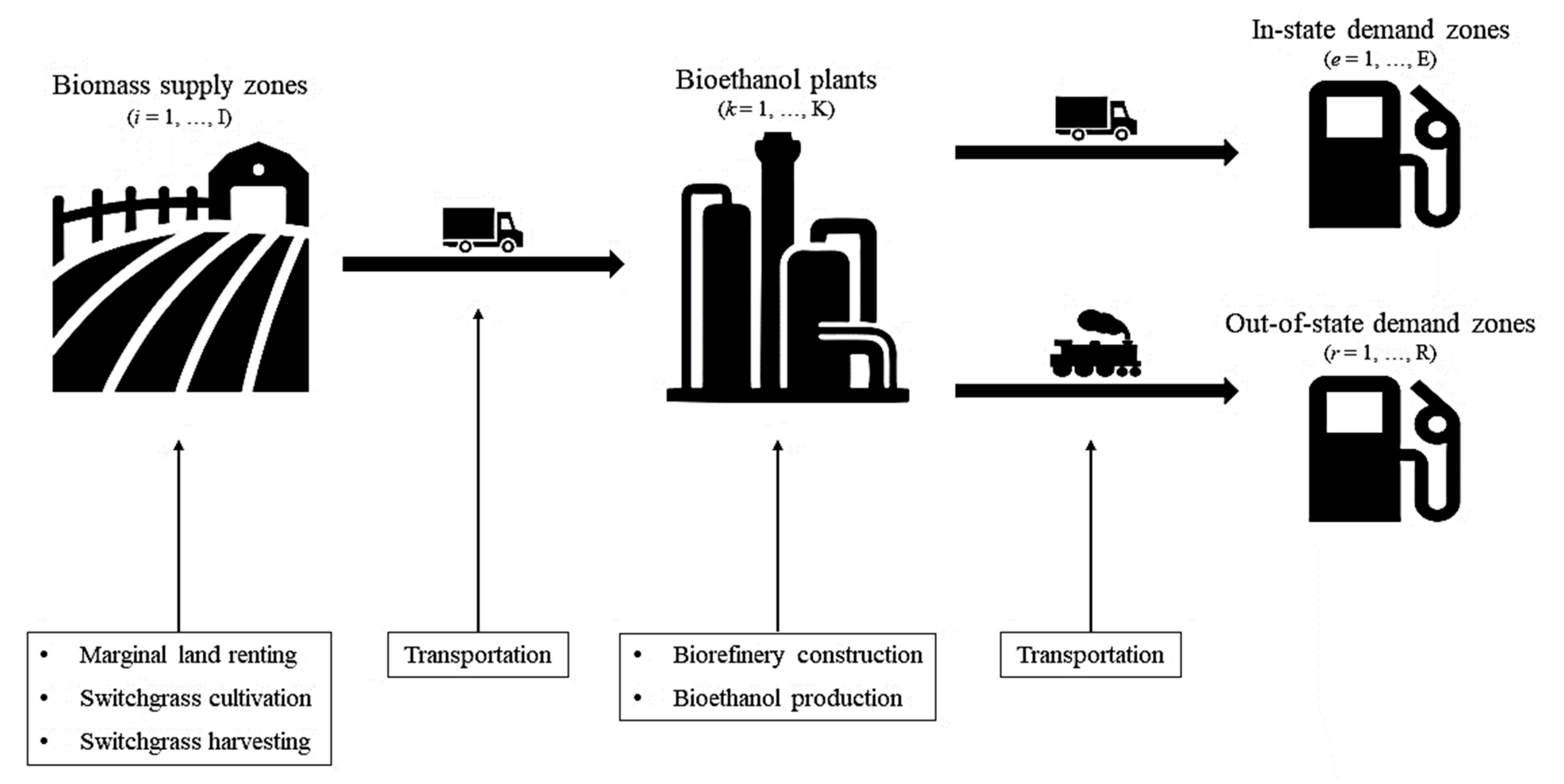
2.1. Problem Statement

This study aims to design a sustainable SBSC network by developing a two-stage modeling approach. In the first stage, we determine a group of feasible (suitable) locations for biorefineries, and in the second stage, we design a supply chain that can maximize profits and determine optimal biorefinery locations. The SBSC network includes three major parts: biomass supply zones (suppliers), bioethanol plants (biorefineries), and in-state and out-of-state demand zones. The SBSC network and its associated activities within each part are shown in Figure 1. The biomass feedstock (switchgrass) flows from the suppliers to the bioethanol plants (biorefineries) by truck. Then the bioethanol produced in plants either goes to in-state demand zones by truck or to out-of-state demand zones by rail.
This study examines the SBSC in the state of North Dakota as a case study. The environmental, temperature, and soil conditions in the Northern Great Plains of the United States, where North Dakota is located, are suitable for growing commercial switchgrass [2]. Biomass supply zones comprise the first echelon of the SBSC network flow where marginal lands are located. Marginal lands almost exist in all 53 counties of North Dakota; thus, switchgrass can be cultivated all over the state. These counties were divided into nine agricultural statistical districts (ASDs), including NW, NC, NE, WC, Central, EC, SW, SC, and SE serving as switchgrass suppliers in the design of the SBSC network [16,17]. Figure 2 shows the switchgrass supply zones and North Dakota infrastructure considered for designating possible bioethanol plants. This figure shows highly populated cities, lakes, rivers, roads, railroads, and ASDs colored according to their potential for switchgrass cultivation. The shapefiles used to create the GIS map was extracted from the United States Census Bureau [23].
The capacity of switchgrass-based biorefineries was set at 150 million gallons per year (MGPY), which is the maximum capacity for commercialized cellulosic biorefineries [24]. Moreover, Table 1 shows the total marginal lands available for switchgrass cultivation in the ASDs along with their rental costs. According to the United States Department of Agriculture (USDA), cropland, pastureland, and marginal land accounted for 69.1%, 26.1%, and 4.8% of the 15.89 million hectares of total farmland under cultivation in North Dakota [25]. This study focuses only on the marginal land for switchgrass cultivation which totals around 0.76 million hectares. Considering marginal lands for switchgrass cultivation avoids competition for lands used for food and feed crops. Since marginal lands were not used previously, there is no documented marginal land rental cost; therefore, we used the pastureland rental cost for each supply zone as the cost for renting marginal land.
The bioethanol produced in North Dakota is sold to fulfill both in-state and out-of-state demands in the United States. According to our conversations with bioethanol experts in ND, there are six in-state demand zones, including Fargo, Grand Forks, Jamestown, Bismarck, Dickinson, and Minot, which have fuel racks where bioethanol is blended with gasoline. Additionally, there are four out-of-state demand zones, including Houston (TX), Los Angeles (CA), Portland (OR), and Seattle (WA), for the bioethanol produced by biorefineries located in North Dakota. Our case study becomes more realistic by considering out-of-state demand zones, allowing policymakers to depend on the corresponding conclusions. The majority (90%) of North Dakota’s bioethanol production is transported by rail to other states, with only 10% of it being sold locally (transported by truck) [26]. Accordingly, the demand associated with each demand zone is assigned in proportion to its population. The in-state and out-of-state demand zones are shown in Figure 3.

2.2. Methodology

This section explains the two-stage modeling approach developed to design an SBSC network. In the first stage, GIS analytics uses the topography and geographical factors in North Dakota to determine the feasible locations for building biorefineries. These factors were highlighted in earlier literature on the selection of appropriate sites for establishing biorefineries [1,27]. The factors are presented in the following:
  • Locations within one mile of a state or federal road transport infrastructure;
  • Locations within one mile of a rail transportation network;
  • Areas near towns or cities having a population of at least 2000;
  • Areas within a quarter-mile and one mile of a waterbody (rivers, lakes, etc.);
  • Locations with rich supplies of switchgrass biomass.
These geographical factors are the main drivers in finding potential locations for building biorefineries as they enhance long term social, environmental, and human resource benefits for the stakeholders [1,27]. For instance, it is essential to locate biorefineries at locations where both rail and road are available for facilitating the transportation of switchgrass and the distribution of bioethanol. A large population is also crucial to assure the labor availability for facilities. Locations close to a waterbody are also preferable for biorefineries to minimize variable operating costs [27]. Furthermore, locations adjacent to supply zones with abundant supplies of switchgrass are preferred to reduce transportation costs, emissions, and energy consumption [28].
The results from the GIS analysis are used in the second stage of the decision-making approach in which we use a MILP model that maximizes the profit of the SBSC network. In the model, the number of biorefineries is considered a binary variable, while other variables are considered continuous. The objective function of the optimization model includes revenues from bioethanol and switchgrass-based bioethanol co-product (which is called lignin pallet) sales; cultivation and harvesting costs of switchgrass, transportation expenses due to shipping switchgrass to biorefineries and shipping bioethanol to demand zones, production and construction costs of bioethanol plants, and finally, penalties associated with energy consumption and carbon emissions of the supply chain activities. The optimization model determines the optimal biorefinery locations from the potential locations provided by the GIS analysis, while minimizing transportation costs, energy consumption, and carbon emissions. Accordingly, the model assigns the optimal supplier(s) and demand zone(s) to each biorefinery. It should be noted that the effects of both economic and environmental factors on supply chain decisions will be considered simultaneously.
For the proposed model, we make the following assumptions: (1) the bioethanol producers are responsible for switchgrass procurement (acquisition) including renting marginal lands, the cultivation and harvesting process, and shipment of switchgrass [17]; (2) the bioethanol producers are also responsible for bioethanol transport but not for switchgrass-based bioethanol co-product [17]; and (3) all the bioethanol produced to meet a specific demand level are sold to the demand nodes [16,17,28].
The notations, parameters, and decision variables of the optimization model are presented in Table 2 and the input parameters are shown in Table A1 in Appendix A.
The objective function used in this study to address decisions is as follows:
M a x   Z = π ( k K e E X k e + k K r R Z k r ) + φ . C P 1 λ i I k K r i . Q i k v . i I k K Q i k h . i I k K Q i k i I k K γ g + η g . d i k Q i k f b . k K Y k ρ k K e E X k e + k K r R Z k r e E k K γ t + η t . d k e X k e k K r R γ r + η r . d k r Z k r ξ ( A C E . i I k K Q i k + S T E . i I k K d i k . Q i k + P R E k K e E X k e + k K r R Z k r + B T E . k K e E d k e . X k e + B R E . k K r R d k r . Z k r ) ψ ( A C G . i I k K Q i k + S T G . i I k K d i k . Q i k + P R G k K e E X k e + k K r R Z k r + B T G . k K e E d k e . X k e + B R E . k K r R d k r . Z k r )
The objective function in Equation (1) maximizes profit (revenue–cost) for the SBSC. The first two elements in the objective function are supply chain revenues coming from two final products: bioethanol and switchgrass-based bioethanol co-product. Other elements in the objective function present the cost components of the model, including marginal land rental cost for switchgrass cultivation, switchgrass cultivation cost, switchgrass harvesting cost, transportation cost of switchgrass, biorefinery capital cost, biorefinery production cost, transportation cost of bioethanol via truck to in-state demand zones, transportation cost of bioethanol via rail to out-of-state demand zones, emissions cost, and energy cost. Supply chain emissions are penalized with a cost of ξ (carbon tax). The amount of CO2e emitted due to supply chain activities, such as switchgrass acquisition, bioethanol production, and switchgrass and bioethanol transportation, are considered as emission sources in the SBSC. The energy cost factor (ECF) ψ is set as a penalty for the total amount of energy consumed in the SBSC to reduce energy consumption. Switchgrass acquisition, bioethanol production, and switchgrass and bioethanol transportation are considered as sources of energy consumption in the supply chain.
The constraints of the model are shown in Equations (2)–(12):
k K Q i k λ · a i               i I
θ i I Q i k = e E X k e + r R Z k r           k K
6 k K e E X k e + k K r R Z k r = C P
e E X k e + r R Z k r C A P · Y k           k K
k K X k e = D E M e             e E
k K Z k r = D E M r             r R
Y k = 0 , 1             k K
C P 0
Q i k 0             i I ,   k K
X k e 0           k K ,   e E
Z k r 0             k K ,   r R
Constraint (2) forces the amount of switchgrass harvested at area i to be less than or equal to the maximum switchgrass available to be harvested on marginal lands for each zone. The material flow constraints for biomass-to-bioethanol are given in Equation (3), and biomass to bioethanol co-product is specified by Equation (4). Constraint (5) represents the capacity constraints of bioethanol plants (if activated). Constraint (6) assures that the volume of bioethanol produced in biorefineries fulfills the demand of in-state demand zones. Likewise, constraint (7) declares that the volume of bioethanol produced in biorefineries satisfies the demand from out-of-state demand zones. Finally, constraints (8)–(12) confirm the nature and non-negativity of variables used in the model. The MILP is solved via OpenSolver 2.9.0 using the COIN-OR Branch-and-Cut (CBC) optimization engine [29].

3. Results and Discussion

3.1. Location Allocation of Potential Biorefineries with GIS Analysis

The ideal locations to build new bioethanol plants in North Dakota were determined based on GIS analysis and served as input for the MILP model, which specifies which facilities should be opened to satisfy the demand. According to GIS analysis, there were four possible cellulosic biorefinery locations in North Dakota for switchgrass-based bioethanol production that meet the required criteria for building a new bioethanol plant. According to Figure 4, these locations are in Ward, Grand Forks, Richland, and Stutsman counties, which were chosen as biorefinery names accordingly. It was observed that the proposed biorefineries were distributed among different ASDs.

3.2. Maximizing Profit without Emissions and Energy Consumption Penalties

As discussed previously, we use 150 MGPY as the maximum capacity for a biorefinery. Therefore, the maximum amount of bioethanol that can be produced across the four possible sites in North Dakota is 600 MGPY. To examine the effects of demand variation, we consider four different demand levels (150, 300, 450, and 600 MGPY). This enables us to analyze how demand levels can affect bioethanol facility selection decisions. As shown in Figure 5, the contribution of different cost components is almost the same through four different demand levels. Considering different demand levels while setting the penalties for emissions and energy use to zero, the biorefinery construction cost has the highest percentage of cost, followed closely by bioethanol production cost. Two cost elements contributed 67.2% to the total supply chain cost, suggesting that finding cost-effective production facilities and technologies for biorefineries has a significant role in reducing the supply chain costs. Transportation and cultivation costs are also significant, while land rental and harvesting costs are the smallest. Overall, the costs increased in an almost linear fashion as the available capacity increased in the various capacity scenarios.
The supply chain could attain profits of USD 70.74 million, USD 141.87 million, USD 209.76 million, and USD 273.26 million at 150, 300, 450, and 600 MGPY demand fulfillment rates. Accordingly, the supply chain could profit USD 0.472, USD 0.473, USD 0.466, and USD 0.455 per gallon of bioethanol produced at fulfillment rates of 150, 300, 450, and 600 MGPY, respectively. Based on the results, supply chain profit was not significantly impacted by higher production capacity.
Table 3 shows the optimal assignment of supply and demand zones to bioethanol plants. When the annual demand is 150 MGPY, Ward is the first bioethanol plant chosen by the MILP. The Ward biorefinery is the first location where policymakers and investors can build a new cellulosic bioethanol plant, which has the lowest logistical costs compared to other locations identified by GIS analysis. The Ward biorefinery is in the NW district where it can supply all its required biomass feedstock from switchgrass cultivation lands in the NW and NC districts. When the demand level increases to 300 MGPY, the Stutsman biorefinery located in the Central district is selected as the second bioethanol plant to open. In this scenario, the EC district lands along with Central district lands are rented to fulfill the required biomass feedstock for the Stutsman biorefinery. In this situation, the Ward biorefinery tries to meet most of the demand of out-of-state demand zones, including Los Angeles, Portland, and Seattle, as well as Minot in North Dakota, and the Stutsman biorefinery seeks to mostly fulfill the in-state demand (all in-state demand zones except Minot) along with Houston and the remaining bioethanol needed for Los Angeles. When the demand level is increased to 450 MGPY, the Grand Forks biorefinery is opened in the NE district by the MILP as the third biorefinery. When the demand level is set to its maximum (600 MGPY), Richland biorefinery is opened in the SE district as the fourth biorefinery plant to produce biofuel from switchgrass cultivated in the SE and EC districts. In this scenario, all four potential biorefineries are opened and assigned their closest supplier and demand zones. There are three supplier districts, WC, SW, and SC, which are not used in the optimal solution, as the other six supplier districts can supply enough switchgrass to produce 600 MGPY bioethanol. This also means the marginal lands in North Dakota have the potential to produce more switchgrass than biorefineries in North Dakota can process. Overall, considering different demand levels indicates that the order priority for opening cellulosic biorefineries in North Dakota is Ward, Stutsman, Grand Forks, and Richland.

3.3. The Impact of a Carbon Tax on the Supply Chain

In this section, the emissions penalty is not set to zero in the objective function, however, the energy use penalty is set to zero. In our model, an emissions cost is incurred based on carbon emissions from biomass acquisition (such as cultivating, harvesting, and collecting), transportation from supplier districts to biorefineries, bioethanol production, and transportation between biorefineries and demand zones. By considering these four emission sources, our model assesses the effects of carbon emissions generated in the switchgrass-to-bioethanol process. The environmental cost per unit of CO2e (kg of CO2e) is imposed as a carbon tax.
To consider the effects of a carbon tax, five different scenarios are considered for the carbon tax rate in the presence of the four demand level scenarios to better analyze the impact of emissions on the supply chain and bioethanol plant siting decisions. In our study, biorefineries are responsible for paying the penalties to the government for emissions coming from all activities through the supply chain. The different carbon tax values are “No Penalty” with a USD 0 carbon tax, “Regular” with a USD 0.1231 carbon tax, which is based on an estimation of the environmental costs of CO2 emissions [30], “Reaction Point” with varied carbon tax according to the demand level, which is the minimum carbon tax for which the supply chain starts to react to the carbon tax and reduce its emissions, “Profit = $0” with varied carbon tax according to the demand level, which is the minimum carbon tax for which the total supply chain profit is USD 0, “Another Biorefinery Needed” with varied carbon tax according to the demand level, which is the minimum carbon tax for which the supply chain adds another biorefinery.
Table 4 demonstrates the effects of the different carbon tax rates on the total profit and total carbon emissions of the supply chain. When demand is 150 MGPY, the minimum carbon tax, which makes the supply chain reduce its emissions, is USD 1.06 per kg CO2e. In this case, emissions decreased by 2.9% and profit reduced by 6.8%. This means that reducing emissions through a carbon tax requires a 6.8% economic compensation. Furthermore, the maximum profit of the supply chain remains positive until a carbon tax of more than USD 1.82 is imposed. In this case, increasing the carbon tax does not reduce the emissions unless a very high carbon tax (at least USD 70/kg CO2e) is applied for which the model opens another biorefinery to reduce emissions. In this situation, there will be a reduction in emissions, but the supply chain is no longer profitable. When demand is 300 or 450 MGPY, the same trends are seen. The minimum carbon taxes, which result in the supply chain reducing emissions (“Reaction Point” scenario), are USD 0.22 and USD 0.21 per kg CO2e, respectively, for 300 and 450 MGPY. In these cases, emission reductions are 0.7% and 0.4%, while reductions in profit are 11.7% and 11.8%, respectively. This indicates that as demand increases, a greater loss in profit is necessary to reduce emissions. Similarly, the supply chain stops making a profit if the carbon tax is higher than USD 1.89 and USD 1.79, respectively, when demand is 300 and 450 MGPY without a decrease in emissions. Clearly, emissions are lower when a very high carbon tax is imposed, however, with such high carbon taxes, the supply chain does not make any profit. The carbon taxes that affect the selection of bioethanol plants under the “Another Biorefinery Needed” scenario are USD 280 and USD 445 for the demand of 300 and 450 MGPY, respectively. When demand is 600 MGPY, there is no decrease in emissions, since the supply chain is at its maximum capacity and there are no options to reduce emissions. All in all, the carbon taxes from “Reaction Point” scenarios show the most promise as the supply chain makes a profit while emissions decrease.
As shown in Table 5, the number of bioethanol plants under different demand scenarios is constant until a very high carbon tax (“Another Biorefinery Needed” scenario) is applied. Even when the supply chain stops making a profit, the emission cost is not high enough to beat the construction cost of another biorefinery. Under different demand scenarios, when the carbon tax reaches a very high level (“Another Biorefinery Needed” scenario), one more biorefinery will be opened. A thought-provoking point of Table 5 is that with the demand of 150 MGPY, when the carbon tax reaches the “Reaction Point” (USD 1.09/kg CO2e here), the model chooses the Stutsman biorefinery instead of Ward, which indicates the importance of demand level, besides carbon tax rate, for selecting bioethanol plants. On the other hand, from the results of Table 4, we concluded that the supply chain starts to reduce its emissions when the “Reaction Point” carbon tax scenario is implemented. The reason for this drop can be found in Table 6. Table 6 shows how emissions from different sources in the supply chain change for different carbon tax values with a demand under 300 MGPY. According to Table 6, emissions coming from the biomass acquisition process and bioethanol production are constant regardless of the carbon tax. However, emissions coming from the transportation of biomass from suppliers to biorefineries and the transportation of bioethanol from biorefineries to demand zones change as the carbon tax grows. The emissions from transportation are considerably higher than biomass acquisition and bioethanol production emissions, which confirms the importance of distances and the amount of product being shipped. Since the amount of switchgrass and bioethanol is fixed under each demand level to fulfill the production requirement, the model can only find a better solution by changing the assigned paths in the network.
As illustrated in Table 6, the emissions drop when a “Reaction Point” carbon tax (USD 0.22/kg CO2e) is imposed because of a reduction in emissions coming from the transportation of biomass from suppliers to biorefineries, which means the model chooses other suppliers with shorter distances to biorefineries regardless of the marginal land rental cost. When a carbon tax less than the “Reaction Point” carbon tax is imposed, the land rental cost is highly influential in the selection of supply sources. However, as the carbon tax increases, the additional cost from transportation emissions becomes more important and closer supply sources with higher land rental costs, but shorter transportation distances are chosen. Therefore, the model finds the cheapest supplier based on transportation and land rental costs.
Analyzing Table 4, Table 5 and Table 6 together generates important insights, which can help policymakers to better address environmental issues and develop more sustainable supply chains. Considering these tables, we can see how increasing carbon taxes can decrease emissions. First, the reduction in emissions comes from transportation emissions as supply source proximity becomes more important than land rental cost. Second, we identify the “Reaction Point” carbon tax for which the supply chain is still profitable, but emissions are reduced. Third, we see that a carbon tax, which results in the opening of a new biorefinery, is too large to be practical in that it will result in an unprofitable supply chain.

3.4. The Impacts of an Energy Consumption Penalty on the Supply Chain

In this section, the energy consumption penalty is not set to zero in the objective function, however, the emissions penalty is set to zero. The major sources of energy consumption are the biomass acquisition process, transportation from supplier districts to biorefineries, bioethanol production, and transportation between biorefineries and demand zones. By considering these four energy consumers, the MILP accounts for the energy consumed in the switchgrass-to-bioethanol process. For the purpose of this paper, energy refers to diesel consumption as a major fuel for transportation modes, production facilities, and agricultural machinery. The diesel energy impact factor is USD 151.42 Megajoule (MJ) per gallon, and a diesel price of USD 3.25 per gallon is chosen based on the on-highway diesel fuel price in the Midwest area of the US at the time of this study, which leads to an energy cost of USD 0.0215 per MJ of energy [1,31]. This is the “Regular” ECF taken to quantify energy consumption. However, besides the Regular ECF, we considered other prices for penalizing energy usage to better analyze the impacts of energy on the proposed supply chain. The other different scenarios for ECF values are “No penalty”, “Reaction Point”, “Profit = $0”, and “Another Biorefinery Needed”. These are defined as for the scenarios used with the carbon tax in Section 3.2. In our work, biorefineries are in charge of paying the penalties to the government for energy consumed during activities through the supply chain.
In Table 7 and Table 8, along with four different cases for demand levels, we implemented five scenarios for pricing energy consumption to see how penalties for energy usage can change supply chain total profit, the total amount of energy consumption, and bioethanol plant siting decisions. In Table 7, unlike with the emissions penalty, the energy cost has a great contribution to the supply chain’s biorefinery and demand zone assignment decisions. In this case, the model starts with Stutsman biorefinery instead of Ward when a penalty for energy use is considered. Moreover, for all demand levels, the maximum profit of the supply chain is positive only under “No Penalty” and “Reaction Point” ECF scenarios. The minimum ECFs, which result in the supply chain reducing energy consumption (“Reaction Point” scenario), are USD 0.004, USD 0.00014, USD 0.00009, and USD 0.00009 per MJ, respectively, for 150, 300, 450, and 600 MGPY bioethanol demand. The results of comparing the maximum profit of the supply chain when there is “No Penalty” for energy consumption and when “Reaction Point” ECF is implemented express that a desirable level of energy reduction is achieved with a decrease of 13.9%, 4.4%, 3%, and 3.3% in the economic objective under 150, 300, 450, and 600 MGPY demand levels, respectively. The ECFs that make the supply chain stop making a profit under 150, 300, 450, and 600 MGPY demand levels are USD 0.0032, USD 0.0033, USD 0.0031, and USD 0.0028 per MJ, respectively. In Table 9, we show how energy consumption by different consumers changes with different ECFs when demand is under 300 MGPY. The energy consumed in the transportation of switchgrass between suppliers and biorefineries is the main source of energy consumption. Imposing a “Reaction Point” ECF can decrease the amount of energy consumed in transporting both switchgrass and bioethanol while letting the supply chain make a profit.
Key results for the ECF are similar to for the emissions penalty with reductions coming in energy consumption resulting from the trade-off between land rental cost and the ECF penalty, the reaction points were identified which reduce energy consumption but allow for a profitable supply chain, and a large enough ECF to result in opening a new plant also resulting in an unprofitable supply chain. One difference in the results for the ECF and the emissions penalty is that the Regular scenario for the ECF was unprofitable and reduced energy consumption but the Regular scenario for the emissions penalty was profitable and did not reduce emissions.

3.5. Analysis with Both Emissions and Energy Consumption Penalties

Addressing environmental and energy issues besides economic objectives would help our model to meet some aspects of sustainability. In order to see how imposing penalties simultaneously on both emissions and energy consumption affects the proposed supply chain, we considered the demand of 300 MGPY for further analysis, as shown in Table 10 and Table 11. None of the “No Penalty”, “Regular”, “Reaction Point”, and “Profit = $0” scenarios affect bioethanol plant siting decisions with a demand of 300 MGPY. This shows that when demand is low (e.g., 150 MGPY in our study), the emissions and energy consumption penalties have high impacts on biorefinery siting, while if the demand is high enough (e.g., more than 150 MGPY in our study), increasing the price of emissions and energy use penalties does not influence biorefinery siting decisions until a very high penalty is considered for one or both. In other words, the transportation costs incurred to the supply chain regarding transporting biomass from farms to the established biorefineries and from the biorefineries to the demand nodes is not large enough to make the supply chain find other locations in the area to minimize the costs.
Table 11 shows the impact of different ECFs and carbon taxes on supply chain profit, energy use, and emissions with a demand of 300 MGPY. According to this table and comparing the results from applying different carbon tax and energy scenarios with results from the base case with no policies applied, the lowest possible emissions (74,431,385 kg CO2e) occurs when “Another Biorefinery Needed” carbon tax is imposed, and the lowest energy consumption also occurs (42,339,964,254 MJ) when “Another Biorefinery Needed” ECF is applied. However, in these two cases, the supply chain is not profitable. There are two cases when the supply chain is profitable while penalizing emissions or energy consumption to achieve environmental benefits: (1) when there is no penalty for energy use but “Reaction Point” carbon tax for emissions; and (2) when there is no penalty for emissions but “Reaction Point” ECF for energy use. In the former policy, the “Reaction Point” carbon tax reduces emissions and energy use by 0.7% and 1.8%, respectively, while there is 11.7% reduction in profit. In the latter policy, the “Reaction Point” ECF decreases emissions and energy use by 0.7% and 2%, respectively, while there is a 4.4% reduction in profit. This means the best policy would be just to consider the “Reaction Point” ECF for energy consumption (USD 0.00014/MJ under 300 MGPY demand) since less economic compensation is required to achieve comparable environmental benefits compared to using a carbon tax. It should also be mentioned that the supply chain could become profitable applying other combinations of carbon tax and ECF policies, such as a combination of “Reaction Point” carbon tax and “Reaction point ECF”, and a combination of “Regular” carbon tax and “Reaction Point” ECF.

4. Conclusions

This research developed a two-stage modeling approach to investigate the economic and environmental factors of a switchgrass-to-bioethanol supply chain in the state of North Dakota. In the first stage, the potential locations of bioethanol plants were determined according to some geographical aspects. In the second stage, a MILP model was created. This optimization model aims to maximize the profit of the supply chain by determining the optimal locations of the bioethanol plant, and the optimal assignment of suppliers and demand zones for each plant, such that transportation, carbon emissions, and energy consumption costs are minimized. Our study considers both in-state and out-of-state demand zones in North Dakota. The effects of different carbon tax rates, energy cost factors and bioethanol demand levels on the supply chain decisions (i.e., plant locations) were evaluated. According to the GIS analysis, four potential locations were chosen to build new cellulosic (switchgrass-based) bioethanol plants in North Dakota, which served as inputs for the optimization model.
With nearly 67% of the total cost coming from bioethanol production and biorefinery construction, improving the technologies to produce bioethanol in more cost-effective and highly productive manufacturing facilities is likely to significantly reduce the costs. Transportation costs also accounted for a high percentage (nearly 15%). As electric heavy trucks are expected to be used in the future, the costs associated with transportation in the supply chain are expected to decrease, which ultimately improves sustainability of the supply chains.
The results of the optimization model show that by setting the “Reaction Point” scenario for the carbon tax or ECF (scenarios with the minimum carbon tax or ECF which the supply chain starts to react), the supply chain starts reducing its emissions and energy consumption. The “Reaction Point” carbon taxes are USD 1.06, USD 0.22, and USD 0.21 per kg CO2e, and the “Reaction Point” ECFs are USD 0.004, USD 0.00014, and USD 0.00009 per MJ, respectively, for 150, 300, and 450 MGPY bioethanol demand levels. When the demand is 600 MGPY, there is no decrease in emissions since the supply chain is at its maximum capacity and there are no options to reduce emissions, however, setting a USD 0.00009 per MJ penalty for energy consumption would result in the supply chain reducing energy consumption. If the demand is high enough (more than 150 MGPY in our study), the carbon tax or ECF does not have any effect on bioethanol siting decisions until a very high carbon tax, which results in negative profit, is imposed. Moreover, the results of this study illustrate that biomass transportation from suppliers to biorefineries and the transportation of bioethanol from biorefineries to demand zones are the important factors that control emissions and energy consumption for the supply chain. Another important point from the results is that when a carbon tax less than the “Reaction Point” scenario is set, the model assigns a supply location with a cheaper land rental cost regardless of whether it is the closest to a biorefinery. However, if a “Reaction Point” carbon tax or ECF is applied, the model selects the supplier with the shortest path regardless of the land rental cost. Finally, considering both ECF and carbon tax simultaneously as the factors to control the emissions and energy use was also investigated. In this study, we provided practical management implications for governments and agencies seeking to design an optimal and sustainable biofuel supply chain. Our findings conclude that from a sustainability point of view, there is no need to penalize both emissions and energy use to get desirable environmental improvements. The best sustainable solution will be achieved when a “Reaction Point” ECF is set to penalize consumed energy. Under this scenario, emissions and energy use are decreased by 0.7% and 2%, respectively, while there is a 4.4% reduction in profit.
As future research, this study can be extended by considering other species of second-generation biomass feedstock rather than switchgrass while evaluating a bioethanol supply chain. Moreover, different types of biomass can be considered simultaneously to determine the most economical and sustainable approach to produce bioethanol. Future work can also emphasize incorporating the impacts of uncertainties, risks, or disruptions in the biomass bioethanol supply chain and bioethanol plant siting decisions.

Author Contributions

Conceptualization, S.A.H.E. and A.S.; methodology, S.A.H.E.; software, S.A.H.E.; validation, A.S., S.E., J.S. and A.D.; formal analysis, S.A.H.E.; investigation, S.A.H.E., A.S. and S.E.; data curation, S.A.H.E.; writing—original draft preparation, S.A.H.E. and S.E.; writing—review and editing, A.S., S.E., J.S., A.D. and A.K.; visualization, S.A.H.E. All authors have read and agreed to the published version of the manuscript.

Funding

This research received no external funding.

Data Availability Statement

Not applicable.

Conflicts of Interest

The authors declare no conflict of interest.

Appendix A. Input Parameters

The distances between supply zones, biorefineries, and demand zones ( d i k ,   d k e , d k r ) are available as an Excel file upon request.
Table A1. Values of input parameters.
Parameter and Value aDescriptionSource
π = 2.21Bioethanol selling price (USD/gal)[32]
ρ = 0.9Production cost of bioethanol at biorefinery (USD/gallon)[2]
γ s = 6Transportation fixed cost of switchgrass via truck (USD/ton)[8]
η s = 0.08Transportation variable cost of switchgrass via truck (USD/ton-mile)[8]
γ t = 0.01159Transportation fixed cost of bioethanol via truck (USD/gallon)[33]
η t = 0.00024Transportation variable cost of bioethanol via truck (USD/gallon-mile)[33]
γ r = 0.06183Transportation fixed cost of bioethanol via rail (USD/gallon)[34]
η r = 0.000069Transportation variable cost of bioethanol via rail (USD/gallon-mile)[34]
θ = 82.63Bioethanol conversion rate from switchgrass (gallons/ton)[2]
6 = 0.0085Bioethanol co-product conversion rate (ton/gallon)[18]
φ = 134Bioethanol co-product selling price (USD/ton)Assumption
C A P = 150,000,000Capacity of biorefineries (gallons)[24]
f b = USD 101,145,437Annualized fixed capital cost for opening a biorefinery (USD)[35] (estimate)
A C E = 0.00015Emission factor of switchgrass acquisition (kg CO2e/ton)[36] (estimate)
S T E = 0.1103Emission factor of transporting switchgrass via truck (kg CO2e/ton-mile)[36] (estimate)
P R E = 0.000008Emission factor of producing bioethanol from switchgrass (kg CO2e/gallon)[18] (estimate)
B T E = 0.0005624Emission factor of transporting bioethanol via truck (kg CO2e/gallon-mile)[37] (estimate)
B R E = 0.0001135Emission factor of transporting bioethanol via rail (kg CO2e/gallon-mile)[37] (estimate)
λ = 16.32Mean yield rate of switchgrass (ton/ha)[2] (estimate)
v = 395Cultivation cost of switchgrass (USD/ha)[2]
h = 27.9Harvesting cost of (square bale) switchgrass (USD/ha)[38]
A C G = 228.95Energy consumed during switchgrass acquisition (MJ/ton)[39] (estimate)
S T G = 171.97Energy consumed during transporting switchgrass via truck (MJ/ton-mile)[39] (estimate)
P R G = 13.82Energy consumed during bioethanol production (MJ/gal)[39] (estimate)
B T G = 1.58Energy consumed during transporting bioethanol via truck (MJ/gallon-mile)[39] (estimate)
B R G = 0.00001279Energy consumed during transporting bioethanol via rail (MJ/gallon-mile)[37] (estimate)
ξ = 0.1231 (Regular)Carbon tax / Environmental cost factor of emissions (USD/kg CO2e)[30,40] (estimate)
ψ = 0.0215 (Regular)Energy cost factor of fossil fuel consumed (USD/MJ)[1,31] (estimate)
a In this research, prices and costs are based on May 2021.

Appendix B. Conversion Factors

1 mile = 1.609 km
1 ton = 0.907 metric ton
1 gallon = 3.785 L

References

  1. Zhang, F.; Wang, J.; Liu, S.; Zhang, S.; Sutherland, J.W. Integrating GIS with Optimization Method for a Biofuel Feedstock Supply Chain. Biomass Bioenergy 2017, 98, 194–205. [Google Scholar] [CrossRef]
  2. Zhang, J.; Osmani, A.; Awudu, I.; Gonela, V. An Integrated Optimization -Based Model for Switchgrass Bioethanol Supply Chain. Appl. Energy 2013, 102, 1205–1217. [Google Scholar] [CrossRef]
  3. Haghpanah, T.; Sobati, M.A.; Pishvaee, M.S. Multi-Objective Superstructure Optimization of a Microalgae Biorefinery Considering Economic and Environmental Aspects. Comput. Chem. Eng. 2022, 164, 107894. [Google Scholar] [CrossRef]
  4. Ren, J.; An, D.; Liang, H.; Dong, L.; Gao, Z.; Geng, Y.; Zhu, Q.; Song, S.; Zhao, W. Life Cycle Energy and CO2 emission Optimization for Biofuel Supply Chain Planning under Uncertainties. Energy 2016, 103, 151–166. [Google Scholar] [CrossRef]
  5. Hendricks, A.M.; Wagner, J.E.; Volk, T.A.; Newman, D.H.; Brown, T.R. A Cost-Effective Evaluation of Biomass District Heating in Rural Communities. Appl. Energy 2016, 162, 561–569. [Google Scholar] [CrossRef]
  6. Ghaderi, H.; Moini, A.; Pishvaee, M.S. A Multi-Objective Robust Possibilistic Programming Approach to Sustainable Switchgrass-Based Bioethanol Supply Chain Network Design. J. Clean. Prod. 2018, 179, 368–406. [Google Scholar] [CrossRef]
  7. Osmani, A.; Zhang, J. Multi-Period Stochastic Optimization of a Sustainable Multi-Feedstock Second Generation Bioethanol Supply Chain—A Logistic Case Study in Midwestern United States. Land Use Policy 2017, 61, 420–450. [Google Scholar] [CrossRef]
  8. Sokhansanj, S.; Mani, S.; Turhollow, S.; Kumar, A.; Bransby, D.; Lynd, L.; Laser, M. Large-Scale Production, Harvest and Logistics of Switchgrass (Panicum Virgatum L.)—Current Technology and Envisioning a Mature Technology. Biofuels Bioprod. Biorefining 2009, 3, 124–141. [Google Scholar] [CrossRef]
  9. Larnaudie, V.; Ferrari, M.D.; Lareo, C. Switchgrass as an Alternative Biomass for Ethanol Production in a Biorefinery: Perspectives on Technology, Economics and Environmental Sustainability. Renew. Sustain. Energy Rev. 2022, 158, 112115. [Google Scholar] [CrossRef]
  10. Zhu, X.; Li, X.; Yao, Q.; Chen, Y. Challenges and Models in Supporting Logistics System Design for Dedicated-Biomass-Based Bioenergy Industry. Bioresour. Technol. 2011, 102, 1344–1351. [Google Scholar] [CrossRef]
  11. Schnepf, R.; Yacobucci, B.D. Renewable Fuel Standard (RFS): Overview and Issues; Congressional Research Service: Washington, DC, USA, 2013. [Google Scholar]
  12. Ahi, P.; Searcy, C. An Analysis of Metrics Used to Measure Performance in Green and Sustainable Supply Chains. J. Clean. Prod. 2015, 86, 360–377. [Google Scholar] [CrossRef]
  13. Cobuloglu, H.I.; Büyüktahtakın, İ.E. A Mixed-Integer Optimization Model for the Economic and Environmental Analysis of Biomass Production. Biomass Bioenergy 2014, 67, 8–23. [Google Scholar] [CrossRef]
  14. Ghaderi, H.; Pishvaee, M.S.; Moini, A. Biomass Supply Chain Network Design: An Optimization-Oriented Review and Analysis. Ind. Crops Prod. 2016, 94, 972–1000. [Google Scholar] [CrossRef]
  15. Babazadeh, R.; Razmi, J.; Rabbani, M.; Pishvaee, M.S. An Integrated Data Envelopment Analysis–Mathematical Programming Approach to Strategic Biodiesel Supply Chain Network Design Problem. J. Clean. Prod. 2017, 147, 694–707. [Google Scholar] [CrossRef]
  16. Ebrahimi, S.; Haji Esmaeili, S.A.; Sobhani, A.; Szmerekovsky, J. Renewable Jet Fuel Supply Chain Network Design: Application of Direct Monetary Incentives. Appl. Energy 2022, 310, 118569. [Google Scholar] [CrossRef]
  17. Haji Esmaeili, S.A.; Sobhani, A.; Szmerekovsky, J.; Dybing, A.; Pourhashem, G. First-Generation vs. Second-Generation: A Market Incentives Analysis for Bioethanol Supply Chains with Carbon Policies. Appl. Energy 2020, 277, 115606. [Google Scholar] [CrossRef]
  18. Gonela, V.; Zhang, J.; Osmani, A.; Onyeaghala, R. Stochastic Optimization of Sustainable Hybrid Generation Bioethanol Supply Chains. Transp. Res. Part E Logist. Transp. Rev. 2015, 77, 1–28. [Google Scholar] [CrossRef]
  19. Jayarathna, L.; Kent, G.; O’Hara, I. Spatial Optimization of Multiple Biomass Utilization for Large-Scale Bioelectricity Generation. J. Clean. Prod. 2021, 319, 128625. [Google Scholar] [CrossRef]
  20. Sultana, A.; Kumar, A. Optimal Siting and Size of Bioenergy Facilities Using Geographic Information System. Appl. Energy 2012, 94, 192–201. [Google Scholar] [CrossRef]
  21. Huang, E.; Zhang, X.; Rodriguez, L.; Khanna, M.; de Jong, S.; Ting, K.C.; Ying, Y.; Lin, T. Multi-Objective Optimization for Sustainable Renewable Jet Fuel Production: A Case Study of Corn Stover Based Supply Chain System in Midwestern U.S. Renew. Sustain. Energy Rev. 2019, 115, 109403. [Google Scholar] [CrossRef]
  22. Sánchez-García, S.; Athanassiadis, D.; Martínez-Alonso, C.; Tolosana, E.; Majada, J.; Canga, E. A GIS Methodology for Optimal Location of a Wood-Fired Power Plant: Quantification of Available Woodfuel, Supply Chain Costs and GHG Emissions. J. Clean. Prod. 2017, 157, 201–212. [Google Scholar] [CrossRef]
  23. TIGER/Line Shapefiles. Available online: https://www.census.gov/geographies/mapping-files/2020/geo/tiger-line-file.html (accessed on 19 September 2022).
  24. Kou, N.; Zhao, F. Techno-Economical Analysis of a Thermo-Chemical Biofuel Plant with Feedstock and Product Flexibility under External Disturbances. Energy 2011, 36, 6745–6752. [Google Scholar] [CrossRef]
  25. NASS Census of Agriculture National Agricultural Statistics Service (NASS). Census of Agriculture; USDA: Washington, DC, USA, 1997.
  26. ND Studies Energy Curriculum. Available online: https://www.ndstudies.gov/energy/level2/module-5-biofuels-geothermal-recovered/biofuels (accessed on 13 January 2020).
  27. Zhang, F.; Johnson, D.M.; Johnson, M.A. Development of a Simulation Model of Biomass Supply Chain for Biofuel Production. Renew. Energy 2012, 44, 380–391. [Google Scholar] [CrossRef]
  28. Haji Esmaeili, S.A.; Szmerekovsky, J.; Sobhani, A.; Dybing, A.; Peterson, T.O. Sustainable Biomass Supply Chain Network Design with Biomass Switching Incentives for First-Generation Bioethanol Producers. Energy Policy 2020, 138, 111222. [Google Scholar] [CrossRef]
  29. Mason, A.J. OpenSolver—An Open Source Add-In to Solve Linear and Integer Progammes in Excel. In Operations Research Proceedings; Springer: Zurich, Switzerland, 2012; pp. 401–406. [Google Scholar] [CrossRef]
  30. Nguyen, T.L.T.; Gheewala, S.H. Fossil Energy, Environmental and Cost Performance of Ethanol in Thailand. J. Clean. Prod. 2008, 16, 1814–1821. [Google Scholar] [CrossRef]
  31. Energy Information Administration (EIA)—Gasoline and Diesel Fuel Update. Available online: https://www.eia.gov/petroleum/gasdiesel/ (accessed on 13 January 2020).
  32. Mohamed Abdul Ghani, N.M.A.; Vogiatzis, C.; Szmerekovsky, J. Biomass Feedstock Supply Chain Network Design with Biomass Conversion Incentives. Energy Policy 2018, 116, 39–49. [Google Scholar] [CrossRef]
  33. Searcy, E.; Flynn, P.; Ghafoori, E.; Kumar, A. The Relative Cost of Biomass Energy Transport. Appl. Biochem. Biotechnol. 2007, 137, 639–652. [Google Scholar]
  34. Kocoloski, M.; Michael Griffin, W.; Scott Matthews, H. Impacts of Facility Size and Location Decisions on Ethanol Production Cost. Energy Policy 2011, 39, 47–56. [Google Scholar] [CrossRef]
  35. Osmani, A.; Zhang, J. Stochastic Optimization of a Multi-Feedstock Lignocellulosic-Based Bioethanol Supply Chain under Multiple Uncertainties. Energy 2013, 59, 157–172. [Google Scholar] [CrossRef]
  36. You, F.; Wang, B. Life Cycle Optimization of Biomass-to-Liquid Supply Chains with Distributed-Centralized Processing Networks. Ind. Eng. Chem. Res. 2011, 50, 10102–10127. [Google Scholar] [CrossRef]
  37. Zhang, F.; Johnson, D.M.; Wang, J. Life-Cycle Energy and GHG Emissions of Forest Biomass Harvest and Transport for Biofuel Production in Michigan. Energies 2015, 8, 3258–3271. [Google Scholar] [CrossRef] [Green Version]
  38. Larson, J.A.; Yu, T.; English, B.C.; Mooney, D.F.; Wang, C. Cost Evaluation of Alternative Switchgrass Producing, Harvesting, Storing, and Transporting Systems and Their Logistics in the Southeastern USA. Agric. Financ. Rev. 2010, 70, 184–200. [Google Scholar] [CrossRef]
  39. Gonela, V.; Zhang, J.; Osmani, A. Stochastic Optimization of Sustainable Industrial Symbiosis Based Hybrid Generation Bioethanol Supply Chains. Comput. Ind. Eng. 2015, 87, 40–65. [Google Scholar] [CrossRef]
  40. X-Rates. Currency Calculator (US Dollar, Euro). X-Rates Website. 2018. Available online: https://www.x-rates.com/calculator/?from=EUR&to=USD&amount=1 (accessed on 13 January 2020).
Figure 1. SBSC network and the associated activities with each stage (indices i, k, e, and r represent sets of supply zones, plants, in-state demand zones, and out-of-state demand zones, respectively).
Logistics 07 00005 g001
Figure 2. Switchgrass supply zones and North Dakota infrastructure for siting bioethanol plants.
Logistics 07 00005 g002
Figure 3. In-state and out-of-state demand zones.
Logistics 07 00005 g003
Figure 4. North Dakota map showing possible cellulosic biorefinery sites for switchgrass-based bioethanol production.
Logistics 07 00005 g004
Figure 5. Cost breakdown of SBSC with different demand levels disregarding emissions and energy consumption penalties.
Logistics 07 00005 g005
Table 1. Biomass feedstocks availability and marginal land rental cost.
Agricultural Statistical District (ASD)Available Land for Switchgrass Cultivation (ha) [25]Marginal Land Rental Cost (USD/ha) [25]
SE76,229USD 67.95
EC74,394USD 49.42
NE195,229USD 40.77
SC65,442USD 45.71
CENTRAL84,683USD 49.42
NC88,533USD 39.54
SW45,013USD 35.83
WC75,253USD 34.59
NW102,370USD 24.71
Table 2. Sets, decision variables, and parameters for the models.
Notation
Indices/Sets λ   Mean yield rate of switchgrass (tons/ha)
v Cultivation cost of switchgrass (USD/ha)
I Set of suppliers, indexed by i h Harvesting cost of (square bale) switchgrass (USD/ha)
K Set of biorefineries, indexed by k r i Marginal land rental cost at supply zone i (USD/ha)
E Set of in-state demand zones, indexed by e a i Available marginal land at supply zone i (has)
R Set of out-of-state demand zones, indexed by r θ Bioethanol conversion rate from switchgrass (gallons/ton)
Decision variables 6 Bioethanol co-product conversion rate at biorefineries (tons/gallon)
Y k 1 if a biorefinery is opened at location k; 0 otherwise A C E Emission factor of switchgrass acquisition (kg CO2e/ton)
Q i k Quantity of switchgrass transported from supply area i to biorefinery k via truck (tons) S T E Emission factor of transporting switchgrass via truck (kg CO2e/ton-mile)
Decision variablesParameters
X k e Quantity of bioethanol transported from biorefinery k to in-state demand zone e via truck (gallons) P R E Emission factor of bioethanol production from switchgrass (kg CO2e /gallon)
Z k r Quantity of bioethanol transported from biorefinery k to out-of-state demand zone e via rail (gallons) B T E Emission factor of transporting bioethanol via truck (kg CO2e/gallon-mile)
C P Quantity of bioethanol co-products produced at biorefineries (tons) B R E Emission factor of transporting bioethanol via rail (kg CO2e/gallon-mile)
Parameters A C G Energy consumed during switchgrass acquisition (MJ/ton)
π Bioethanol selling price (USD/gallon) P R G Energy consumed during bioethanol production (MJ/gal)
φ Bioethanol co-product selling price (USD/ton) S T G Energy consumed during transporting switchgrass via truck (MJ/ton-mile)
ρ Production cost at biorefineries (USD/gallon) B T G Energy consumed during transporting bioethanol via truck (MJ/gallon-mile)
γ g Transportation fixed cost of switchgrass via truck (USD/ton) B R G Energy consumed during transporting bioethanol via rail (MJ/gallon-mile)
η g Transportation variable cost of switchgrass via truck (USD/ton-mile) ξ Carbon tax/Environmental cost factor of emissions (USD/kg CO2e)
γ t Transportation fixed cost of bioethanol via truck (USD/gallon) ψ Energy cost factor of fossil fuel consumed (USD/MJ)
η t Transportation variable cost of bioethanol via truck (USD/gallon-mile) d i k Distance from supply zone I to biorefinery k (miles)
γ r Transportation fixed cost of bioethanol via rail (USD/gallon) d k e Distance from biorefinery k to in-state demand zone e (miles)
η r Transportation variable cost of bioethanol via rail (USD/gallon) d k r Distance from biorefinery k to out-of-state demand zone e (miles)
f b Annualized fixed capital cost for opening a biorefinery (USD) D E M e Annual bioethanol demand level at in-state demand zone e (gallons)
C A P Capacity of biorefineries (gallons) D E M r Annual bioethanol demand level at out-of-state demand zone r (gallons)
Table 3. Optimal assignment of supply zones and demand zones to bioethanol plants disregarding emissions and energy use penalties.
Demand (MGPY)Supplier DistrictBiorefineryOut-of-State Demand ZoneIn-State Demand Zone
150NW, NCWardAll out-of-state demand zonesAll in-state demand zones
-Grand Forks--
-Richland--
-Stutsman--
300NW, NCWardLos Angeles, Portland, SeattleMinot
-Grand Forks--
-Richland--
CENTRAL, ECStutsmanHouston, Los AngelesFargo, Jamestown, Grand Forks, Bismarck, Dickinson
450NW, NCWardLos Angeles, Portland, SeattleMinot
NEGrand ForksHoustonFargo, Grand Forks
-Richland--
CENTRAL, ECStutsmanHouston, Los AngelesJamestown, Bismarck, Dickinson
600NW, NCWardLos Angeles, PortlandMinot
NEGrand ForksHouston, Los Angeles, SeattleGrand Forks
SE, ECRichlandHoustonFargo
CENTRAL, ECStutsmanLos AngelesJamestown, Bismarck, Dickinson
Table 4. Emissions and profit with different demand levels under different carbon taxes (emissions penalties).
Carbon Tax
No PenaltyRegularReaction PointProfit = USD 0Another Biorefinery Needed
Demand (MGPY)ValuesUSD 0USD 0.1231VariedVariedVaried
150Total profitUSD 70,735,060USD 65,895,171USD 65,895,171
(carbon tax = USD 1.06)
USD 0
(carbon tax = USD 1.82)
USD (2,487,703,373)
(carbon tax = USD 70)
Emissions a39,316,73339,316,73338,184,90638,184,90636,688,217
300Total profitUSD 141,873,566USD 132,601,966USD 125,308,674
(carbon tax = USD 0.22)
USD 0
(carbon tax = USD 1.89)
USD (20,799,938,779)
(carbon tax = USD 280)
Emissions75,317,63375,317,63374,791,92474,791,92474,431,385
450Total profitUSD 209,761,577USD 195,291,611USD 185,076,825
(carbon tax = USD 0.21)
USD 0
(carbon tax = USD 1.79)
USD (51,864,095,228)
(carbon tax = USD 445)
Emissions117,546,438117,546,438117,020,730117,020,730116,789,324
600Total profitUSD 273,256,099USD 253,269,524-USD 0
(carbon tax = USD 1.68)
No more biorefineries
Emissions162,360,481162,360,481No changes162,360,481-
a The emissions values are in kg CO2e unit.
Table 5. Impact of different carbon taxes on bioethanol plant land allocation decisions.
Carbon Tax
No PenaltyRegularReaction PointProfit = USD 0Another Biorefinery Needed
Demand (MGPY)Bioethanol PlantUSD 0USD 0.1231VariedVariedVaried
150Ward--
Grand Forks-----
Richland-----
Stutsman--
300Ward
Grand Forks----
Richland-----
Stutsman
450Ward
Grand Forks
Richland----
Stutsman
600Ward
Grand Forks
Richland
Stutsman
Table 6. Emissions from different sources by carbon tax with a 300 MGPY demand level.
Carbon Tax
No PenaltyRegularReaction PointProfit = USD 0Another Biorefinery Needed
Emissions sourcesUSD 0USD 0.1231USD 0.22USD 1.89USD 280
Biomass acquisition545545545545545
Bioethanol production24002400240024002400
Transport from supplier to biorefinery22,404,39922,404,39921,878,69121,878,69121,927,586
Transport from biorefinery to demand zone52,910,28952,910,28952,910,28952,910,28952,500,854
Total *75,317,63375,317,63374,791,92474,791,92474,431,385
* All emissions are in kg CO2e units.
Table 7. Energy consumption and profit with different demand levels under different ECFs.
ECF
No PenaltyReaction PointProfit = USD 0RegularAnother Biorefinery Needed
Demand (MGPY)ValuesUSD 0VariedVariedUSD 0.0215Varied
150Total profitUSD 70,735,060USD 60,926,739
(ECF = USD 0.0004)
USD 0
(ECF = USD 0.0032)
USD (393,511,221)USD (1,609,483,849)
(ECF = USD 0.078)
Energy (MJ)24,631,063,00821,537,344,07121,537,344,07121,537,344,07120,248,379,593
300Total profitUSD 141,873,566USD 135,653,138
(ECF = USD 0.00014)
USD 0
(ECF = USD 0.0033)
USD (795,544,890)USD (3,389,124,545)
(ECF = USD 0.081)
Energy (MJ)44,489,135,41643,595,413,31343,595,413,31343,595,413,31342,339,964,254
450Total profitUSD 209,761,577USD 203,496,958
(ECF = USD 0.00009)
USD 0
(ECF = USD 0.0031)
USD (1,266,990,598)USD (11,177,593,949)
(ECF = USD 0.1658)
Energy (MJ)69,611,317,79169,500,191,60168,680,553,67168,680,553,67168,068,426,986
600Total profitUSD 273,256,099USD 264,158,559
(ECF = USD 0.00009)
USD 0
(ECF = USD 0.0028)
USD (1,896,993,394)No more biorefineries
Energy (MJ)101,089,408,308100,941,239,825100,941,239,825100,941,239,825-
Table 8. Impact of different energy cost factors on bioethanol plant land allocation decisions.
ECF
No PenaltyReaction PointProfit = USD 0RegularAnother Biorefinery Needed
Demand (MGPY)Bioethanol PlantUSD 0VariedVariedUSD 0.0215Varied
150Ward---
Grand Forks-----
Richland-----
Stutsman-
300Ward
Grand Forks----
Richland-----
Stutsman
450Ward
Grand Forks
Richland----
Stutsman
600Ward
Grand Forks
Richland
Stutsman
Table 9. Energy consumers reaction to different ECFs values at 300 MGPY demand level *.
ECF
No PenaltyReaction PointProfit = USD 0RegularAnother Biorefinery Needed
Energy consumersUSD 0USD 0.00014USD 0.0033USD 0.0215USD 0.081
Biomass acquisition831,235,619831,235,619831,235,619831,235,619831,235,619
Bioethanol production4,145,999,9974,145,999,9974,145,999,9974,145,999,9974,145,999,997
Transport from supplier to biorefinery34,930,956,34934,111,318,41934,111,318,41934,111,318,41934,278,618,010
Transport from biorefinery to demand zone4,580,943,4524,506,859,2784,506,859,2784,506,859,2783,084,110,629
Total44,489,135,41643,595,413,31343,595,413,31343,595,413,31342,339,964,254
* All energy values are in MJ units.
Table 10. Impact of different ECFs and carbon taxes on bioethanol plant land allocation at 300 MGPY demand level.
Carbon Tax (USD/kg CO2e)
No PenaltyRegularReaction PointProfit = USD 0Another Biorefinery Needed
ECF (USD/MJ)Bioethanol PlantUSD 0USD 0.1231USD 0.22USD 1.89USD 280
No Penalty
USD 0
Ward
Grand Forks----
Richland-----
Stutsman
Reaction Point
USD 0.00014
Ward
Grand Forks----
Richland-----
Stutsman
Profit = USD 0
USD 0.0033
Ward
Grand Forks----
Richland-----
Stutsman
Regular
USD 0.0215
Ward
Grand Forks----
Richland-----
Stutsman
Another Biorefinery Needed
USD 0.081
Ward
Grand Forks
Richland-----
Stutsman
Table 11. Impact of different ECFs and carbon taxes on the total supply chain’s profit, energy, and emissions at the 300 MGPY demand level.
Carbon Tax
No PenaltyRegularReaction PointProfit = $0 bAnother Biorefinery Needed
ECFValuesUSD 0USD 0.1231USD 0.22USD 1.89USD 280
No Penalty
USD 0
Profit (USD)141,873,566132,601,966125,308,6740(20,799,938,779)
Emissions c (USD/kg CO2e)75,317,63375,317,63374,791,92474,791,92474,431,385
Energy d (MJ)44,489,135,41644,489,135,41643,669,497,44543,669,497,44542,595,469,330
Reaction Point
USD 0.00014
Profit135,653,138126,445,922119,198,325(5,707,569)(3,959,758)
Emissions (USD/kg CO2e)74,794,60374,794,60374,794,60374,791,92474,431,385
Energy (MJ)43,595,413,31343,595,413,31343,595,413,31343,669,497,44542,595,469,330
Profit = $0 a
USD 0.0033
Profit0(11,315,584)(18,563,181)(143,470,169)(20,940,503,828)
Emissions (USD/kg CO2e)74,794,60374,794,60374,794,60374,794,60374,431,385
Energy (MJ)43,595,413,31343,595,413,31343,595,413,31343,595,413,31342,595,469,330
Regular
USD 0.0215
Profit(795,544,890)(804,752,106)(811,999,703)(936,906,691)(21,714,905,113)
Emissions (USD/kg CO2e)74,794,60374,794,60374,794,60374,794,60374,434,064
Energy (MJ)43,595,413,31343,595,413,31343,595,413,31343,595,413,31342,521,385,198
Another Biorefinery Needed
USD 0.081
Profit(3,389,124,545)(3,398,312,054)(3,405,544,139)(3,530,183,780)(24,244,927,532)
Emissions (USD/kg CO2e)74,634,51574,634,51574,634,51574,634,51574,434,064
Energy (MJ)42,339,964,25442,339,964,25442,339,964,25442,339,964,25442,521,385,198
a The ECF that makes the supply chain stop from making a profit when the emission penalty is zero; b the emission penalty that makes the supply chain stop from making a profit when the ECF is zero; and c the emissions are in kg CO2e units d the energy is in the MJ units.
Disclaimer/Publisher’s Note: The statements, opinions and data contained in all publications are solely those of the individual author(s) and contributor(s) and not of MDPI and/or the editor(s). MDPI and/or the editor(s) disclaim responsibility for any injury to people or property resulting from any ideas, methods, instructions or products referred to in the content.

