Designing a New Location-Allocation and Routing Model with Simultaneous Pick-Up and Delivery in a Closed-Loop Supply Chain Network under Uncertainty

Abstract

Background: In this paper, a new closed-loop supply chain (CLSC) network model, including economic, social and environmental goals, is designed. This paper’s primary purpose is to meet customers’ uncertain demands in different scenarios where the new robust-fuzzy-probabilistic method has been used to estimate the exact demand. Furthermore, strategic and tactical decisions, such as vehicle routing, facility location and optimal flow allocation in the CLSC network, are considered, and features such as queuing system in product distribution and time window in product delivery are considered. Methods: To solve the problem, NSGA II and MOPSO have been used. Results: The results of solving numerical examples in larger sizes show that as the environmental effects decrease and the social effects increase, the design costs of the total supply chain network (SCN) increase. Moreover, the NSGA II is more efficient than the MOPSO in problem-solving and achieving comparison indicators. Conclusions: The results of sensitivity analysis show that with increasing network uncertainty rate, the total costs of the SCN, the amount of greenhouse gas emissions and the maximum vehicle traffic time increase.

1. Introduction

In a CLSC, the emphasis on green, fewer emissions progressively came to researchers’ notice [1]. CLSC may decrease emissions and energy consumption via long-term design, maintenance, reuse, re-manufacturing and recycling. A CLSC is not a means to cut costs, but progressively generates additional options for manufacturers to enhance the efficiency of utilizing resources, especially rare materials [2]. A forward supply chain (SC) is a set of activities that satisfy consumer demands, including manufacturers, suppliers, warehouses, transporters, retailers and customers [3]. The reverse SC may begin at any level, depending on the points of collecting old materials, garbage, end-of-life items and their components. However, it generally starts with the gathering of items used by end users, which are then utilized in the SC again or another SC [4]. Second-hand materials may be returned to the SC via reuse, repair or re-manufacturing. Reverse logistics (RL) oversees all the reverse flows—a cost-effective technique for recovering and inventorying materials [5]. Uncertainty is a state that cannot be represented with a specific quantity of knowledge [6]. It is difficult to analyze or quantify the uncertainty—nevertheless, it is feasible to compute the risk, a portion of the uncertainty. If so, a portion of the uncertainty is feasible to anticipate, while a part fluctuates randomly.

Moreover, each possible case corresponds to a specific probability. Therefore, uncertainty is an inherent feature of a CLSC. This feature increases the complexity of CLSC management [7]. Pokharel et al. examined the uncertainty in CLSC/RL. They analyzed the entire RL field [8]. Govindan et al. conducted a review of CLSC published before 2013 [4]. In reviewing the literature, CLSC uncertainty factors such as quantity, quality, the timing of scrapped goods, demand for recycled products and system costs are expressed in CLSC design and planning. Various parameters’ uncertainty is mainly considered random and vague [9].

A comprehensive planning of the SC is required since there is a growing rivalry between businesses both internationally and domestically, as well as growing demands on the part of customers. In this kind of setting, the expansion of SCs amplifies the significance of potential disruptions and the geographical dispersion of supply system facilities [10]. Even though various sectors have successfully cut SC costs by implementing a variety of strategies, these sectors are still vulnerable to disruptions [11], such as Black Swans, which are unexpected events that cannot be predicted but have a significant impact on the economy of the entire world. These considerations point to the need of putting into action a complete strategy in order to properly handle all of the goals. Therefore, the best strategy would be to construct an SC that is both sustainable and robust [12]. Companies may enhance their economic share in global marketplaces and retain their market value by paying attention to the rivalry that exists within their SCs [11]. In addition, firms have been compelled to place a greater emphasis on equipping themselves with new methods for efficient SC management [13] as a result of the competitive market. Demand risk, supply disruptions and other operational risks are the three primary types of SC risks. Demand risk is the most common kind of SC risk.

The important decisions that are made in the SCN include strategic decisions, such as facility location and tactical decisions, such as determining the transportation method, optimal allocation and vehicle routing. If these decisions are not adopted at the same time in the SCN, it can increase the costs of the SC, so that the incorrect location of the facilities leads to an increase in the transportation time between the levels of the SCN. In addition to increasing transportation costs, this leads to an increase in greenhouse gas emissions and ultimately increases transportation time. This issue also affects social aspects, including driver fatigue. Therefore, strategic and tactical decisions, if they are taken correctly, can help the better performance of the SCN.

In this paper, the location of the distribution/collection, production, supplier and destruction centers is performed, and the optimal flow allocation between the selected facilities is performed. The purpose of the optimal allocation is to determine the type of transportation of products between both levels of the SCN. Moreover, vehicle routing is performed between the two levels of the distribution/collection center and the customers. The reason for using vehicle routing between these two levels is to reduce transportation costs and greenhouse gas emissions.

One of the most important factors influencing the design of SCNs is decisions related to transportation planning. Transportation and optimal allocation of vehicles to material transfer routes are among the most important decisions to be addressed in the real world [14]. The more accurate and realistic the transportation planning, the lower the costs incurred by the SCN. Moreover, with the reduction of transportation costs, the cost of the products is also reduced and leads to a reduction in the selling price. Therefore, transportation planning can be considered an important factor for product pricing, which leads to competitive advantage. The existence of different time periods in the supply networks adds to the transportation planning; therefore, due to the uncertainty of the transportation costs in different periods, the planning of these types of issues for transportation is difficult and requires control methods. It is suitable. Another factor that affects the costs of the total SCN is uncertainty in demand. The more uncertain this parameter is, the more difficult it is to plan the transportation of products. Uncertainty control methods, including the fuzzy-probabilistic robust method, should be used for more realistic work transportation planning.

The purpose of this research Is to provide a new solution for solving location-routing issues that arise in sustainable CLSC networks. The economic, social and environmental concerns of the future are concurrently taken into account by this network. This article’s major objective is to provide a response to the unpredictability of the demand placed by consumers in a variety of contexts in which the recently developed fuzzy-probabilistic robust approach is employed to estimate the precise demand. Several considerations, both strategic and tactical, such as the ideal flow allocation in the CLSC network, the routing of vehicles and the positioning of facilities, are also taken into consideration. This network takes into consideration features, such as queue systems in product distribution and time windows in product delivery, both of which contribute to the capabilities of the CLSC network.

The following outline describes the format of this article: The literature review is discussed in the second section. The final section discusses the ideal configuration for the network. The findings are dissected in the fourth section. The fifth and last portion is dedicated to the discussion of the conclusion.

2. Literature Review

2.1. Closed-Loop Supply Chain

In order to include several levels of decision-making in an SCN design challenge, Keyvanshokooh et al. came up with an MIP model and used a dynamic pricing technique. As a direct result of this, they were able to cut the total costs associated with the development of an integrated logistics network [15]. In order to take into account the unpredictability of a variety of data prices, supply issues or demand, Zukai et al. developed a brand new robust model [16]. Vahdani et al. also published a two-objective strategy for constructing a CLSC network under undetermined conditions, which may be seen on their website [17]. A scenario-based approach was proposed by Lalmazloumian et al. [18] as a method for addressing the uncertainties that are associated with multi-echelon SCN models. Hernandez et al. introduced a multi-objective, three-level model [19] that uses a systematic method for facility allocation due to interruption. Ghomi-Avii et al. constructed a price-dependent demand model that included two objectives and two levels specifically for a CLSC network. The outsourcing techniques model that they provide generates pricing options that, in a competitive environment such as this one, maximize overall revenues and minimize CO₂ emissions from industrial operations [20].

According to the research that was conducted, there are the following two distinct sorts of product returns: (1) the return of faulty items and (2) the return of waste products, which might include things that have reached the end of their useful lives. These two categories serve as the foundation for the model that Zhang et al. investigated. They devised a revenue-sharing agreement in order to encourage further efforts on the part of shops to recycle unwanted items. They showed that the coordination mechanism was successful in lowering the level of retail price rivalry and raising the overall profitability of two-channel CLSCs [21]. The concept of a CLSC came up as a result of concerns over the destruction of the environment. Pazhani et al. built strategic decision models for two distinct CLSCs, each of which offered a variety of items throughout a number of time periods. The first network has six levels, the second network has six levels and the third network has four levels. All three networks may be used throughout the inspection and reconstruction processes for items that have varying levels. In order to aid with transportation, location/allocation and inventory management [22], SCNs were represented as integer linear programs. The authors Mehrjerdi and others evaluated adaptability and long-term viability in a CLSC. They came up with an innovative concept for a CLSC that took into account many objectives. They were successful in solving the model by using a revised version of the constraint augmentation approach known as AUGMECON2 [23].

The first implementation of the reverse channel was made by Fu et al. in a dynamic CLSC system that included both merchants and manufacturers as participants. In this work, we analyze the choices and benefits of CLSC members in various inverse channels that take into consideration the quantitative aspects of the goods [24]. This research was based on a dynamic model of the CLSC, and it was designed to guide our investigation. A two-stage technique was presented by Khorshidvand et al. in order to model and solve a sustainable CLSC. In the first stage, they select the most advantageous possibilities with regard to price, environmental impact and marketing. Then, in the second stage, they use a fuzzy MILP model in order to maximize overall profit while simultaneously reducing CO₂ emissions [25]. CLSC models were supplied by Zheng et al., and these models accounted for three inverted channel designs in addition to the two competitive sales channels [26].

2.2. Pick-Up and Multi-Depot Vehicle Routing

Hornstra et al. developed a solution that took into account the costs of pick-up, delivery and transportation while analyzing vehicle routing challenges. They came up with a MIP model and demonstrated how to put it into action in order to resolve issues associated with it. In order to find out a solution to the problem, [27] they conducted something that was termed an extensive comparative logical search (ALNS). Olgun et al. brought out the issue of a challenge with environmentally friendly vehicle routing that involves simultaneous pick-up and delivery. The suggested model’s purpose is to reduce expenses associated with gasoline use while simultaneously catering to delivery requirements and accommodating consumer preferences. The amount of fuel used is directly proportional to the amount of greenhouse gases emitted [28]. Agra et al. presented a problem with inventory routing for transferring things from supply sites to demand locations. They took into consideration two models, each of which was described in a constructed network using a distinct set of criteria. Both models’ pathways are derived from a time-based formulation that runs continuously [29]. Improving a company’s ability to compete effectively in its industry may be accomplished in a number of ways, one of the most important being the reduction of distribution costs. The multi-depot vehicle routing issue was created by Fan et al. under the road network with time and proposed fuel costs and impacts [30].

In order to meet the requirements of the Multi-depot Green Vehicle Routing (MDGVRP) challenge, which was posed by Sadati et al., a fleet of alternative fuel vehicles (AFVs) is being used to offer customer service. The GVRP hopes to cut down on the total amount of miles that have to be traveled. They designed MDGVRP as a complex MILP model in order to deliver unique neighborhood structures for efficient solutions. This was performed in order to meet the need. In addition to that, they used a search strategy that included neighborhood variables and tabu [31]. Wang et al. designed a multi-depot routing problem as a multi-objective planning model. Their system cuts down on the number of cars needed at different times, as well as the amount of time spent waiting for service and the expenditures associated with logistical operations. In order to solve the model, they used an enhanced point-based genetic sorting technique called IR-NSGA-III in conjunction with a meta-heuristic hybrid strategy that included three-dimensional k-means clustering [32]. Zhen et al. developed a vehicle routing problem that included time frames and release dates, and it included many depots and multiple trips. Their proposed model’s objective is to cut down on the total amount of time spent traveling. In order to solve the model, they used a hybrid particle swarm optimization approach in conjunction with a hybrid genetic algorithm [33]. A strategy that is based on cost-effective learning was provided by Soeanu et al. with the hope of reducing the costs connected with routing as well as the potential costs that are associated with the risk of a vehicle breaking down or failing to deliver goods. Both the planning phase and other active and responsive program adaption actions in reaction to the occurrence of events may benefit from the utilization of the heuristic solution-generating approach to reduce the risk of vehicle routing [34]. In addition, the planning phase may benefit from the utilization of the heuristic solution-generating approach. Bezerra et al. proposed an issue known as the multi-depot vehicle routing problem (MDVRP), which was eventually solved with the help of the meta-heuristic approach GVNS [35].

One of the core areas of transportation science is the vehicle routing problem (VRP), which lowers prospective expenses and opens up chances to enhance services. By optimizing income and decreasing expenses, time and emissions, Li et al. developed the MDGVRP. They solved the model using an ant colony optimization (ACO) [36]. A difficulty with urban transportation routing was presented by Nguyen et al. They take into account time-dependent journey times, several trips per vehicle and simultaneous loading times at the warehouse in their suggested model. While maintaining the time frames, vehicle capacity and maximum journey duration requirements, their methodology attempts to reduce the overall travel distance [37].

In the field of public transportation, Wang et al. created a multi-depot electric vehicle scheduling problem, often known as MD-EVSP. For the MD-EVSP project, they developed a column generation technique that was based on a genetic algorithm (GA-CG) [38]. An integrated strategy was used by Sherif and colleagues in order to optimize a two-level green SCN. They built an MINLP model in order to minimize the impact of their actions on the environment and the economy, as well as to make judgments on the transportation, inventory and routing of vehicles. In the end, they arrived at the best possible choices via the use of the GAMS program and the simulated annealing technique [39]. The challenges of order picking and storage location were highlighted by Silva et al. in the context of warehouse design. They devised nonlinear programming methods to address the issue as a whole as well as four particular examples. They were able to solve the problem by using a general variable meta-heuristic [40]. Araghi and colleagues came up with a fresh idea for a closed-loop location routing issue. The reduction of CO₂ emissions is one of the primary focuses of their model. They regarded hybrid automobiles as a possible solution to satisfy the needs of their consumers, given the uncertainty. They looked at the issue from the perspective of many depots and multiple vehicles [41].

The issue of pick-up delivery with time constraints was put out by Bruni et al. To meet consumer requests, they made use of a variety of vehicles, each of which had a distinct purpose. This included delivering items from one supplier to the customer. The issue of profitable delivery and delivery within time frames with erratic journey times was raised. Finding a solution that optimizes net profit is the goal [42]. Sitek et al. considered optimizing the vehicle routing problem with alternative delivery windows, delivery and time. They used constraint programming (CP), genetic algorithm (GA) and mathematical programming (MP) for the model implementation [43]. Martins et al. introduced the delivery problem as a new “omnichannel” to the retail industry. They completed a series of retail stores and shipped products directly to customers in an integrated VRP formula. They proposed a heuristic savings-based approach to solving large VRP cases in omnichannel retail [44].

In another study, Manousakis et al. proposed a vehicle routing (VRP) problem called load-dependent VRP (LDVRP). LDVRP is used for transportation activities where the weight of the cargo is a significant part of the vehicle’s gross weight. LDVRP minimizes the product of the total distance traveled and the gross weight carried over that distance. They used a local search algorithm to solve the model [45]. A novel solution to the multi-depot warehouse routing issues was put out by Bektaş et al. They examined two different sorts of issues, one including depot selection judgments and the other without such a judgment. The formulae were thoroughly compared theoretically and practically [46]. A difficulty with multi-depot inventory routing was highlighted by Bertazzi et al. Their suggested approach aims to reduce routing expenses. Inventory and routing choices are optimized by the multi-depot inventory routing issue [47].

2.3. Location-Allocation Problem

A location-allocation issue for convalescent plasma banks was researched by Manupati et al. By taking into account two opposing goal functions, namely, the reduction of overall plasma transportation time and total plasma SCN cost, with the latter additionally incorporating inventory costs to avoid waste, they created a reliable MILP model. Additionally, they solved the model using NSGA II [48]. A bi-level two-echelon mathematical model was presented by Khalili-Damghani et al. to reduce pre-disaster expenses and increase the post-disaster aid coverage area. The program classified the disaster region using a geographic information system (GIS) and determined the ideal number and the location of distribution centers while reducing the inventory costs for the aid supplies [49]. In order to design an SC of perishable goods encompassing suppliers, plants, distributors and consumers under sustainable development, Aghaei Fishani et al. presented a multi-objective formulation. Direct shipments between producers and consumers, as well as the potential of alternative items, are permitted in addition to studies of the literature. The goals in this issue are concurrently optimized for the following: constant and variable employment rates, transportation costs, adverse environmental consequences and social impact [50].

2.4. Uncertainty in Supply Chain

In today’s competitive world, uncertainty is an integral part of all optimization problems. One of the cases where uncertainty has the greatest impact on optimization issues is SCN design. In most of the conducted studies, parameters such as demand, transportation cost and capacity of tehsils have been published in an uncertain manner [51,52,53]. In this type of problem, various methods have been used to control these uncertainty parameters, which can be referred to as fuzzy programming [54,55], robust optimization [56,57], two-stage stochastic programming [58], multi-stage stochastic programming [59,60], multi-stage fuzzy stochastic programming [61], fuzzy robust optimization [62]. Each of the mentioned methods has limitations in terms of its implementation. For example, in the fuzzy programming method, there is no deviation from the data collected by experts’ opinions. In probabilistic methods, it is very difficult to determine the exact type of distribution function. Therefore, many researchers have investigated the strengths and weaknesses of each method in their studies, some of which are mentioned below.

Fathollahi-Fard et al. propose using a dual-channel CLSC network model to analyze the tire industry in the presence of uncertainty. In order to deal with the unclear inputs that the issue presents (such as price and demand), a fuzzy technique that is known as the Jimenez’s method is used [63]. Tavana et al. came up with a novel bi-objective MILP model in order to handle the location-inventory-routing difficulties that arise in uncertain green SCs with the goal of producing the fewest amount of carbon emissions possible. When it comes to selecting suppliers and allocating orders, the strategy that has been recommended takes into consideration a number of factors, including geographical preferences, various vehicle routing, storage needs, the unpredictability of demand and the scarcity of backorders. The mentioned two-objective model is addressed by using a weighted fuzzy multi-objective solution strategy in conjunction with a cutting-edge intelligent simulation method [64]. This is performed so that the viability of the solution space may be guaranteed. Ghahremani-Nahr et al. devised a multi-objective network design for the blood SC while also taking unpredictability into consideration [65]. Seyed Bathaee et al. came up with a mathematical model to address the problem of distributing production loads in a collaborative production system that is based on order as well as fairness. The model’s primary goals were to distribute production loads evenly under unpredictable situations by minimizing the overall production costs and maximizing the resource consumption. Uncertain parameters were controlled via fuzzy programming [66].

A review of the literature is shown in

Table 1. Literature review results.

Reference	Year	Objective Function				Uncertain	Pick up Delivery Routing	Multi-Depot	Control Method	Solving Method	Multi-Product	Multi-Level
		Time	CO2	Cost	Profit
Govindan et al. [3].	2020	-	-	√	-	√	-	√	Fuzzy	FANP	√	-
Pazhani et al. [22].	2021	-	-	√	-	-	-	-	-	Relaxation	√	√
Hornstra et al. [27].	2020	-	-	√	-	-	√	-	-	ALNS Meta-heuristic	-	-
Olgun et al. [28].	2021	-	-	√	-	-	√	-	-	Meta-heuristic	-	-
Agra et al. [29].	2021	√	-	-	-	-	√	-	-	Branching algorithm	-	-
Sadati et el. [31].	2021	√	-	-	-	-	-	√	-	Tabu search	-	-
Wang et al. [32].	2021	-	-	√	-	-	-	√	-	Heuristic	-	√
Zhen et al. [33].	2020	√	-	-	-	-	-	√	-	Particle Swarm/genetic	-	-
Soeanu et al. [34].	2020	√	√	√	√	-	-	√	-	Heuristic	-	-
Li et al. [36].	2019	√	√	√	-	-	-	-	-	Ant colony optimization	-	-
Wang et al. [38].	2021	-	-		-	-	-	√	-	Genetic	-	-
Araghi et al. [41].	2021	-		-	-	√	-	√	Robust	ICA and VNS	-	-
Bruni et al. [42].	2021	-	-	-		√	√	-	Fuzzy	Heuristic	-	√
Zachariadis et al. [45].	2015	√	-	-	-	-	√	-	-	Local search	-	-
Bektaş et al. [46].	2020	-	-		-	√	-	√	-	Heuristic	-	-
Bertazzi et al. [47].	2019	-	-		-	-	-		-	Clustering	-	-
Manupati et al. [48].	2021	√	√	-	-	-		-	Robust	NSGA II	√
This research		√	√	√	√	√	√	√	Stochastic-fuzzy-robust	√	√	√

.

According to the studies conducted and the research gap, it can be stated that the comprehensive model of the design of the CLSC network in which there are issues related to location-routing-allocation, as well as queuing theory, has not been studied. So that in most studies, only issues related to location-allocation have been examined. While today, the presence of uncertain demand in the SCN leads to uncertain transportation planning; therefore, the best uncertainty control method should be used. On the other hand, there has always been a queuing system in the distribution of items to customers, and depending on the number of servers, the waiting time to receive the goods decreases or increases. So that this queue length can also affect the costs of the SCN. In some studies, only inventory management has been investigated without considering transportation. Surveys show that each issue has been investigated separately, but there is no model that includes all issues. As a result, taking into consideration the limitations of previous studies, the authors of this paper present a model of a CLSC network. In this model, strategic decisions include facility location, while tactical decisions simultaneously include optimal flow allocation and transportation routing. This model was developed by researchers. Due to the fact that the demand for the commodities being distributed by cars at the distribution center is unsure, the model takes into account a queuing system for the delivery of these goods. The robust-fuzzy-probabilistic approach has been implemented in this network in order to bring the level of uncertainty under control.

As a result, the contribution of this paper can be stated in the following cases:

∗

Considering location-routing and allocation simultaneously in the CLSC;

∗

Considering the queuing system in the distribution of products;

∗

Using the robust-fuzzy-probabilistic method to control uncertainty parameters;

∗

Designing an initial solution to solve the model.

3. Modelling Process and Methods

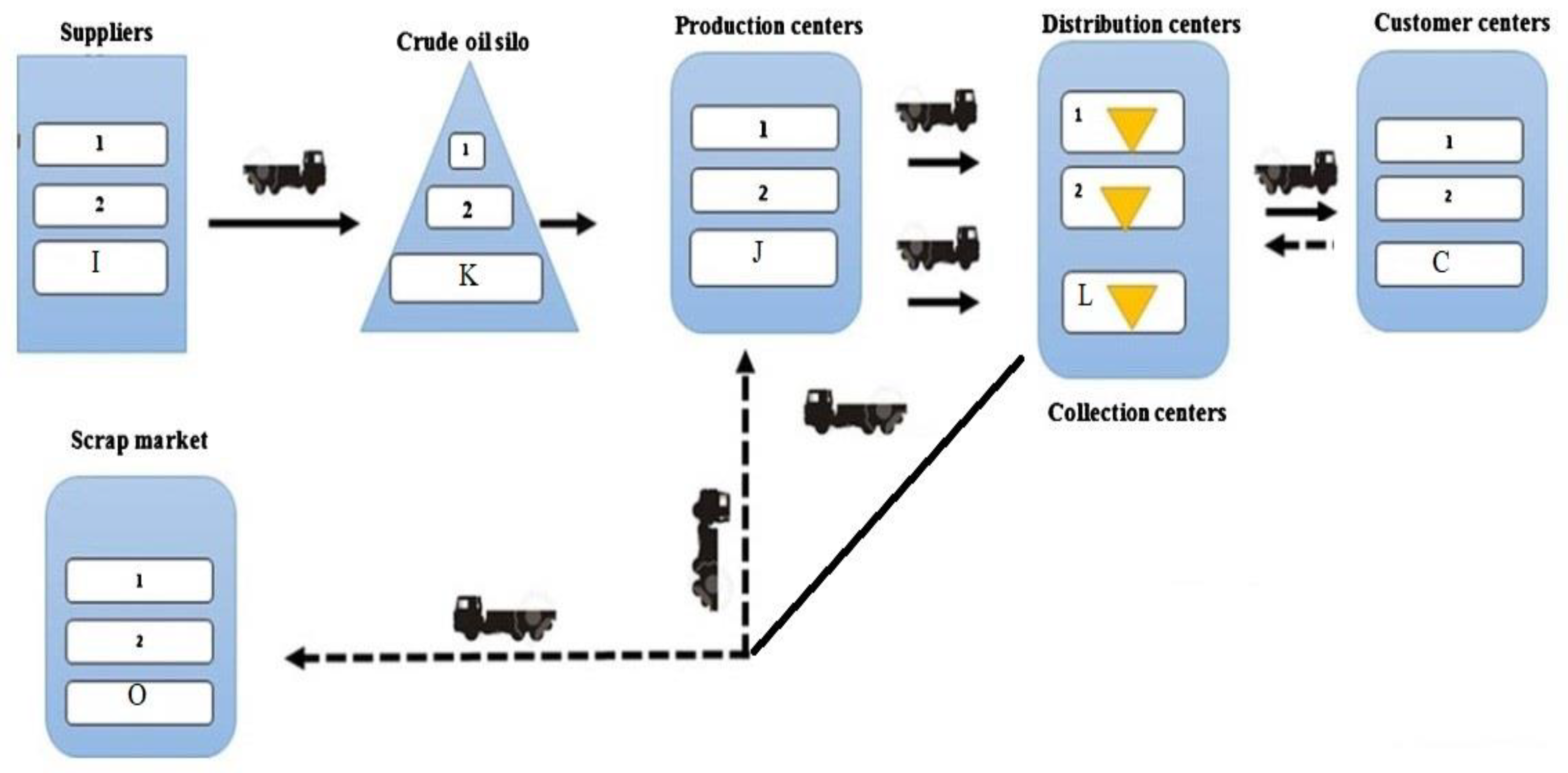
In this section, a CLSC problem is examined. In this model, according to Figure 1, a 7-echelon SCN consisting of raw material suppliers, warehouses (silos), production centers, distribution centers, end customers, collection centers and disposal centers is considered. In this model, customers send their demand for different products to distribution centers. As a result, distribution/collection centers are responsible for the distribution of products and the collection of returned products from customers. This action is performed in the form of vehicle routing. That is, a vehicle collects the returned product at the same time as delivering the product to the customer and transfers it to the collection center. The production centers also produce the products needed by the distribution centers after receiving the raw materials from the warehouse and sending them to that center with different vehicles. Suppliers are also responsible for supplying raw materials and transporting them to warehouses. Moreover, in the reverse SC, after inspection, the collected products are either sent to the production center for reuse or sent to disposal centers for destruction. In addition, due to the limited number of vehicles, a queuing system has been considered in the distribution centers. So that the vehicles wait to receive the cargo in distribution centers. This issue is caused by the presence of uncertain demand in the SCN. Moreover, after receiving the cargo, the vehicles must deliver the products and pick them up within a specific time window. Otherwise, the penalty cost will be added to the objective function (OBF). The main goal of this network is to minimize the costs of the total SCN, including location, allocation and routing. In this problem, the parameters of the problem are considered uncertainty.

In the rest of this section, the definitions of symbols used in modeling are discussed. Due to the existence of uncertainty in the SCN, a non-deterministic model has been designed first. Then the equations related to the M/M/C queuing system in the distribution center have been added to the main model. Finally, the uncertainty parameters have been controlled using the robust-fuzzy-probabilistic method. In this way, each uncertainty parameter is first considered as fuzzy data in different scenarios and then the robust optimization method is used to justify the problem-solving space.

Sets

i Supplier (i = 1,2,…,I)

j Production center (j = 1,2,…,J)

k Candidate locations for crude oil silos (k = 1,2,…,K)

l Candidate locations for distribution/collection center (l = 1,2,…,L)

c Fixed locations of customer (c = 1,2,…,C)

n Collection/distribution centers and customers

(n,n’ = 1,2,…,L,L + 1,…,L + C)

o Fixed locations of disposal center (o = 1,2,…,O)

r Raw materials (crude oil) scrap product (r = 1,2,…,R)

p Final product (p = 1,2,…,P)

t Time period (t = 1,2,…,T)

v Transportation mode (v = 1,2,…,V)

s Scenario (s = 1,2,…,S)

Parameters

$Fix{I}_i$	Supplier selection cost i
$Fix{J}_j$	Production center establishment cost j
$Fix{L}_l$	Distribution/collection center Establishment cost l
$Fix{K}_k$	Warehouse establishment cost k
$Fix{V}_v$	Fixed cost of using the vehicle v
$D_{cpts}$	Product delivery amount p to customer c in period t under scenario s
$R_{cpts}$	Product pick up amount p from customer c in period t under scenario s
$Cap{V}_v$	Vehicle capacity v
$Cap{L}_{lp}$	Maximum distribution center capacity l of product distribution p
$Cap{I}_{ir}$	Maximum supplier capacity i of raw material supply r
$Cap{K}_{kr}$	Maximum storage capacity k of raw material storage r
$Cap{J}_{jp}$	Maximum production center capacity p from the production of product p
$Di{s}_{n{n}^{\prime }}$	Distance between nodes n and n’
$T{r}_{n{n}^{\prime }vs}$	Transportation cost between nodes n and n’ with mode of transport v under scenario s
$T{r}_{ikvs}$	Transportation cost between node i and k with mode of transport v under scenario s
$T{r}_{kjvs}$	Transportation cost between nodes k and j with mode of transport v under scenario s
$T{r}_{jlvs}$	Transportation cost between nodes j and l with mode of transport v under scenario s
$T{r}_{ljvs}$	Transportation cost between nodes l and j with mode of transport v under scenario s
$T{r}_{lovs}$	Transportation cost between node l and o with mode of transport v under scenario s
$T_{n{n}^{\prime }}$	Transportation time between nodes n and n’
$S_c$	Unloading and loading time of the vehicle in the node c
$C_{lp}$	Distribution cost per unit of product p by the distribution center l
$[A{S}_c,B{S}_c]$	Soft time window for pick up delivery of customer products c
$\mathsf{\alpha }$	Penalty cost of soft time window
$\mathrm{H}$	Product-dependent greenhouse gas emissions
$p_s$	Probability of occurrence of scenario s
${\omega }_{rp}$	Number of raw materials r used per unit of product p
$r_p^c$	Average fraction of product recycling p
${\vartheta }_l$	Number of employees in the distribution center l
$C{T}_l$	Waiting time cost to serve in the distribution center l
${\mu }_l$	Distribution center service rate l (exponential distribution)
$B_l$	Upper limit of queue length for service in the distribution center l
${\theta }_l$	High limit probability for excessive service queue length at the distribution center l

Decision variables

$V_{lpvts}$	Product amount total p that can be distributed from the distribution center l by vehicle v under scenario s in period t
$Z_l$	If distribution center l is established/selected, 1 and otherwise 0.
$Z_{lcvts}$	If the distribution center l is assigned to customer c and the vehicle v is assigned under scenario s in period t, 1 and otherwise 0.
$X_{n{n}^{\prime }vts}$	If node n’ is visited after node n by vehicle v under scenario s in period t, 1 and otherwise 0. l, c ∈ L∪C.
$U_{cvts}$	Auxiliary variable for sub-tour deletion limit
$T{c}_{lcvts}$	Vehicle arrives time v at customer c and exits the distribution center l under scenario s in period t
$L{c}_{lcpvts}$	Product amount p in the vehicle load v in the customer node c and out of the distribution center l under scenario s in period t
$T{e}_{cvts}$	Time exceeds the vehicle time window v in customer node c under scenario s in period t
$T{w}_{lvts}$	Maximum vehicle visit time vehicle v out of distribution center l under scenario s in time period t
$Q_{rikvts}^s$	Raw material amount r transferred from the supplier i to the warehouse (silo) k with the transportation mode v in period t under scenario s
$Q_{rkjvts}^h$	Raw material amount r transferred from the warehouse (silo) k to the production center j with the transportation mode v in time period t under scenario s
$Q_{pjlvts}^f$	Product amount p transferred from the production center j to the distribution collection center l with the transportation mode v in period t under scenario s
$Q_{rljvts}^c$	Raw material amount r transferred from the distribution/collection center l to the production center j with the transportation mode v in period t under scenario s
$Q_{rlovts}^d$	Raw material amount/scrap product r transferred from distribution center/collection l to disposal center o with the transportation mode v in period t under scenario s
$y_r^s$	If supplier i is selected to supply raw materials, 1 and otherwise 0.
$y_l^d$	If distribution/collection center l is constructed for product distribution/collection, 1 and otherwise 0.
$y_k^h$	If a warehouse (silo) k is constructed for the storage of raw materials, 1 and otherwise 0.
$y_j^c$	If the production center j is constructed to produce the product, 1 and otherwise 0.

$$\begin{array}{l}Min\omega 1={\displaystyle {\displaystyle \sum }_{l=1}^L}Fix{L}_l{y}_l^d+{\displaystyle {\displaystyle \sum }_{i=1}^I}Fix{I}_i{y}_r^s+{\displaystyle {\displaystyle \sum }_{j=1}^J}Fix{J}_j{y}_j^c+{\displaystyle {\displaystyle \sum }_{k=1}^K}Fix{K}_k{y}_k^h+\\ {\displaystyle {\displaystyle \sum }_{s=1}^S}{P}_s{\displaystyle {\displaystyle \sum }_{n=1}^N{\displaystyle \sum }_{n^{\prime }=1}^N{\displaystyle \sum }_{v=1}^V{\displaystyle \sum }_{t=1}^T}T{r}_{n{n}^{\prime }vs}{X}_{n{n}^{\prime }vts}+{\displaystyle {\displaystyle \sum }_{s=1}^S}{P}_s{\displaystyle {\displaystyle \sum }_{l=1}^L{\displaystyle \sum }_{p=1}^P{\displaystyle \sum }_{v=1}^V{\displaystyle \sum }_{t=1}^T}{C}_{lp}{V}_{lpvts}+\\ {\displaystyle {\displaystyle \sum }_{s=1}^S}{P}_s{\displaystyle {\displaystyle \sum }_{l=1}^L{\displaystyle \sum }_{c=1}^C{\displaystyle \sum }_{v=1}^V{\displaystyle \sum }_{t=1}^T}Fix{V}_v{X}_{lcvts}+{\displaystyle {\displaystyle \sum }_{s=1}^S}{P}_s{\displaystyle {\displaystyle \sum }_{c=1}^C{\displaystyle \sum }_{v=1}^V{\displaystyle \sum }_{t=1}^T}\mathsf{\alpha }T{e}_{cvts} +\\ {\displaystyle {\displaystyle \sum }_{s=1}^S}{P}_s{\displaystyle {\displaystyle \sum }_{i=1}^I{\displaystyle \sum }_{k=1}^K{\displaystyle \sum }_{r=1}^R{\displaystyle \sum }_{v=1}^V{\displaystyle \sum }_{t=1}^T}T{r}_{ikvs}{Q}_{rikvts}^s+\\ {\displaystyle {\displaystyle \sum }_{s=1}^S}{P}_s{\displaystyle {\displaystyle \sum }_{k=1}^K{\displaystyle \sum }_{j=1}^J{\displaystyle \sum }_{r=1}^R{\displaystyle \sum }_{v=1}^V{\displaystyle \sum }_{t=1}^T}T{r}_{kjvs}{Q}_{rkjvts}^h+{\displaystyle {\displaystyle \sum }_{s=1}^S}{P}_s{\displaystyle {\displaystyle \sum }_{j=1}^J{\displaystyle \sum }_{l=1}^L{\displaystyle \sum }_{p=1}^P{\displaystyle \sum }_{v=1}^V{\displaystyle \sum }_{t=1}^T}T{r}_{jlvs}{Q}_{pjlvts}^f\\ +{\displaystyle {\displaystyle \sum }_{s=1}^S}{P}_s{\displaystyle {\displaystyle \sum }_{l=1}^L{\displaystyle \sum }_{j=1}^J{\displaystyle \sum }_{r=1}^R{\displaystyle \sum }_{v=1}^V{\displaystyle \sum }_{t=1}^T}T{r}_{ljvs}{Q}_{rljvts}^c+{\displaystyle {\displaystyle \sum }_{s=1}^S}{P}_s{\displaystyle {\displaystyle \sum }_{l=1}^L{\displaystyle \sum }_{o=1}^O{\displaystyle \sum }_{r=1}^R{\displaystyle \sum }_{v=1}^V{\displaystyle \sum }_{t=1}^T}T{r}_{lovs}{Q}_{rlovts}^d\end{array}$$

(1)

$$Min\omega 2={\displaystyle \sum }_{n=1}^N{\displaystyle \sum }_{n^{\prime }=1}^N{\displaystyle \sum }_{v=1}^V{\displaystyle \sum }_{p=1}^P{\displaystyle \sum }_{v=1}^V{\displaystyle \sum }_{p=1}^P{P}_s.H.Di{s}_{n{n}^{\prime }}L{c}_{n{n}^{\prime }pvts}$$

(2)

$$\begin{gathered} Min\omega 3=max\left\{T{w}_{lvts}\right\} \\ s.t.: \end{gathered}$$

$${\displaystyle \sum }_{v=1}^V{\displaystyle \sum }_{n=1}^N{X}_{lcvts}=1, \forall c,t,s$$

(3)

$${\displaystyle \sum }_{c=1}^C{\displaystyle \sum }_{n=1}^N{\displaystyle \sum }_{p=1}^P{D}_{cpts}{X}_{ncvts}\le Cap{V}_v.F_v, \forall v,t,s$$

(4)

$$U_{cvts}-U_{mvts}+C.X_{cmvts}\le C-1, \forall m,c,v,t,s$$

(5)

$${\displaystyle \sum }_{n=1}^N{X}_{ncvts}={\displaystyle \sum }_{n=1}^N{X}_{cnvts}, \forall v,n,t,s$$

(6)

$${\displaystyle \sum }_{l=1}^L{\displaystyle \sum }_{c=1}^C{X}_{lcvts}\le 1, \forall v,t,s$$

(7)

$$-Z_{lcvts}+{\displaystyle \sum }_{n=1}^N\left(X_{lnvts}+X_{ncvts}\right)\le 1, \forall l,c,v,t,s$$

(8)

$$V_{lpvts}={\displaystyle \sum }_{c=1}^C{D}_{cpts}{Z}_{lcvts}, \forall l,p,v,t,s$$

(9)

$${\displaystyle \sum }_{v=1}^V{V}_{lpvts}\le Cap{L}_{lp}.y_l^d, \forall l,p,t,s$$

(10)

$$L{c}_{lcpvts}\ge V_{lpvts}-D_{cpts}+R_{cpts}-M.\left(1-X_{lcvts}\right), \forall l,p,c,v,t,$$

(11)

$$L{c}_{lmpvts}\ge L{c}_{lcpvts}-D_{mpts}+R_{mpts}-M.\left(1-X_{cmvts}\right), \forall l,p,c,m,v,t,s$$

(12)

$$T{c}_{lcvts}\ge T_{lc}-M.\left(1-X_{lcvts}\right), \forall l,c,v,t,s$$

(13)

$$T{c}_{lmvts}\ge T{c}_{lcvts}+T_{cm}+S_m-M.\left(2-X_{cmvts}-Z_{lcvts}\right), \forall l,c,m,v,t,s$$

(14)

$$T{e}_{cvts}\ge A{S}_c.Z_{lcvts}-T{c}_{lcvts}, \forall l,c,v,t,s$$

(15)

$$T{e}_{cvts}\ge T{c}_{lcvts}-B{S}_c.Z_{lcvts}, \forall l,c,v,t,s$$

(16)

$$T{w}_{lvts}\ge T{c}_{lcvts}+S_c{X}_{clvts}+T_{cl}{X}_{clvts}, \forall l,c,v,t,s$$

(17)

$${\displaystyle \sum }_j{\displaystyle \sum }_v{Q}_{pjlvts}^f={\displaystyle \sum }_v{V}_{lpvts}, \forall l,p,t,s$$

(18)

$${\displaystyle \sum }_k{\displaystyle \sum }_v{Q}_{rkjvts}^h={\displaystyle \sum }_l{\displaystyle \sum }_v{\displaystyle \sum }_p{\omega }_{rp}.Q_{pjlvts}^f, \forall r,j,t,s$$

(19)

$${\displaystyle \sum }_i{\displaystyle \sum }_v{Q}_{rikvts}^s={\displaystyle \sum }_j{\displaystyle \sum }_v{Q}_{rkjvts}^h, \forall r,k,t,s$$

(20)

$$R{e}_{lpvts}\ge L{c}_{lcpvts}-M.\left(2-X_{clvts}-Z_{lcvts}\right), \forall l,c,p,v,t,s$$

(21)

$${\displaystyle \sum }_v{\displaystyle \sum }_p{r}_p^c.R{e}_{lpvt-1s}={\displaystyle \sum }_j{\displaystyle \sum }_v{\displaystyle \sum }_p{\omega }_{rp}.Q_{rljvts}^c, \forall r,l,t,s$$

(22)

$${\displaystyle \sum }_v{\displaystyle \sum }_p\left(1-r_p^c\right).R{e}_{lpvt-1s}={\displaystyle \sum }_o{\displaystyle \sum }_v{\displaystyle \sum }_p{\omega }_{rp}.Q_{rlovts}^d, \forall r,l,t,s$$

(23)

$${\displaystyle \sum }_k{\displaystyle \sum }_v{Q}_{rikvts}^s\le Cap{I}_{ir}.y_r^s, \forall r,i,t,s$$

(24)

$${\displaystyle \sum }_v{\displaystyle \sum }_j{Q}_{rkjwts}^h\le Cap{K}_{kr}.y_k^h, \forall r,k,t,s$$

(25)

$${\displaystyle \sum }_v{\displaystyle \sum }_l{Q}_{pjlvts}^f\le Cap{J}_{jp}.y_j^c, \forall j,p,t,s$$

(26)

$$P\left\{Queue length at the center of distribution l under scenario S in period t>B_l\right\}\le {\theta }_l, \forall l,t,s$$

(27)

$$V_{lpvts},U_{cvts},T{c}_{lcvts},L{c}_{lcpvts},T{e}_{cvts},T{w}_{lvts},Q_{rikvts}^s,Q_{rkjvts}^h,Q_{pjlvts}^f,Q_{rljvts}^c,Q_{rlovts}^d\ge 0$$

(28)

$$Z_l,Z_{lcvts},,y_r^s,y_l^d,y_k^h,y_j^c\in \left\{0,1\right\}$$

(29)

The overall expenses of the CLSC network can be reduced to their lowest possible level using Equation (1). These costs consist of the expenditures associated with the location, transportation and distribution, in addition to the costs associated with going over the allotted time window. The emission of greenhouse gases caused by the transportation of goods is reduced as much as possible by Equation (2). The maximum number of hours that drivers are allowed to work is cut down significantly by Equation (3). Equation (4) provides reassurance that just a single distribution center should be responsible for serving a given consumer. Because of Equation (5), we know that the total quantity of cargo that may be carried by the vehicle cannot exceed its carrying capacity.

In the process of vehicle routing, Equation (6) is known as the sub-tour elimination equation. Equation (7) ensures that every vehicle leaves after visiting a customer by requiring them to do so. Equation (8) ensures that each customer should have only one vehicle assigned to them. Based on Equation (9), it is clear that the vehicle must make its way back to the center after making its rounds to the various clients. The sum of all the products that were dispersed can be found in Equation (10). The solution to Equation (11) ensures that the distribution center can operate at its full capacity in the event that it is constructed. The quantities of merchandise delivered to each consumer by vehicle are shown by Equations (12) and (13), respectively.

The time that the car will arrive to each individual consumer is represented by Equations (14) and (15). The amount of time it takes for each truck to return to the distribution center is represented by Equations (16) and (17). The quantity of commodities that were moved from the production center to the distribution center is represented by Equation (19). It reveals the quantity of raw materials that were moved from the storage facility to the production center in order to facilitate the manufacturing of new goods. The quantity of items that were moved from the supplier to the warehouse is represented by Equation (21). (silo). The quantity of returned commodities in the reverse SC can be calculated using Equation (22). The quantities of commodities that were transported to the collecting center and the destruction facility, respectively, are accounted for by Equations (23) and (24). The limits associated with the capacity of the centers are represented by Equations (25)–(27). The constraint that is related to the length of the line in the middle of the distribution is represented by Equation (28). Equations (29) and (30) demonstrate the variables involved in decision making.

3.1. Jackson Network

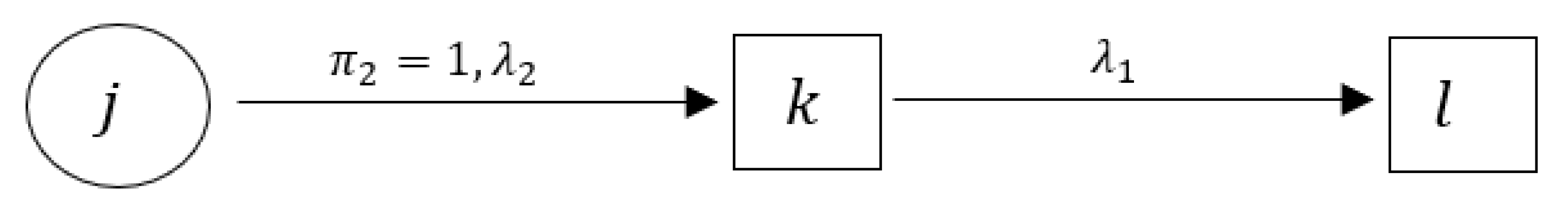
In the SCN, goods are usually sent from distribution centers where parallel service providers are responsible for packing, loading, etc. The existence of different demands from customers makes it difficult to manage the distribution of goods. Therefore, a queue system is usually created in the distribution centers. Determining the number of servers can reduce the queue length while it can change the overall SCN costs. Therefore, in the optimization of SCN problems, it is very important to consider the queuing system in order to reduce costs and reduce queue length. The distribution centers chosen for research in Figure 2 of the Jackson network and the suggested network equations are presented below [67]:

$${\pi }_2{\lambda }_2={\lambda }_1$$

(30)

In above the Equation, ${\lambda }_1$ and ${\lambda }_2$ are input rates and ${\pi }_2$ is the output rate for k center. Therefore, according to the values mentioned in the figure, the input rate to the distribution center is obtained as follows:

$${\lambda }_2={\lambda }_1$$

(31)

As a result, in the designed SCN, the queuing system in the distribution center is considered, whose entry rate includes the number of products sent from the production center for distribution to customers, and its exit rate is equal to all the products that are being is distributed. Therefore, due to uncertain demand, a queue system is formed as follows:

$${\lambda }_{lts}={\displaystyle \sum }_{p=1}^P{\displaystyle \sum }_{j=1}^J{\displaystyle \sum }_{v=1}^V{Q}_{pjlvts}^f, \forall l,t,s$$

(32)

The model must be changed to a specific condition in order to satisfy Equation (28); therefore, this constraint is changed to a definite constraint using an M/M/C queue model. The input rate equal to λ (Poisson distribution) and the service time are used in this model to construct the M/M/C queue for the distribution center μ (exponential distribution). There are m servers with a constrained capacity C in the queue model.

$${\displaystyle \sum }_{k^{\prime }={\vartheta }_l+B_l+1}^C{P}_{l^{\prime }lts}\le {\theta }_l or 1-{\displaystyle \sum }_{l^{\prime }=0}^{{\vartheta }_l+B_l}{P}_{l^{\prime }lts}\le {\theta }_l, \forall l,t,s$$

(33)

The first expression of Equation (34) shows that the likelihood that there are fewer than n customers in the service queue of the distribution center l with ${\vartheta }_l$ of the server is less than ${\theta }_l$, and the second equation demonstrates that the total of all probabilities is equivalent to 1. The rate of service may be derived by doing the following:

$${\mu }_{nl}=\{\begin{array}{c}\begin{array}{cc}n{\mu }_l& n\le {\vartheta }_l\end{array}\\ \begin{array}{cc}{\vartheta }_l{\mu }_l& {\vartheta }_l<n<C\end{array}\end{array}, \forall l$$

(34)

By combining the above constraints ${\pi }_{0lts}$ (the probability of selecting a node as the distribution center l under scenario s in period t) is obtained as follows:

$${\pi }_{0lts}={\left[{\displaystyle \sum }_{l^{\prime }=0}^{{\vartheta }_l - 1}\frac{1}{l^{\prime }!}{\left(\frac{{\lambda }_{lts}}{{\mu }_l}\right)}^{l^{\prime }} + \frac{1}{{\vartheta }_l!}{\left(\frac{{\lambda }_{lts}}{{\mu }_l}\right)}^{{\vartheta }_l}\left(\frac{{\vartheta }_l{\mu }_l}{{\vartheta }_l{\mu }_l - {\lambda }_{lts}}\right)\right]}^{-1}, \forall l,t,s$$

(35)

In the results, the probability of a robust condition for n customers in the service queue of distribution center l (Equation (28)) is as follows [67,68]:

$$P_{nlts}=\{\begin{array}{c}\begin{array}{cc}\frac{{\lambda }_{lts}^n}{n!{\mu }_l^n}{\pi }_{0lts}& 1\le n\le {\vartheta }_l\end{array}\\ \begin{array}{cc}\frac{{\lambda }_{lts}^n{\vartheta }_l{}^{n-{\vartheta }_l}}{n!{\mu }_l^n}{\pi }_{0lts}& {\vartheta }_l<n\le C\end{array}\end{array} \forall l,t,s$$

(36)

$$P_{l^{\prime }lt}={\displaystyle \sum }_{l^{\prime }=0}^{{\vartheta }_l}\frac{{\lambda }_{lts}^{l^{\prime }}}{l^{\prime }!{\mu }_l^{l^{\prime }}}{\pi }_{0lts}+{\displaystyle \sum }_{l^{\prime }={\vartheta }_l+1}^{{\vartheta }_l+B_l}\frac{{\lambda }_{lts}^{l^{\prime }}{\vartheta }_l{}^{l^{\prime }-{\vartheta }_l}}{l^{\prime }!{\mu }_l^{l^{\prime }}}{\pi }_{0lts}\ge 1-{\theta }_l, \forall l,t,s$$

(37)

$$P_{l^{\prime }lts}=\left({\displaystyle \sum }_{l^{\prime }=0}^{{\vartheta }_l}\frac{{\lambda }_{lts}^{l^{\prime }}}{l^{\prime }!{\mu }_l^{l^{\prime }}}+{\displaystyle \sum }_{l^{\prime }={\vartheta }_l+1}^{{\vartheta }_l+B_l}\frac{{\lambda }_{lts}^{l^{\prime }}{\vartheta }_l{}^{l^{\prime }-{\vartheta }_l}}{l^{\prime }!{\mu }_l^{l^{\prime }}}\right){\pi }_{0lts}\ge 1-{\theta }_l, \forall l,t,s$$

(38)

Moreover, according to the above, the customer waiting time in the l distribution center can be obtained, as described in Equation (39) as follows:

$$W_{lts}=\left[\frac{{\pi }_{0lts}}{{\vartheta }_l!}{\left(\frac{{\lambda }_{lts}}{{\mu }_l}\right)}^{{\vartheta }_l!}\frac{{\vartheta }_l{\mu }_l}{{\left({\vartheta }_l{\mu }_l - {\lambda }_{lts}\right)}^2} + \frac{1}{{\mu }_l}\right]y_l^d, \forall l,t,s$$

(39)

The amount of customer waiting time cost in the distribution center l, ${{\displaystyle \sum }}_{l=1}^L{{\displaystyle \sum }}_{t=1}^T{{\displaystyle \sum }}_{s=1}^S{P}_s.W_{lts}.C{T}_l$ is also added to the first OBF as an additional cost.

3.2. Robust-Fuzzy-Probabilistic Method

Because of the unpredictable nature of a number of important factors (such as the costs of transportation and demand), which are not amenable to planning, as well as the unavailability and even the unavailability of historical data that is necessary during the design stage, these characteristics are largely dependent on points of view. Since the mental experiences of experts are also approximated, the previously described hazy parameters are given as uncertain data in the form of trapezoidal fuzzy numbers. It is essential to keep in mind that calculating the production facility’s capacity, demand and transportation costs for long-term decisions may be difficult, if not impossible. This is why it is crucial to keep this in mind. Even if it is possible to estimate a distribution function for these parameters, it is possible that they will not behave in the same manner as the data from earlier times. As a consequence of this, the data obtained from these variables, which change over an extended period of time, are considered to be fuzzy [69].

Furthermore, uncertain (probable) restrictions are often handled using indefinite finite programming where uncertain data on the left or right side is equal. The notion of decision-making may accomplish the lowest degree of certainty as an acceptable safe margin for imposing any of these restrictions if this approach is utilized to regulate the confidence level in generating these indefinite limits. Two regularly used standard fuzzy method actions, with optimistic fuzzy and pessimistic fuzzy names, are utilized to accomplish this. It is noteworthy that the pessimistic fuzzy represents the pessimistic choice of the uncertain event, while the optimistic fuzzy reflects the degree of optimistic probability of the occurrence of an uncertain event, including unknown parameters. We presume that decision-making has a pessimistic and optimistic attitude while concurrently imposing indefinite limits; thus, we utilize a pessimistic-optimistic combination fuzzy; this is more cautious. Currently, the obvious counterpart of the original indefinite model can be stated using the ambiguous parameters mentioned above, the anticipated value for the OBF and the pessimistic-optimistic action for the indefinite constraints. To start, think about the model’s condensed version given in [70] as follows:

$$\begin{gathered} min\mathrm{Z}=F.y+{\tilde{C}}_s.x_s \\ s.t.: \\ A{x}_s\ge {\tilde{D}}_s \\ Bx<\mathrm{S}y \\ y\in \left\{0,1\right\},x_s\ge 0 \end{gathered}$$

(40)

${\tilde{D}}_s$, ${\tilde{C}}_s$, F and $s$ indicate the fixed cost of construction, variable cost (transportation), demand and facility capacity, respectively. A and E are coefficient matrices, while $x_s$ and $y$ are continuous variables, zero and one for scenario s. In the given model, the vectors ${\tilde{D}}_s$ and ${\tilde{C}}_s$ are indeterminate parameters. The general form of uncertain restricted planning requires the anticipated value of the OBF and the pessimistic fuzzy to handle the OBF and indefinite constraint, respectively. The acronym’s pessimistic fuzzy basic model is as follows:

$$\begin{gathered} minZ=E\left[Z\right]=F.y+E\left[{\tilde{C}}_s\right].x_s \\ s.t.: \\ NEC\left\{A{x}_s\ge {\tilde{D}}_s\right\}\ge {\alpha }_s \\ Bx<\mathrm{S}y \\ y\in \left\{0,1\right\},x_s\ge 0 \end{gathered}$$

(41)

where ${\alpha }_s$ (pessimistic) decision-making controls the lowest degree of confidence of uncertain constraint. Equation (42) is given by the trapezoidal probability distribution for the following conditions [69]:

$$\begin{gathered} minZ=F.y+\left(\frac{{\mathrm{C}}_s^1+{\mathrm{C}}_s^2+{\mathrm{C}}_s^3+{\mathrm{C}}_s^4}{4}\right)x_s \\ s.t.: \\ A{x}_s\ge \left(1-{\alpha }_s\right)D_s^3+{\alpha }_s{D}_s^4 \\ Bx<Sy \\ y\in \left\{0,1\right\},x_s\ge 0 \end{gathered}$$

(42)

Moreover, the general form of Uncertain limited planning, OBF expected value and the optimistic fuzzy to deal with the OBF and the uncertain constraint, respectively, are as follows:

$$\begin{gathered} minZ=E\left[\mathrm{Z}\right]=F.y+\mathrm{E}\left[{\tilde{C}}_s\right].x_s \\ s.t.: \\ POS\left\{A{x}_s\ge {\tilde{D}}_s\right\}\ge {\alpha }_s \\ Bx<Sy \\ y\in \left\{0,1\right\},x_s\ge 0 \end{gathered}$$

(43)

The optimistic fuzzy’s pessimistic controls the indefinite constraint’s minimal degree of confidence. Equation (44) is given by the trapezoidal probability distribution for ambiguous parameters as follows [59]:

$$\begin{gathered} minZ=F.y+\left(\frac{{\mathrm{C}}_s^1+{\mathrm{C}}_s^2+{\mathrm{C}}_s^3+{\mathrm{C}}_s^4}{4}\right)x_s \\ s.t.: \\ A{x}_s\ge \left(1-{\alpha }_s\right)D_s^1+{\alpha }_s{D}_s^2 \\ Bx<Sy \\ y\in \left\{0,1\right\},x_s\ge 0 \end{gathered}$$

(44)

According to the relationships expressed in this paper, a new pessimistic-optimistic fuzzy hybrid model has been used to control uncertain parameters. Therefore, the pessimistic-optimistic fuzzy base model is as follows:

$$\begin{gathered} minZ=E\left[\mathrm{Z}\right]=F.y+\mathrm{E}\left[{\tilde{C}}_s\right].x_s \\ s.t.: \\ \left(1-{\nu }_1\right)\left[NEC\left\{A{x}_s\ge {\tilde{D}}_s\right\}\ge {\alpha }_s\right]+\left({\nu }_1\right)\left[POS\left\{A{x}_s\ge {\tilde{D}}_s\right\}\ge {\alpha }_s\right] \\ Bx<Sy \\ y\in \left\{0,1\right\},x\ge 0 \end{gathered}$$

(45)

In the pessimistic-optimistic fuzzy basic model and Equation (46), ${\nu }_1$ is parameter zero and one; If ${\nu }_1$ takes 1, the hybrid fuzzy model becomes an optimistic fuzzy model and if ${\nu }_1$ takes 0, the hybrid fuzzy model becomes a pessimistic fuzzy model. Moreover, if ${\nu }_1$ takes the value 0.5, the combined fuzzy model becomes the moderate fuzzy model, so to solve the final model in this paper, ${\nu }_1$ will be defined as parameters with three values 0, 0.5 and 1. Finally, the main model for controlling uncertain parameters in hybrid fuzzy is as follows [71]:

$$\begin{gathered} minZ=F.y+\left(\frac{C_s^1+C_s^2+C_s^3+C_s^4}{4}\right)x_s \\ s.t.: \\ A{x}_s\ge \left(1-{\nu }_1\right)\left[\left(1-{\alpha }_s\right)D_s^3+{\alpha }_s{D}_s^4\right]+\left({\nu }_1\right)\left[\left(1-{\alpha }_s\right)D_s^1+{\alpha }_s{D}_s^2\right] \\ Bx<Sy \\ y,\in \left\{0,1\right\},x_s\ge 0,{\alpha }_s,{\beta }_s\in \left[0.5,1\right] \end{gathered}$$

(46)

Decision preferences establish the lowest confidence level for unknown constraints in probabilistic models. The OBF in the suggested models is not sensitive to variation from its predicted value; hence, robust solutions in the base model are not guaranteed. In such instances, the excessive risk may affect decision-making in many practical scenarios, particularly strategic ones when solution consolidation is most important. To address this inefficiency, robust-stochastic uncertain planning is utilized. Robust and stochastic planning make this uncertainty planning technique stand out. The following suggested model is used for uncertainty planning in this study:

$$\begin{gathered} min{\omega }_1=E\left[\mathrm{Z}\right]+\xi \left(Z_{\left(max\right)}-Z_{\left(min\right)}\right)+\omega {\displaystyle \sum }_s{P}_s\left\{E\left[Z\right]-E\left[Z_s\right]+2{\theta }_s\right\} \\ {\eta }_1{\displaystyle \sum }_s{P}_s\left[D_s^4-\frac{\left({\alpha }_s-\lambda \right)D_s^4+\left(1-{\alpha }_s\right)D_s^3}{1-\lambda }\right] \\ s.t.: \\ A{x}_s\ge \left(1-{\nu }_1\right)\left[\left(1-{\alpha }_s\right)D_s^3+{\alpha }_s{D}_s^4\right]+\left({\nu }_1\right)\left[\left(1-{\alpha }_s\right)D_s^1+{\alpha }_s{D}_s^2\right] \\ Bx<Sy \\ y,\in \left\{0,1\right\},x_s\ge 0,{\alpha }_s,{\beta }_s\in \left[0.5,1\right] \end{gathered}$$

(47)

where M is a huge non-negative number and $Z_{\left(max\right)}$, $Z_{\left(min\right)}$ and $E\left[Z_s\right]$ can be expressed as follows:

$$\begin{gathered} Z_{\left(max\right)}=F.y+{\displaystyle \sum }_s{P}_s{C}_s^4{x}_s \\ {Z}_{\left(min\right)}=F.y+{\displaystyle \sum }_s{P}_s{C}_s^1{x}_s \\ E\left[Z_s\right]=F.y+\left[\frac{1-\lambda }{2}\left(C_s^1+C_s^2\right)+\frac{\lambda }{2}\left(C_s^3+C_s^4\right)\right].x_s \end{gathered}$$

(48)

The first equation in Equation (48)’s first OBF is the expected value using the model’s mean uncertain parameters. The cost of the penalty for deviating from the anticipated value of the first OBF is the second statement. The third phrase displays the overall demand deviation penalty cost (uncertain parameter). Thus, the OBF weight coefficient is $\xi$, and ${\eta }_1$ the penalty for not predicting demand is 1. The coefficients of correction in fuzzy number surfaces should be between 0.5 and 1. The queuing system-controlled SCN model is [72].

$$\begin{array}{l}Min\omega 1=E\left[Z\right]+\xi \left(Zmax-Zmin\right)+\omega {\displaystyle {\displaystyle \sum }_s}{P}_s\left\{E\left[Z\right]-E\left[Z_s\right]+2{\theta }_s\right\}\\ +{\eta }_1{\displaystyle {\displaystyle \sum }_c{\displaystyle \sum }_p{\displaystyle \sum }_t{\displaystyle \sum }_s}{P}_s\left[D_{cpts}^4-\frac{\left({\alpha }_s-\mathsf{\psi }\right)D_{cpts}^4+\left(1-{\alpha }_s\right)D_{cpts}^3}{1-\lambda }\right]\\ +{\eta }_2{\displaystyle {\displaystyle \sum }_c{\displaystyle \sum }_p{\displaystyle \sum }_t{\displaystyle \sum }_s}{P}_s\left[R_{cpts}^4-\frac{\left({\alpha }_s-\mathsf{\psi }\right)R_{cpts}^4+\left(1-{\alpha }_s\right)R_{cpts}^3}{1-\lambda }\right]\end{array}$$

(49)

$$Min\omega 2={\displaystyle \sum }_{n=1}^N{\displaystyle \sum }_{n^{\prime }=1}^N{\displaystyle \sum }_{v=1}^V{\displaystyle \sum }_{p=1}^P{\displaystyle \sum }_{v=1}^V{\displaystyle \sum }_{p=1}^P{P}_s.H.Di{s}_{n{n}^{\prime }}L{c}_{n{n}^{\prime }pvts}$$

(50)

$$Min\omega 3=max\left\{T{w}_{lvts}\right\}$$

(51)

$$s.t.:$$

$${\displaystyle \sum }_{v=1}^V{\displaystyle \sum }_{n=1}^N{X}_{lcvts}=1,\forall c,t,s$$

(52)

$$\begin{gathered} {\displaystyle \sum }_{c=1}^C{\displaystyle \sum }_{n=1}^N{\displaystyle \sum }_{p=1}^P\left[\left(1-{\nu }_1\right)\left[\left(1-{\alpha }_s\right)D_{cpts}^3+{\alpha }_s{D}_{cpts}^4\right]+\left({\nu }_1\right)\left[\left(1-{\alpha }_s\right)D_{cpts}^1+{\alpha }_s{D}_{cpts}^2\right]\right]X_{ncvts} \\ \le Cap{V}_v.F_v,\forall v,t,s \end{gathered}$$

(53)

$$U_{cvts}-U_{mvts}+C.X_{cmvts}\le C-1,\forall m,c,v,t,s$$

(54)

$${\displaystyle \sum }_{n=1}^N{X}_{ncvts}={\displaystyle \sum }_{n=1}^N{X}_{cnvts},\forall v,n,t,s$$

(55)

$${\displaystyle \sum }_{l=1}^L{\displaystyle \sum }_{c=1}^C{X}_{lcvts}\le 1,\forall v,t,s$$

(56)

$$-Z_{lcvts}+{\displaystyle \sum }_{n=1}^N\left(X_{lnvts}+X_{ncvts}\right)\le 1,\forall l,c,v,t,s$$

(57)

$$V_{lpvts}={\displaystyle \sum }_{c=1}^C\left[\left(1-{\nu }_1\right)\left[\left(1-{\alpha }_s\right)D_{cpts}^3+{\alpha }_s{D}_{cpts}^4\right]+\left({\nu }_1\right)\left[\left(1-{\alpha }_s\right)D_{cpts}^1+{\alpha }_s{D}_{cpts}^2\right]\right]Z_{lcvts},\forall l,p,v,t,s$$

(58)

$${\displaystyle \sum }_{v=1}^V{V}_{lpvts}\le Cap{L}_{lp}.y_l^d,\forall l,p,t,s$$

(59)

$$\begin{array}{l}{Lc}_{lcpvts}\ge V_{lpvts}-\left[\left(1-{\nu }_1\right)\left[\left(1-{\alpha }_s\right)D_{cpts}^3+{\alpha }_s{D}_{cpts}^4\right]+\left({\nu }_1\right)\left[\left(1-{\alpha }_s\right)D_{cpts}^1+{\alpha }_s{D}_{cpts}^2\right]\right]\\ \hspace{1em}\hspace{1em}\hspace{1em}\hspace{1em}\hspace{1em} +\left[\left(1-{\nu }_1\right)\left[\left(1-{\alpha }_s\right)R_{cpts}^3+{\alpha }_s{R}_{cpts}^4\right]+\left({\nu }_1\right)\left[\left(1-{\alpha }_s\right)R_{cpts}^1+{\alpha }_s{R}_{cpts}^2\right]\right]\\ \hspace{1em}\hspace{1em}\hspace{1em}\hspace{1em}\hspace{1em} -M.\left(1-X_{lcvts}\right),\forall l,p,c,v,t,\end{array}$$

(60)

$$\begin{array}{l}{Lc}_{lmpvts}\ge {Lc}_{lcpvts}-\left[\left(1-{\nu }_1\right)\left[\left(1-{\alpha }_s\right)D_{cpts}^3+{\alpha }_s{D}_{cpts}^4\right]+\left({\nu }_1\right)\left[\left(1-{\alpha }_s\right)D_{cpts}^1+{\alpha }_s{D}_{cpts}^2\right]\right]\\ \hspace{1em}\hspace{1em}\hspace{1em}\hspace{1em}\hspace{1em}+\left[\left(1-{\nu }_1\right)\left[\left(1-{\alpha }_s\right)R_{cpts}^3+{\alpha }_s{R}_{cpts}^4\right]+\left({\nu }_1\right)\left[\left(1-{\alpha }_s\right)R_{cpts}^1+{\alpha }_s{R}_{cpts}^2\right]\right]\\ \hspace{1em}\hspace{1em}\hspace{1em}\hspace{1em}\hspace{1em}-M.\left(1-X_{cmvts}\right),\forall l,p,c,m,v,t,s\end{array}$$

(61)

$$T{c}_{lcvts}\ge T_{lc}-M.\left(1-X_{lcvts}\right),\forall l,c,v,t,s$$

(62)

$$T{c}_{lmvts}\ge T{c}_{lcvts}+T_{cm}+S_m-M.\left(2-X_{cmvts}-Z_{lcvts}\right),\forall l,c,m,v,t,s$$

(63)

$$T{e}_{cvts}\ge A{S}_c.Z_{lcvts}-T{c}_{lcvts},\forall l,c,v,t,s$$

(64)

$$T{e}_{cvts}\ge T{c}_{lcvts}-B{S}_c.Z_{lcvts},\forall l,c,v,t,s$$

(65)

$$T{w}_{lvts}\ge T{c}_{lcvts}+S_c{X}_{clvts}+T_{cl}{X}_{clvts},\forall l,c,v,t,s$$

(66)

$${\displaystyle \sum }_j{\displaystyle \sum }_v{Q}_{pjlvts}^f={\displaystyle \sum }_v{V}_{lpvts},\forall l,p,t,s$$

(67)

$${\displaystyle \sum }_k{\displaystyle \sum }_v{Q}_{rkjvts}^h={\displaystyle \sum }_l{\displaystyle \sum }_v{\displaystyle \sum }_p{\omega }_{rp}.Q_{pjlvts}^f,\forall r,j,t,s$$

(68)

$${\displaystyle \sum }_i{\displaystyle \sum }_v{Q}_{rikvts}^s={\displaystyle \sum }_j{\displaystyle \sum }_v{Q}_{rkjvts}^h,\forall r,k,t,s$$

(69)

$$R{e}_{lpvts}\ge L{c}_{lcpvts}-M.\left(2-X_{clvts}-Z_{lcvts}\right),\forall l,c,p,v,t,s$$

(70)

$${\displaystyle \sum }_v{\displaystyle \sum }_p{r}_p^c.R{e}_{lpvt-1s}={\displaystyle \sum }_j{\displaystyle \sum }_v{\displaystyle \sum }_p{\omega }_{rp}.Q_{rljvts}^c,\forall r,l,t,s$$

(71)

$${\displaystyle \sum }_v{\displaystyle \sum }_p\left(1-r_p^c\right).R{e}_{lpvt-1s}={\displaystyle \sum }_o{\displaystyle \sum }_v{\displaystyle \sum }_p{\omega }_{rp}.Q_{rlovts}^d,\forall r,l,t,s$$

(72)

$${\displaystyle \sum }_k{\displaystyle \sum }_v{Q}_{rikvts}^s\le Cap{I}_{ir}.y_r^s,\forall r,i,t,s$$

(73)

$${\displaystyle \sum }_v{\displaystyle \sum }_j{Q}_{rkjwts}^h\le Cap{K}_{kr}.y_k^h,\forall r,k,t,s$$

(74)

$${\displaystyle \sum }_v{\displaystyle \sum }_l{Q}_{pjlvts}^f\le Cap{J}_{jp}.y_j^c,\forall j,p,t,s$$

(75)

$${\lambda }_{lts}={\displaystyle \sum }_{p=1}^P{\displaystyle \sum }_{j=1}^J{\displaystyle \sum }_{v=1}^V{Q}_{pjlvts}^f,\forall l,t,s$$

(76)

$$W_{lts}=\left[\frac{{\pi }_{0lts}}{{\vartheta }_l!}{\left(\frac{{\lambda }_{lts}}{{\mu }_l}\right)}^{{\vartheta }_l!}\frac{{\vartheta }_l{\mu }_l}{{\left({\vartheta }_l{\mu }_l-{\lambda }_{lts}\right)}^2}+\frac{1}{{\mu }_l}\right]y_l^d,\forall l,t,s$$

(77)

$${\pi }_{0lts}={\left[{\displaystyle \sum }_{l^{\prime }=0}^{{\vartheta }_l-1}\frac{1}{l^{\prime }!}{\left(\frac{{\lambda }_{lts}}{{\mu }_l}\right)}^{l^{\prime }}+\frac{1}{{\vartheta }_l!}{\left(\frac{{\lambda }_{lts}}{{\mu }_l}\right)}^{{\vartheta }_l}\left(\frac{{\vartheta }_l{\mu }_l}{{\vartheta }_l{\mu }_l-{\lambda }_{lts}}\right)\right]}^{-1},\forall l,t,s$$

(78)

$$\left({\displaystyle \sum }_{l^{\prime }=0}^{{\vartheta }_l}\frac{{\lambda }_{lts}^{l^{\prime }}}{l^{\prime }!{\mu }_l^{l^{\prime }}}+{\displaystyle \sum }_{l^{\prime }={\vartheta }_l+1}^{{\vartheta }_l+B_l}\frac{{\lambda }_{lts}^{l^{\prime }}{\vartheta }_l{}^{l^{\prime }-{\vartheta }_l}}{l^{\prime }!{\mu }_l^{l^{\prime }}}\right){\pi }_{0lts}\ge 1-{\theta }_l,\forall l,t,s$$

(79)

$$\begin{array}{l}Zmin={\displaystyle {\displaystyle \sum }_{l=1}^L}Fix{L}_l{y}_l^d+{\displaystyle {\displaystyle \sum }_{i=1}^I}Fix{I}_i{y}_r^s+{\displaystyle {\displaystyle \sum }_{j=1}^J}Fix{J}_j{y}_j^c+{\displaystyle {\displaystyle \sum }_{k=1}^K}Fix{K}_k{y}_k^h+\\ {\displaystyle {\displaystyle \sum }_{s=1}^S}{P}_s{\displaystyle {\displaystyle \sum }_{n=1}^N{\displaystyle \sum }_{n^{\prime }=1}^N{\displaystyle \sum }_{v=1}^V{\displaystyle \sum }_{t=1}^T}T{r}_{n{n}^{\prime }vs}^1{X}_{n{n}^{\prime }vts}+{\displaystyle {\displaystyle \sum }_{s=1}^S}{P}_s{\displaystyle {\displaystyle \sum }_{l=1}^L{\displaystyle \sum }_{p=1}^P{\displaystyle \sum }_{v=1}^V{\displaystyle \sum }_{t=1}^T}{C}_{lp}{V}_{lpvts}+\\ {\displaystyle {\displaystyle \sum }_{s=1}^S}{P}_s{\displaystyle {\displaystyle \sum }_{l=1}^L{\displaystyle \sum }_{c=1}^C{\displaystyle \sum }_{v=1}^V{\displaystyle \sum }_{t=1}^T}Fix{V}_v{X}_{lcvts}+{\displaystyle {\displaystyle \sum }_{s=1}^S}{P}_s{\displaystyle {\displaystyle \sum }_{c=1}^C{\displaystyle \sum }_{v=1}^V{\displaystyle \sum }_{t=1}^T}\mathsf{\alpha }T{e}_{cvts}+\\ {\displaystyle {\displaystyle \sum }_{s=1}^S}{P}_s{\displaystyle {\displaystyle \sum }_{i=1}^I{\displaystyle \sum }_{k=1}^K{\displaystyle \sum }_{r=1}^R{\displaystyle \sum }_{v=1}^V{\displaystyle \sum }_{t=1}^T}T{r}_{ikvs}^1{Q}_{rikvts}^s+{\displaystyle {\displaystyle \sum }_{s=1}^S}{P}_s{\displaystyle {\displaystyle \sum }_{l=1}^L{\displaystyle \sum }_{o=1}^O{\displaystyle \sum }_{r=1}^R{\displaystyle \sum }_{v=1}^V{\displaystyle \sum }_{t=1}^T}T{r}_{lovs}^1{Q}_{rlovts}^d+\\ {\displaystyle {\displaystyle \sum }_{s=1}^S}{P}_s{\displaystyle {\displaystyle \sum }_{k=1}^K{\displaystyle \sum }_{j=1}^J{\displaystyle \sum }_{r=1}^R{\displaystyle \sum }_{v=1}^V{\displaystyle \sum }_{t=1}^T}T{r}_{kjvs}^1{Q}_{rkjvts}^h+{\displaystyle {\displaystyle \sum }_{s=1}^S}{P}_s{\displaystyle {\displaystyle \sum }_{j=1}^J{\displaystyle \sum }_{l=1}^L{\displaystyle \sum }_{p=1}^P{\displaystyle \sum }_{v=1}^V{\displaystyle \sum }_{t=1}^T}T{r}_{jlvs}^1{Q}_{pjlvts}^f\\ +{\displaystyle {\displaystyle \sum }_{s=1}^S}{P}_s{\displaystyle {\displaystyle \sum }_{l=1}^L{\displaystyle \sum }_{j=1}^J{\displaystyle \sum }_{r=1}^R{\displaystyle \sum }_{v=1}^V{\displaystyle \sum }_{t=1}^T}T{r}_{ijvs}^1{Q}_{rljvts}^c+{\displaystyle {\displaystyle \sum }_{l=1}^L{\displaystyle \sum }_{t=1}^T{\displaystyle \sum }_{s=1}^S}{P}_s.W_{lts}.C{T}_l\end{array}$$

(80)

$$\begin{array}{l}Zmax={\displaystyle {\displaystyle \sum }_{l=1}^L}Fix{L}_l{y}_l^d+{\displaystyle {\displaystyle \sum }_{i=1}^I}Fix{I}_i{y}_r^s+{\displaystyle {\displaystyle \sum }_{j=1}^J}Fix{J}_j{y}_j^c+{\displaystyle {\displaystyle \sum }_{k=1}^K}Fix{K}_k{y}_k^h+\\ {\displaystyle {\displaystyle \sum }_{s=1}^S}{P}_s{\displaystyle {\displaystyle \sum }_{n=1}^N{\displaystyle \sum }_{n^{\prime }=1}^N{\displaystyle \sum }_{v=1}^V{\displaystyle \sum }_{t=1}^T}T{r}_{n{n}^{\prime }vs}^1{X}_{n{n}^{\prime }vts}+{\displaystyle {\displaystyle \sum }_{s=1}^S}{P}_s{\displaystyle {\displaystyle \sum }_{l=1}^L{\displaystyle \sum }_{p=1}^P{\displaystyle \sum }_{v=1}^V{\displaystyle \sum }_{t=1}^T}{C}_{lp}{V}_{lpvts}+\\ {\displaystyle {\displaystyle \sum }_{s=1}^S}{P}_s{\displaystyle {\displaystyle \sum }_{l=1}^L{\displaystyle \sum }_{c=1}^C{\displaystyle \sum }_{v=1}^V{\displaystyle \sum }_{t=1}^T}Fix{V}_v{X}_{lcvts}+{\displaystyle {\displaystyle \sum }_{s=1}^S{P}_s{\displaystyle \sum }_{c=1}^C{\displaystyle \sum }_{v=1}^V{\displaystyle \sum }_{t=1}^T}\mathsf{\alpha }T{e}_{cvts}+\\ {\displaystyle {\displaystyle \sum }_{s=1}^S}{P}_s{\displaystyle {\displaystyle \sum }_{i=1}^I{\displaystyle \sum }_{k=1}^K{\displaystyle \sum }_{r=1}^R{\displaystyle \sum }_{v=1}^V{\displaystyle \sum }_{t=1}^T}T{r}_{ikvs}^4{Q}_{rikvts}^s+{\displaystyle {\displaystyle \sum }_{s=1}^S{P}_s{\displaystyle \sum }_{l=1}^L{\displaystyle \sum }_{o=1}^O{\displaystyle \sum }_{r=1}^R{\displaystyle \sum }_{v=1}^V{\displaystyle \sum }_{t=1}^T}T{r}_{lovs}^4{Q}_{rlovts}^d+\\ {\displaystyle {\displaystyle \sum }_{s=1}^S}{P}_s{\displaystyle {\displaystyle \sum }_{k=1}^K{\displaystyle \sum }_{j=1}^J{\displaystyle \sum }_{r=1}^R{\displaystyle \sum }_{v=1}^V{\displaystyle \sum }_{t=1}^T}T{r}_{kjvs}^4{Q}_{rkjvts}^h+{\displaystyle {\displaystyle \sum }_{s=1}^S{P}_s{\displaystyle \sum }_{j=1}^J{\displaystyle \sum }_{l=1}^L{\displaystyle \sum }_{p=1}^P{\displaystyle \sum }_{v=1}^V{\displaystyle \sum }_{t=1}^T}T{r}_{jlvs}^4{Q}_{pjlvts}^f\\ +{\displaystyle {\displaystyle \sum }_{s=1}^S}{P}_s{\displaystyle {\displaystyle \sum }_{l=1}^L{\displaystyle \sum }_{j=1}^J{\displaystyle \sum }_{r=1}^R{\displaystyle \sum }_{v=1}^V{\displaystyle \sum }_{t=1}^T}T{r}_{ijvs}^4{Q}_{rljvts}^c+{\displaystyle {\displaystyle \sum }_{l=1}^L{\displaystyle \sum }_{t=1}^T{\displaystyle \sum }_{s=1}^S}{P}_s.W_{lts}.C{T}_l\end{array}$$

(81)

$$\begin{array}{l}E\left[Z_s\right]={\displaystyle {\displaystyle \sum }_{l=1}^L}Fix{L}_l{y}_l^d+{\displaystyle {\displaystyle \sum }_{i=1}^I}Fix{I}_i{y}_r^s+{\displaystyle {\displaystyle \sum }_{j=1}^J}Fix{J}_j{y}_j^c+{\displaystyle {\displaystyle \sum }_{k=1}^K}Fix{K}_k{y}_k^h+\\ {\displaystyle {\displaystyle \sum }_{s=1}^S}{P}_s{\displaystyle {\displaystyle \sum }_{l=1}^L}{\displaystyle {\displaystyle \sum }_{p=1}^P}{\displaystyle {\displaystyle \sum }_{v=1}^V}{\displaystyle {\displaystyle \sum }_{t=1}^T}{C}_{lp}{V}_{lpvts}+{\displaystyle {\displaystyle \sum }_{l=1}^L}{\displaystyle {\displaystyle \sum }_{t=1}^T}{\displaystyle {\displaystyle \sum }_{s=1}^S}{P}_s.W_{lts}.C{T}_l\\ {\displaystyle {\displaystyle \sum }_{s=1}^S}{P}_s{\displaystyle {\displaystyle \sum }_{l=1}^L}{\displaystyle {\displaystyle \sum }_{c=1}^C}{\displaystyle {\displaystyle \sum }_{v=1}^V}{\displaystyle {\displaystyle \sum }_{t=1}^T}Fix{V}_v{X}_{lcvts}+{\displaystyle {\displaystyle \sum }_{s=1}^S}{P}_s{\displaystyle {\displaystyle \sum }_{c=1}^C}{\displaystyle {\displaystyle \sum }_{v=1}^V}{\displaystyle {\displaystyle \sum }_{t=1}^T}\mathsf{\alpha }T{e}_{cvts}+\\ {\displaystyle {\displaystyle \sum }_{s=1}^S}{P}_s{\displaystyle {\displaystyle \sum }_{n=1}^N}{\displaystyle {\displaystyle \sum }_{n^{\prime }=1}^N}{\displaystyle {\displaystyle \sum }_{v=1}^V}{\displaystyle {\displaystyle \sum }_{t=1}^T}\left[\left(\frac{1-\mathsf{\psi }}{2}\right)\left(T{r}_{n{n}^{\prime }vs}^1+T{r}_{n{n}^{\prime }vs}^2\right)+\left(\frac{\mathsf{\psi }}{2}\right)\left(T{r}_{n{n}^{\prime }vs}^3+T{r}_{n{n}^{\prime }vs}^4\right)\right]X_{n{n}^{\prime }vts}+\\ {\displaystyle {\displaystyle \sum }_{s=1}^S}{P}_s{\displaystyle {\displaystyle \sum }_{i=1}^I}{\displaystyle {\displaystyle \sum }_{k=1}^K}{\displaystyle {\displaystyle \sum }_{r=1}^R}{\displaystyle {\displaystyle \sum }_{v=1}^V}{\displaystyle {\displaystyle \sum }_{t=1}^T}\left[\left(\frac{1-\mathsf{\psi }}{2}\right)\left(T{r}_{ikvs}^1+T{r}_{ikvs}^2\right)+\left(\frac{\mathsf{\psi }}{2}\right)\left(T{r}_{ikvs}^3+T{r}_{ikvs}^4\right)\right]Q_{rikvts}^s+\\ {\displaystyle {\displaystyle \sum }_{s=1}^S}{P}_s{\displaystyle {\displaystyle \sum }_{l=1}^L}{\displaystyle {\displaystyle \sum }_{o=1}^O}{\displaystyle {\displaystyle \sum }_{r=1}^R}{\displaystyle {\displaystyle \sum }_{v=1}^V}{\displaystyle {\displaystyle \sum }_{t=1}^T}\left[\left(\frac{1-\mathsf{\psi }}{2}\right)\left(T{r}_{lovs}^1+T{r}_{lovs}^2\right)+\left(\frac{\mathsf{\psi }}{2}\right)\left(T{r}_{lovs}^3+T{r}_{lovs}^4\right)\right]Q_{rlovts}^d+\\ {\displaystyle {\displaystyle \sum }_{s=1}^S}{P}_s{\displaystyle {\displaystyle \sum }_{k=1}^K}{\displaystyle {\displaystyle \sum }_{j=1}^J}{\displaystyle {\displaystyle \sum }_{r=1}^R}{\displaystyle {\displaystyle \sum }_{v=1}^V}{\displaystyle {\displaystyle \sum }_{t=1}^T}\left[\left(\frac{1-\mathsf{\psi }}{2}\right)\left(T{r}_{kjvs}^1+T{r}_{kjvs}^2\right)+\left(\frac{\mathsf{\psi }}{2}\right)\left(T{r}_{kjvs}^3+T{r}_{kjvs}^4\right)\right]Q_{rkjvts}^h+\\ {\displaystyle {\displaystyle \sum }_{s=1}^S}{P}_s{\displaystyle {\displaystyle \sum }_{j=1}^J}{\displaystyle {\displaystyle \sum }_{l=1}^L}{\displaystyle {\displaystyle \sum }_{p=1}^P}{\displaystyle {\displaystyle \sum }_{v=1}^V}{\displaystyle {\displaystyle \sum }_{t=1}^T}\left[\left(\frac{1-\mathsf{\psi }}{2}\right)\left(T{r}_{jlvs}^1+T{r}_{jlvs}^2\right)+\left(\frac{\mathsf{\psi }}{2}\right)\left(T{r}_{jlvs}^3+T{r}_{jlvs}^4\right)\right]Q_{pjlvts}^f+\\ {\displaystyle {\displaystyle \sum }_{s=1}^S}{P}_s{\displaystyle {\displaystyle \sum }_{l=1}^L}{\displaystyle {\displaystyle \sum }_{j=1}^J}{\displaystyle {\displaystyle \sum }_{r=1}^R}{\displaystyle {\displaystyle \sum }_{v=1}^V}{\displaystyle {\displaystyle \sum }_{t=1}^T}\left[\left(\frac{1-\mathsf{\psi }}{2}\right)\left(T{r}_{ljvs}^1+T{r}_{ljvs}^2\right)+\left(\frac{\mathsf{\psi }}{2}\right)\left(T{r}_{ljvs}^3+T{r}_{ljvs}^4\right)\right]Q_{rljvts}^c\end{array}$$

(82)

$$\begin{array}{l}E\left[Z\right]={\displaystyle {\displaystyle \sum }_{l=1}^L}Fix{L}_l{y}_l^d+{\displaystyle {\displaystyle \sum }_{i=1}^I}Fix{I}_i{y}_r^s+{\displaystyle {\displaystyle \sum }_{j=1}^J}Fix{J}_j{y}_j^c+{\displaystyle {\displaystyle \sum }_{k=1}^K}Fix{K}_k{y}_k^h+\\ {\displaystyle {\displaystyle \sum }_{s=1}^S}{P}_s{\displaystyle {\displaystyle \sum }_{l=1}^L}{\displaystyle {\displaystyle \sum }_{p=1}^P}{\displaystyle {\displaystyle \sum }_{v=1}^V}{\displaystyle {\displaystyle \sum }_{t=1}^T}{C}_{lp}{V}_{lpvts}+{\displaystyle {\displaystyle \sum }_{l=1}^L}{\displaystyle {\displaystyle \sum }_{t=1}^T}{\displaystyle {\displaystyle \sum }_{s=1}^S}{P}_s.W_{lts}.C{T}_l\\ {\displaystyle {\displaystyle \sum }_{s=1}^S}{P}_s{\displaystyle {\displaystyle \sum }_{l=1}^L{\displaystyle \sum }_{c=1}^C{\displaystyle \sum }_{v=1}^V{\displaystyle \sum }_{t=1}^T}Fix{V}_v{X}_{lcvts}+{\displaystyle {\displaystyle \sum }_{s=1}^S}{P}_s{\displaystyle {\displaystyle \sum }_{c=1}^C{\displaystyle \sum }_{v=1}^V{\displaystyle \sum }_{t=1}^T}\mathsf{\alpha }T{e}_{cvts}+\\ {\displaystyle {\displaystyle \sum }_{s=1}^S}{P}_s{\displaystyle {\displaystyle \sum }_{n=1}^N{\displaystyle \sum }_{n^{\prime }=1}^N{\displaystyle \sum }_{v=1}^V{\displaystyle \sum }_{t=1}^T}\left(\frac{T{r}_{n{n}^{\prime }vs}^1+T{r}_{n{n}^{\prime }vs}^2+T{r}_{n{n}^{\prime }vs}^3+T{r}_{n{n}^{\prime }vs}^4}{4}\right)X_{n{n}^{\prime }vts}+\\ {\displaystyle {\displaystyle \sum }_{s=1}^S}{P}_s{\displaystyle {\displaystyle \sum }_{i=1}^I{\displaystyle \sum }_{k=1}^K{\displaystyle \sum }_{r=1}^R{\displaystyle \sum }_{v=1}^V{\displaystyle \sum }_{t=1}^T}\left(\frac{T{r}_{ikvs}^1+T{r}_{ikvs}^2+T{r}_{ikvs}^3+T{r}_{ikvs}^4}{4}\right)Q_{rikvts}^s+\\ {\displaystyle {\displaystyle \sum }_{s=1}^S}{P}_s{\displaystyle {\displaystyle \sum }_{l=1}^L{\displaystyle \sum }_{o=1}^O{\displaystyle \sum }_{r=1}^R{\displaystyle \sum }_{v=1}^V{\displaystyle \sum }_{t=1}^T}\left(\frac{T{r}_{lovs}^1+T{r}_{lovs}^2+T{r}_{lovs}^3+T{r}_{lovs}^4}{4}\right)Q_{rlovts}^d+\\ {\displaystyle {\displaystyle \sum }_{s=1}^S}{P}_s{\displaystyle {\displaystyle \sum }_{k=1}^K{\displaystyle \sum }_{j=1}^J{\displaystyle \sum }_{r=1}^R{\displaystyle \sum }_{v=1}^V{\displaystyle \sum }_{t=1}^T}\left(\frac{T{r}_{kjvs}^1+T{r}_{kjvs}^2+T{r}_{kjvs}^3+T{r}_{kjvs}^4}{4}\right)Q_{rkjvts}^h+\\ {\displaystyle {\displaystyle \sum }_{s=1}^S}{P}_s{\displaystyle {\displaystyle \sum }_{j=1}^J{\displaystyle \sum }_{l=1}^L{\displaystyle \sum }_{p=1}^P{\displaystyle \sum }_{v=1}^V{\displaystyle \sum }_{t=1}^T}\left(\frac{T{r}_{jlvs}^1+T{r}_{jlvs}^2+T{r}_{jlvs}^3+T{r}_{jlvs}^4}{4}\right)Q_{pjlvts}^f+\\ {\displaystyle {\displaystyle \sum }_{s=1}^S}{P}_s{\displaystyle {\displaystyle \sum }_{l=1}^L{\displaystyle \sum }_{j=1}^J{\displaystyle \sum }_{r=1}^R{\displaystyle \sum }_{v=1}^V{\displaystyle \sum }_{t=1}^T}\left(\frac{T{r}_{ljvs}^1+T{r}_{ljvs}^2+T{r}_{ljvs}^3+T{r}_{ljvs}^4}{4}\right)Q_{rljvts}^c\end{array}$$

(83)

$$V_{lpvts},U_{cvts},T{c}_{lcvts},L{c}_{lcpvts},T{e}_{cvts},T{w}_{lvts},Q_{rikvts}^s,Q_{rkjvts}^h,Q_{pjlvts}^f,Q_{rljvts}^c,\ge 0$$

(84)

$$Z_l,Z_{lcvts},,y_r^s,y_l^d,y_k^h,y_j^c\in \left\{0,1\right\}$$

(85)

$${\alpha }_s,{\beta }_s\in \left[0.5,1\right],{\lambda }_{lts},W_{lts},{\pi }_{0lts}\ge 0$$

(86)

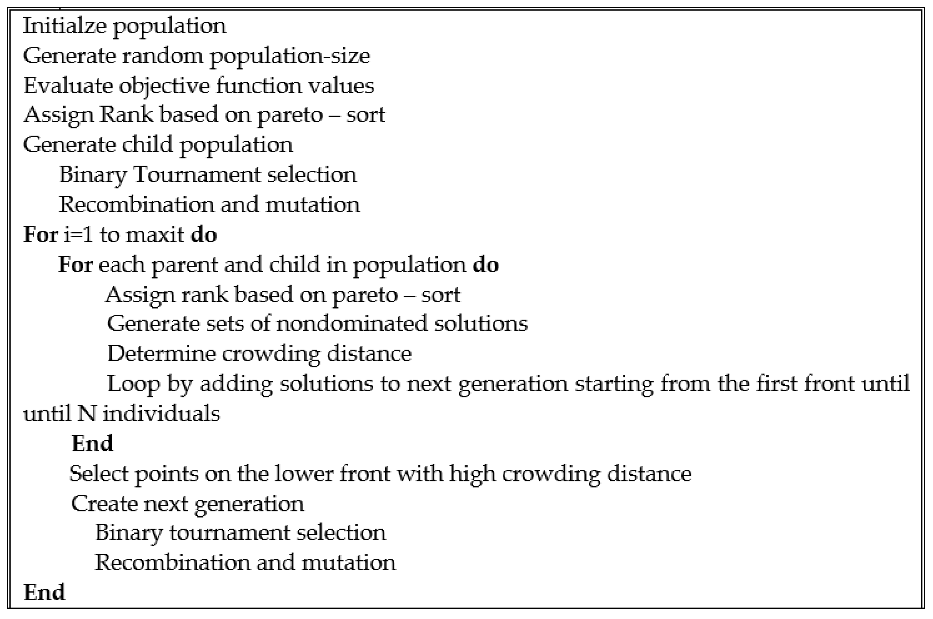
3.3. Psedou Code of Meta Heuristics Algorithm

In the designed SCN, there is a combination of different decisions, such as facility location, routing and optimal flow allocation under uncertainty. Therefore, the model can be called an Np-Hard problem [73]. Because it is very hard and impossible to solve these problems with exact methods, and as the size of the problem increases, its calculation time also increases [74]. For this reason, two non-dominated sorting genetic algorithms (NSGA II) and multi-objective particle swarm optimization (MOPSO) algorithms have been used in this research, and their pseudocodes are presented in Figure 3 and Figure 4.

4. Analysis of Results

In this part of the article, the issue is addressed according to

Table 2. The value of parameters.

Scenario	Parameter	Interval Limits
All Scenario	$Fix{I}_i,Fix{J}_j,Fix{L}_l,Fix{K}_k$	$~U\left[\mathrm{10,000},\mathrm{12,000}\right]$
	$Fix{V}_v$	$~U\left[300,400\right]$
	$Cap{V}_v$	$~U\left[100,120\right]$
	$Cap{L}_{lp},Cap{I}_{ir},Cap{K}_{kr},Cap{J}_{jp},{\mu }_l$	$~U\left[200,220\right]$
	$Di{s}_{n{n}^{\prime }}$	$~U\left[10,100\right]$
	$C{T}_l$	$~U\left[120,150\right]$
	${\mu }_l$	$~U\left[140,180\right]$
	${\theta }_l,p_s,r_p^c$	$0.5$
	$T_{n{n}^{\prime }}$	$~U\left[15,20\right]$
	$S_c,C_{lp}$	$~U\left[2,5\right]$
	$[A{S}_c,B{S}_c]$	$~U\left[20,50\right]$
	$\alpha$	$6$
	$H$	$3$
	${\omega }_{rp}$	$~U\left[1,2\right]$
	${\vartheta }_l$	$~U\left[3,4\right]$
	$B_l$	$~U\left[250,300\right]$
Scenario 1	$T{r}_{n{n}^{\prime }vs},T{r}_{ikvs},T{r}_{kjvs},T{r}_{jlvs},T{r}_{ljvs},T{r}_{lovs}$	$~U\left(\left[10,20\right],\left[20,30\right],\left[30,40\right],\left[40,50\right]\right)$
	$D_{cpts}$	$~U\left(\left[15,20\right],\left[20,25\right],\left[25,30\right],\left[30,35\right]\right)$
	$R_{cpts}$	$~U\left(\left[5,10\right],\left[10,15\right],\left[15,20\right],\left[20,25\right]\right)$
Scenario 2	$T{r}_{n{n}^{\prime }vs},T{r}_{ikvs},T{r}_{kjvs},T{r}_{jlvs},T{r}_{ljvs},T{r}_{lovs}$	$~U\left(\left[12,24\right],\left[24,36\right],\left[36,48\right],\left[48,60\right]\right)$
	$D_{cpts}$	$~U\left(\left[20,25\right],\left[25,30\right],\left[30,35\right],\left[35,40\right]\right)$
	$R_{cpts}$	$~U\left(\left[10,15\right],\left[15,20\right],\left[20,25\right],\left[25,30\right]\right)$

in order to satisfy the requirements of a small sample according to

Table 3. Small sample problem size.

$I-J-K-L-C-N-O-R-P-T-V-S$

$2-2-2-2-3-2-2-2-1-2-2-2$

and on the basis of random parameters. Because we do not have access to data taken from the actual world and because we are in the process of developing a mathematical model, we have been using random data that is based on the uniform distribution function.

The three-objective model is solved using the comprehensive multi-objective decision-making approach with the Baron solver in GAMS software once the issue has been designed and the problem range has been presented. Before attempting to solve the model, an exhaustive approach to making decisions that take into account several objectives is first described. When making decisions based on comprehensive criteria, it is necessary to do individual optimization in order to acquire the greatest possible value for each OBF. To put it another way, the program has to first determine the value of each OBF on its own without taking into account any of the other functions that will be utilized in the computations. The multi-objective decision-making process is represented as a complete one in Equation (88), which may be found below.

$$L_p=w_1\left(\frac{\left(f_1-f_1^{*}\right)}{\left(f_1^{*}\right)}\right)+w_2\left(\frac{\left(f_2-f_2^{*}\right)}{\left(f_2^{*}\right)}\right)+w_3\left(\frac{\left(f_3-f_3^{*}\right)}{\left(f_3^{*}\right)}\right)$$

(87)

In the above relation, $f_{i=1,2,3}$ the OBF of the i th problem, $f_{i=1,2,3}^{*}$ the best value of the OBF obtained from the individual optimization method and $w_{i=1,2,3}$ is the weight assigned to each OBF. In this research, linear softness, i.e., $p=1$ and random weights based on the Monte Carlo method, have been used.

Table 4. OBFV and CPU-time obtained by individual optimization method.

OBF	Value	CPU-Time
OBFV1	347,389.77	285.54
OBFV2	12,822.22	360.46
OBFV2	37.54	188.39

shows the optimal value of each OBF by individual optimization methods.

From solving the small-size numerical example, 8 efficient solutions in 30 consecutive repetitions of the Monte Carlo method are obtained, which are shown in

Table 5. The set of efficient solutions obtained from solving the small size problem.

Efficient Solutions	OBFV1	OBFV2	OBFV3
1	352,373	131,062	41
2	351,263	131,054	54
3	350,043	130,998	63
4	348,895	130,983	74
5	348,849	130,897	89
6	347,795	130,839	103
7	346,218	129,746	112
8	345,233	128,864	120

. Figure 5 also shows the Pareto front created between different target functions.

According to Table 5 and Figure 5, vehicles with higher speeds and higher costs should be used, and the route of product transfer between centers should be changed to reduce the maximum traffic time of vehicles. This has led to an increase in shipping costs. According to this model, with the reduction of greenhouse gas emissions, transmission costs have also increased due to changes in the design of the network structure.

To examine the output variables of the problem, one of the efficient solutions (work solution number one out of the eight work solutions obtained) is examined to obtain changes in the problem decision variables. Based on the results of Table 5, it can be seen that the efficient solutions have not reached their optimal value and have a relative difference from the best value of the OBF.

Table 6. Locating and routing the vehicle in the small size problem for the first efficient solution.

Centers	Location
Supplier	2 centers with number 2–3
Crude oil silo	1 center with number 2
Production center	1 center with number 2
Distribution/collection center	2 centers with number 1–2
Vehicle routing-scenarion1-period1	$L1\to N2\to N3\to L1\hspace{1em}L2\to N1\to L2$
Vehicle routing-scenarion1-period2	$L1\to N2\to N3\to L1\hspace{1em}L2\to N1\to L2$
Vehicle routing-scenarion2-period1	$L1\to N1\to N2\to L1\hspace{1em}L2\to N3\to L2$
Vehicle routing-scenarion2-period2	$L1\to N1\to N2\to L1\hspace{1em}L2\to N3\to L2$

shows the location and routing of the vehicle in the first efficient solution obtained.

The sensitivity of the issue that is being analyzed, as well as the influence of changes in some of the problem parameters on the values of the OBFs, will be examined in more detail in the following paragraphs. As a result, the total quantity of greenhouse gas emissions produced by the SCN has been analyzed, and the results show that these emissions are 30%, 20% and 10% lower than their base value, respectively. The changes that take place in the values of the problem’s goal functions as a result of shifts in the total quantity of greenhouse gas emissions is outlined in

Table 7. OBFVs in changing effect of parameter H.

Changes of $H$(%)	OBFV1	OBFV2	OBFV3
−30	349,666	130,672	41
−20	350,471	130,727	41
−10	350,993	130,783	41
0	352,373	131,062	41
10	352,817	131,204	41
20	353,614	131,467	41
30	353,836	131,543	41

, which may be found below.

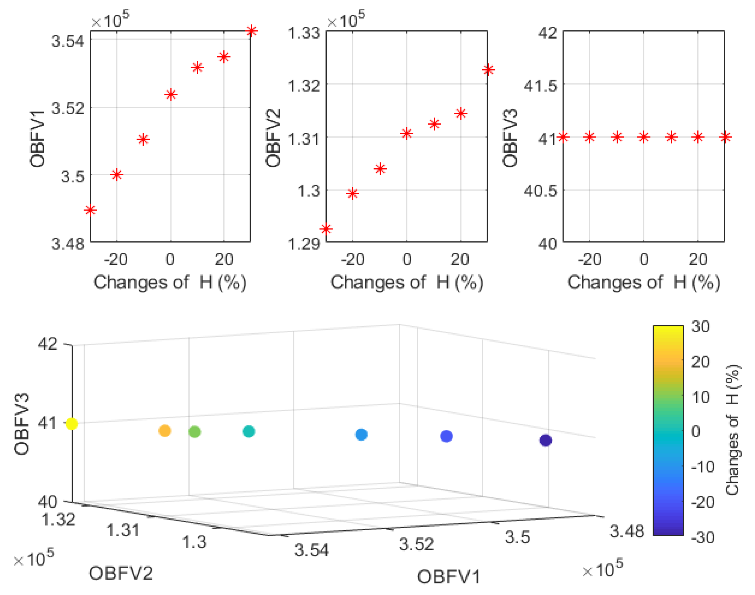
According to Table 7, it can be seen that the overall quantity of greenhouse gas emissions rose as a result of the direct influence that this parameter had on the second OBF of the issue. As a consequence of this, the total cost of the SCN design increased as well. despite the fact that the maximum amount of time spent in traffic did not change. The pattern of shifts in the values of the goal functions that occur in exchange for changes in the total quantity of greenhouse gas emissions is shown in Figure 6.

In the following, the the fine due to exceeding the time window is examined and its amount is 30%, 20% and 10% less and more than its base amount.

Table 8. OBFVs in changing effect of parameter α.

Changes of α (%)	OBFV1	OBFV2	OBFV3
−30	348,961	129,263	41
−20	350,009	129,938	41
−10	351,060	130,395	41
0	352,373	131,062	41
10	353,162	131,256	41
20	353,489	131,449	41
30	354,230	132,280	41

shows the change in the values of the OBFs of the problem in exchange for the change in the amount of the fine due to exceeding the time window.

According to Table 8, it can be seen that the overall cost of network design, as well as the amount of greenhouse gas emissions, has grown with the growing fines that have resulted from going over the allotted time frame. In addition, because this parameter does not have any impact on the third OBF of the issue, the maximum amount of time spent in traffic caused by vehicles does not change. Figure 7 illustrates the pattern of how the values of the goal functions shift over time in response to alterations in the total amount of the time window penalty.

In the end, an investigation is carried out to determine the pattern of shifts that occur in the values of the OBFs of the issue in exchange for shifts in the rate of uncertainty in a number of different problem situations. The goal of this investigation is to determine how these shifts come about. In this section, the changes that take place in the values of the issue’s goal functions in exchange for the changes that take place in the uncertainty rate are presented. The values range from 0.1 to 0.9. These results are derived from an examination of the issues in question that was carried out with an uncertainty rate of 0.5.

Table 9. OBFVs in changing effect of parameter α_s.

Changes of αs	OBFV1	OBFV2	OBFV3
0.1	347,647	128,829	38
0.3	350,470	130,183	39
0.5	352,373	131,062	41
0.7	353,742	133,330	43
0.9	356,462	134,240	44

displays, for a variety of uncertainty rates, the pattern of shifts that take place in the values of OBFs as they go through their lifetimes.

According to Table 9, it can be shown that the quantity of demand in the network grows with the rate of uncertainty. This, in turn, has a direct influence on the expenses of the whole network, the amount of greenhouse gas emissions and the maximum amount of time a vehicle spends in traffic. Figure 8 also demonstrates the effects of the uncertainty rate on the values of the goal functions and explains how those changes occurred.

Following the completion of the analysis of the sample problem in its small size, the NSGA II and MOPSO are used to complete the solution of the sample issue in its big size. As a result, before attempting to solve the issue, the parameters of the algorithms that have been stated are first specified and then an initial solution to the problem is presented.

The Taguchi technique requires that first the important components be recognized, then the levels of each element be decided, and finally the suitable test design for these control factors must be defined. The Taguchi method was developed by Kaoru Taguchi.

After the test design has been decided upon, the tests are carried out and then examined to see which combination of factors produces the best results. According to

Table 10. Proposed parameter levels for tuning of NSGA II and MOPSO.

Algorithm	Parameter	Level 1	Level 2	Level 3	Best Value
NSGA II	Max it	100	150	200	200
	Npop	50	100	200	200
	Pc	0.75	0.80	0.85	0.80
	Pm	0.03	0.035	0.04	0.03
MOPSO	Max it	100	150	200	200
	NParticle	50	100	200	200
	C1	1	1.5	2	1
	C2	1	1.5	2	2

, there have been three degrees of consideration given to each aspect during the course of this study. The design of the experiment and the manner in which it is to be carried out for each algorithm are both defined by the number of factors and the number of levels each factor has. In light of the fact that the proposed model incorporates three different goal functions, it is necessary to begin by deriving the value of each experiment from Equation (89). In this regard, in the case of subtraction of the indicators used in the comparison of meta-heuristic algorithms, including (the average of the first to third OBF, number of efficient solutions, maximum expansion index, metric distance index and computational time), has been used. Specifically, the average of the first to third OBF. In order to conduct an analysis of the design of the Taguchi experiment, the first step is to determine the value of each experiment. Subsequently, the scaled value of each experiment (RPD) is determined using Equation (89).

$$S_i=\left|\frac{MeanZ1+MeanZ2+MeanZ3+NPF+MSI+SM+CPU\_time}{7}\right|$$

(88)

$$RPD=\frac{S_i-S_i^{*}}{S_i^{*}}$$

(89)

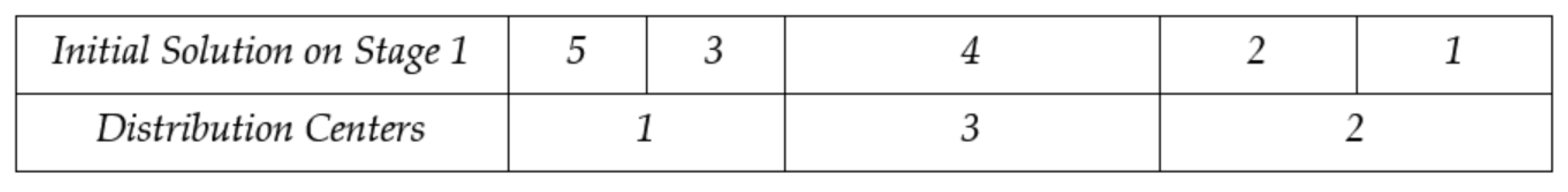
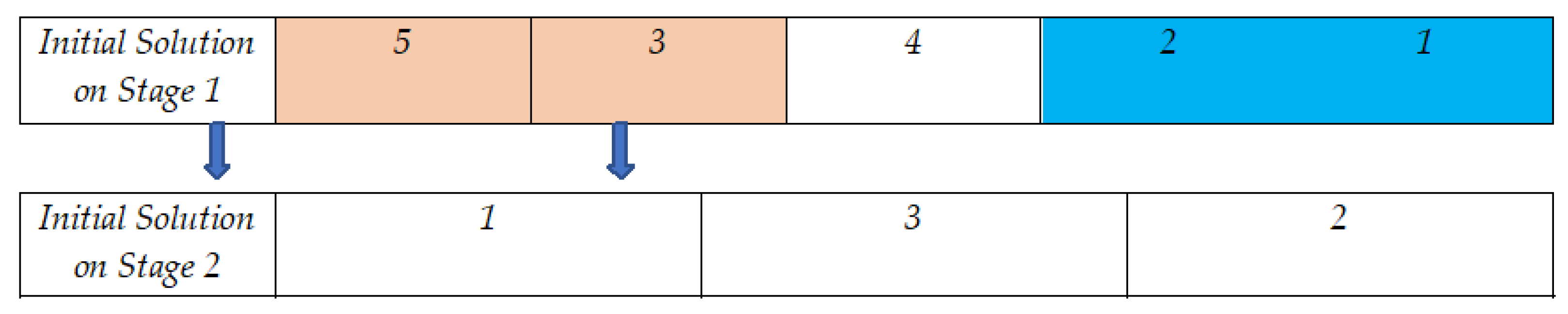
Based on the results of the Taguchi method in the parameterization of meta-heuristic algorithms, it is observed that the maximum number of iterations and also the number population in the two algorithms is equal to 200. After parameterizing the meta-heuristic algorithms, a primary chromosome is presented to solve the problem. Therefore, in this section, two different chromosomes are considered. The first part of the chromosome is related to the routing of the vehicle between the distribution centers and the customers, and the second part is related to the optimal location and the allocation of goods between other levels of the SC. Therefore, in the first part, assuming five customers and three distribution centers, the primary chromosome is presented according to Figure 9. In this chromosome, in the first level of the SCN, the substitution of natural numbers is first produced for the total number of customers.

The next step in the design of the chromosome is to decide which clients will be assigned to which intermediary warehouses. Therefore, the entire number of clients is arbitrarily distributed among the total number of distribution centers, and the path that the vehicle takes is determined by the numbers generated in the first level of the chromosome’s initial solution. Figure 8 demonstrates how customers are assigned to distribution locations, and Figure 9 illustrates how chromosomes are used to determine truck routing.

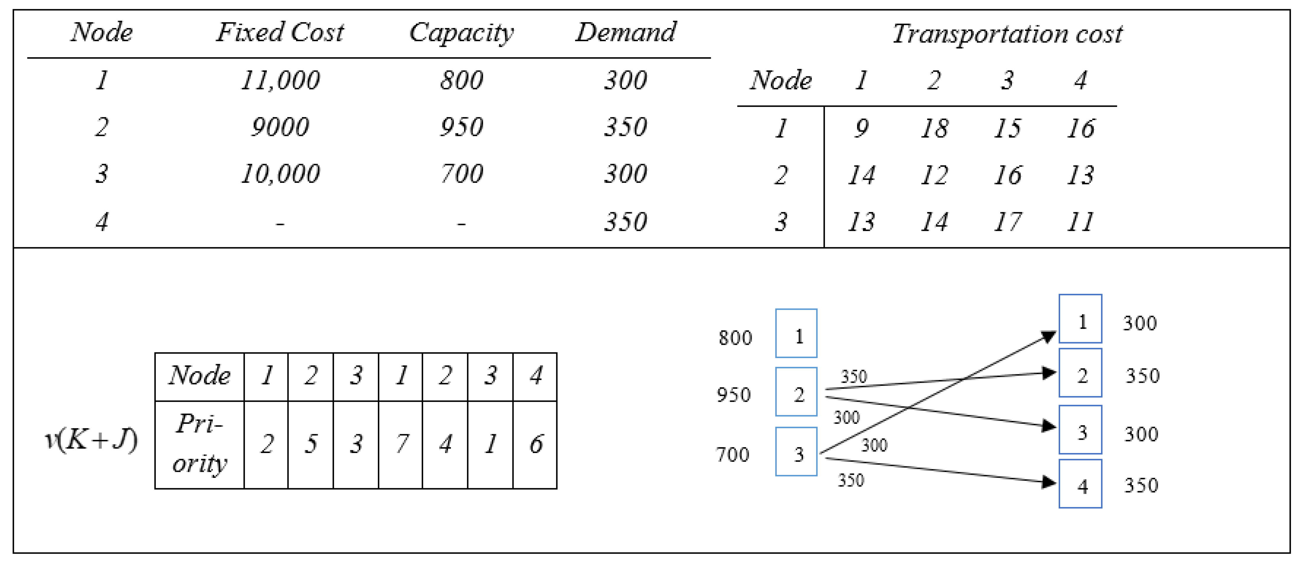
According to Figure 10, it is observed that customers 5 and 3 are allocated to distribution center 1, customer 4 is allocated to distribution center 3, and customers 2 and 1 are allocated to distribution center 2. Moreover, vehicle routing from distribution center 1 is $L1\to N5\to N3\to L1$, vehicle routing from distribution center 2 is $L3\to N4\to L3$. The second part of the chromosome discusses the location of the facility as well as the optimal allocation of flow between the selected facility. Hence another chromosome will be generated and decoded for each level of the SCN as follows. This encryption is based on a permutation of natural numbers to the number of nodes in each level of the two levels of the SCN. Figure 11 shows the priority-based encoding for one of the network levels with 3 major distribution centers and 4 fixed demand centers.

Encoding (6-1-4-7-3-5-2) that illustrates the priorities (7-4-1-6) for fixed demand centers and how (2-5-3) is connected to the distributor center is shown in Figure 9. In order to successfully decode anything, you will need to complete the following two steps:

Step 1—To begin, the donor with the highest number (priority) from the selected major distribution centers (priority 5 for the second major distribution center), and if this donor can meet all of the demands of the customer centers, the priority of the other donation centers will be reduced to zero. Step 2—If this donor cannot meet all of the demands of the customer centers, the donor with the next highest number (priority) from the major distribution centers will. Figure 11 presents an example in which the capacity of the main distribution center is shown to be two times 950; however, the total demand from the stationary client centers is shown to be 1300. In this instance, the distribution hub with the second greatest priority on the list is chosen to be the subsequent main one (priority 3 related to the third major distribution center). Now, the combined total capacity of the two main distribution centers, which is 1650, is more than the combined total demand of the client centers (amount 1300). In such a scenario, the priority of just the very first big distribution center will be lowered all the way to zero.

Step 2: The ideal allocation is established between the main distribution centers that have been chosen and the demand centers once it has been determined how many prospective major distribution centers there are and where they are located. In this stage, the highest priority is selected (priority 7, which is related to the first demand center), and the lowest transportation cost related to this customer is identified with the major distribution center that was selected from the first stage (the third donor center at a cost of 15), along with the distribution center’s minimum capacity. The ideal allocation amount is computed, and it is decided to go to the chosen major and the given consumer. After increasing the available capacity or satisfying any remaining unmet demand, the priority will be lowered to zero. The second step is performed several times until the values of all the priorities have been brought down to zero.

According to the findings for large sample (see Table 10) presented in

Table 11. Large-size sample problem.

Sample Problem	$I$	$J$	$K$	$O$	$C$	$R$	$S$	$L$	$P$	$V$	$T$
1	10	10	10	10	12	2	2	10	6	6	4
2	10	10	10	10	14	2	2	12	6	6	4
3	10	10	10	10	16	2	2	14	6	6	4
4	12	12	12	12	18	2	3	16	7	8	5
5	12	12	12	12	20	3	3	18	7	8	5
6	12	12	12	12	22	3	3	20	7	8	5
7	15	15	15	15	24	3	4	22	8	9	6
8	15	15	15	15	26	3	4	24	8	9	6
9	15	15	15	15	28	4	4	26	9	10	6
10	20	20	20	20	30	4	4	28	10	12	7
11	20	20	20	20	32	4	4	30	12	14	7
12	20	20	20	20	34	4	5	35	14	15	7
13	30	30	30	30	36	4	5	40	16	18	8
14	30	30	30	30	38	5	5	45	18	20	8
15	30	30	30	30	40	5	5	50	20	20	8

,

Table 12. The results of solving the large-size problem by NSGA II.

Sample Problem	OBFV1	OBFV2	OBFV3	NPF	MSI	SM	CPU-Time
1	5,171,405.41	2,185,833.07	111.22	78	13,812.22	0.47	49.50
2	5,398,994.99	2,762,386.33	154.71	82	15,289.78	0.35	54.96
3	6,019,488.06	3,177,521.50	172.35	78	13,967.83	0.49	72.67
4	6,423,286.41	4,097,302.32	181.45	86	25,449.48	0.70	127.99
5	6,538,955.89	4,479,863.43	241.63	99	21,730.77	0.53	211.19
6	6,785,707.08	5,184,306.28	281.41	83	25,579.07	0.35	293.14
7	7,158,871.09	5,171,757.20	307.80	90	11,585.14	0.45	417.93
8	7,510,548.53	5,866,537.72	332.89	84	19,542.07	0.58	531.23
9	8,203,753.18	6,163,001.94	357.24	87	13,608.73	0.41	651.28
10	8,752,921.66	7,404,421.13	382.46	82	24,953.18	0.50	800.82
11	9,632,491.97	7,679,581.39	418.87	89	15,643.39	0.45	946.15
12	9,964,265.20	7,753,593.48	430.39	93	20,804.43	0.33	1090.87
13	10,331,524.82	8,802,996.24	459.11	100	16,704.49	0.48	1288.36
14	10,898,039.49	9,128,745.36	481.50	88	17,739.98	0.32	1484.07
15	11,591,974.13	10,023,438.99	498.64	100	12,786.59	0.38	1741.28
Mean	8,025,481.86	5,992,085.76	320.78	87.93	17,946.48	0.45	650.76

and

Table 13. The results of solving the large-size problem by MOPSO.

Sample Problem	OBFV1	OBFV2	OBFV3	NPF	MSI	SM	CPU-Time
1	4,848,705.20	2,246,354.07	112.48	87	13,893.62	0.11	36.12
2	5,105,061.04	2,774,160.60	156.37	87	15,360.07	0.84	40.26
3	6,154,917.34	3,229,399.79	173.93	73	14,187.67	0.06	67.47
4	6,348,347.09	4,077,913.22	184.79	95	24,971.92	0.00	110.46
5	6,186,380.36	4,385,821.23	240.44	93	21,266.31	0.93	192.41
6	6,495,843.04	5,102,888.86	277.56	96	24,068.86	0.64	259.46
7	7,013,609.31	5,301,333.88	315.55	76	11,096.09	0.84	378.08
8	7,469,621.09	6,087,316.25	346.42	90	19,320.87	0.20	484.95
9	8,055,298.63	6,615,262.62	371.42	97	13,565.07	0.99	599.87
10	8,759,362.34	7,444,580.76	396.65	96	23,552.83	0.81	702.82
11	9,823,948.57	8,024,997.44	416.51	78	15,517.71	0.81	828.01
12	9,709,571.06	8,182,310.00	435.42	96	21,184.23	0.80	953.14
13	9,828,373.25	8,925,208.72	457.80	99	15,826.70	0.47	1093.42
14	10,171,326.13	9,752,619.14	480.31	83	17,106.66	0.58	1298.98
15	11,678,009.44	9,990,665.72	502.79	95	12,995.98	0.86	1565.99
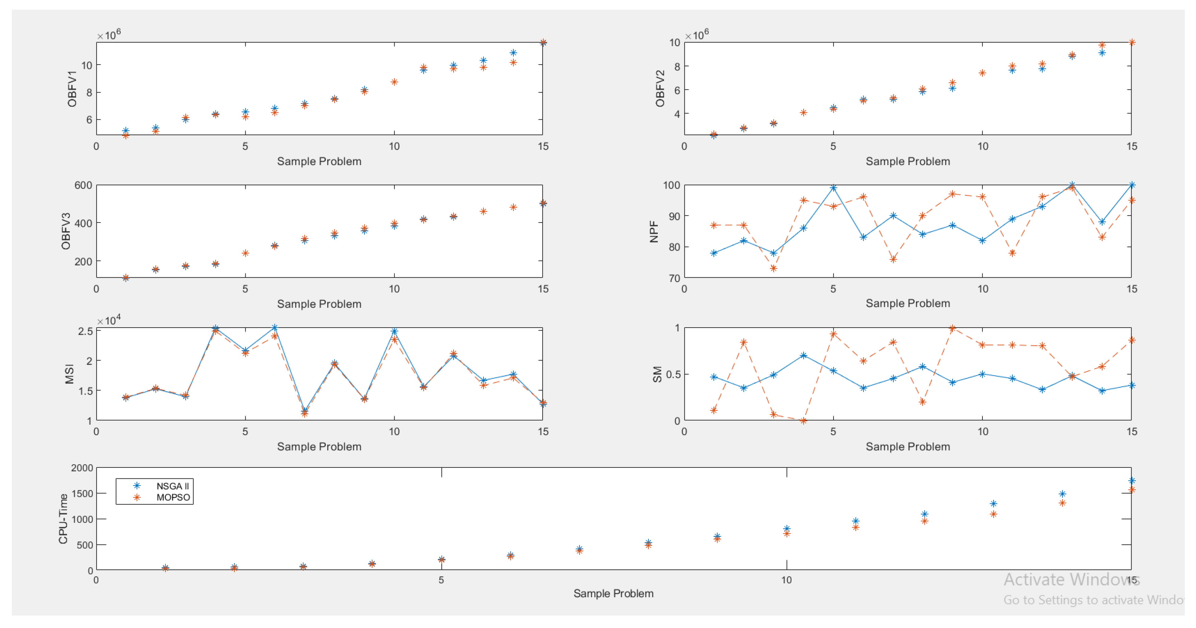
Mean	7,843,224.93	6,142,722.15	324.56	89.40	17,594.31	0.60	574.10

, it has been observed that the value of the first OBF all the way up to the third OBF has increased as the size of the problem has grown. This is because the number of customers has grown and estimates of their demand have been made. Moreover, as the size of the issue has grown, the amount of time required to solve the problem has risen exponentially, which is an indication of the rigidity of the model that has been provided. It has also been noticed that in terms of algorithm performance, NSGA II has a better average of the second and third OBFs, maximum spread index (MSI) and spacing metric (SM) index, when compared to MOPSO. These indices refer to maximum spread index and spacing metric, respectively. Figure 12 presents a comparison of the results that were achieved when large-scale numerical cases were solved using two different techniques.

According to the diagram in Figure 12, it can be seen that as the size of the problem increases, the computational time increases exponentially, which is proof that the problem is NP-Hard. Moreover, with increasing the computational time, the mean of the OBFs has increased and the most significant increase has been in the changes of periods.

Since each of the algorithms has been successful in obtaining a specific index and the weighted average of the results has been close to each other. Therefore, a t-test at a 95% confidence level was used to evaluate the significant difference between the mean results.

Table 14. Results of t-test.

Index	Difference of Mean	95% CI for Mean Different	T-Value	p-Value
OBFV1	182,257	(45,034 319,480)	2.85	0.013
OBFV2	150,636	(30,215 271,057)	2.68	0.018
OBFV3	3.78	(0.42 7.15)	2.41	0.030
NPF	1.47	(−3.43 6.36)	0.64	0.531
MSI	352	(36 668)	2.39	0.031
SM	0.143	(−0.084 0.371)	1.35	0.198
CPU-Time	76.7	(38.7 114.7)	4.33	0.001

summarizes these results.

According to the results of Table 14 and the value of p-value, it is observed that there is a significant difference between the means of the OBFs, the maximum expansion and computational time between the two algorithms, and therefore, it is not possible to prefer the algorithms to each other. Therefore, using the TOPSIS method, a more efficient algorithm has been selected (see

Table 15. The results of TOPSIS method.

Algorithm	OBFV1	OBFV2	OBFV3	NPF	MSI	SM	CPU-Time
NSGA II	8,025,481.86	5,992,085.76	320.78	87.93	17,946.48	0.45	650.76
MOPSO	7,843,224.93	6,142,722.15	324.56	89.40	17,594.31	0.60	574.10
weight	0.2	0.2	0.2	0.1	0.1	0.1	0.1

).

After the above analysis, the NSGA II with a gain weight of 0.6832 and the MOPSO with a gain weight of 0.3168, respectively, are recognized as the most efficient algorithm for solving the problem.

5. Conclusions

The ever-increasing growth of urbanization, as well as industries, particularly support sectors, has resulted in the movement of both people and things, which has led to an issue whose complexity is continually growing. The growth of cities has led to an increase in the demand placed on the transportation sector. This, in turn, has led to an increase in the number of challenges faced by cities and large industries, including an increase in the amount of time wasted traveling, an increase in the amount of fuel used and an increase in the value of vehicles. It is necessary to have a transportation system that is both well-equipped and efficient in order to alleviate traffic difficulties and the subsequent economic, social and environmental issues that they cause in big cities, manufacturing enterprises and service-oriented businesses. The transportation industry is both a substantial and crucial component of every nation’s economy, as well as one of the most important factors in determining the final price of completed goods. Because of the significance of product transfer, this investigation was undertaken to simulate and find a solution to a challenge posed by a CLSC operating in an unpredictable environment. The researchers took into account the queuing system, as well as simultaneous delivery and harvesting. In light of this, the study in question takes into account a seven-tiered SCN, which includes raw material suppliers, storage facilities (silos), production centers, distribution centers, end customers, collecting centers and destruction centers. In this scenario, the suppliers of raw materials provided to the warehouses the raw materials that are required for the production of the final goods (silos). At the next level of the SC network (SCN), production centers take the raw materials that they receive from silos and collection centers and use those commodities to make finished goods, which are then distributed to customers through distribution centers. After the items have been sorted into their appropriate categories, distribution facilities next send them on to clients via the appropriate method of transportation.

When it comes to the return chain, consumers end up throwing away a certain proportion of the things they purchase after using them. Following the collection and inspection of the products as well as their transformation into raw materials or scrap, the collection centers allocate a certain percentage of the products for reproduction to production centers and a certain percentage of the products for destruction centers. The primary objective of this network is to reduce overall SCN costs as much as possible. These costs include location, allocation and routing expenses. In order to address the issue, a simplified model was developed, and then that model was solved with the use of an all-encompassing multi-objective decision-making process. The end result was the production of eight effective solutions. After looking at the output variables of the problem, it was discovered that the value of the first and second OBFs has increased as the amount of the fine for exceeding the time window and the amount of greenhouse gas emissions have increased. This was one of the observations that were made after the examination of the output variables of the problem. Following that, NSGA II and MOPSO were used since the GAMS program proved to be ineffective. As a result, 15 different sample issues were devised and tested on bigger scales.

When the magnitude of the issue expanded, the amount of time needed to solve it also climbed exponentially. Therefore, the issue at hand is one that falls within the NP-Hard category of problems. The conclusion that could be drawn from the findings of the study that compared the two algorithms was that the NSGA II is more effective at finding solutions to problems. The findings that were acquired from the presentation of the mathematical model in this article may be of assistance to managers in cutting expenses and lowering the amount of dispersion that is brought about by the SC of manufacturing units. Within this model, a variety of efficient solutions have been presented, and as a result, managers may be able to improve their decision-making abilities, both in terms of the choices they make at the strategic and tactical levels. Additionally, the fact that the mathematical model has an uncertainty rate is of great assistance to the managers of production units in predicting the costs that are likely to be incurred on the SC under the most pessimistic and optimistic scenarios. It is proposed as a future study that the OBF of dependability in the distribution of goods to consumers and the problem of resilience in the CLSC network be both studied. Additionally, it is advised that the issue of resilience in the CLSC network be considered. Additionally, the optimization of one’s capacity to fulfill one’s societal duties has to be included in the mathematical model as well. In order to speed up the process of issue-solving, it has also been recommended that hybrid meta-heuristic algorithms be developed.

References

1. Asim, Z.; Jalil, S.A.; Javaid, S. An uncertain model for integrated production-transportation closed-loop supply chain network with cost reliability. Sustain. Prod. Consum. 2018, 17, 298–310. [Google Scholar] [CrossRef]
2. Guide, V.D.R., Jr.; Van Wassenhove, L.N. OR FORUM—The evolution of closed-loop supply chain research. Oper. Res. 2009, 57, 10–18. [Google Scholar] [CrossRef]
3. Govindan, K.; Mina, H.; Esmaeili, A.; Gholami-Zanjani, S.M. An Integrated Hybrid Approach for Circular supplier selection and Closed loop Supply Chain Network Design under Uncertainty. J. Clean. Prod. 2019, 242, 118317. [Google Scholar] [CrossRef]
4. Govindan, K.; Soleimani, H.; Kannan, D. Reverse logistics and closed-loop supply chain: A comprehensive review to explore the future. Eur. J. Oper. Res. 2015, 240, 603–626. [Google Scholar] [CrossRef] [Green Version]
5. Rogers, D.S.; Tibben-Lembke, R.S. Going Backwards: Reverse Logistics Trends and Practices; Reverse Logistics Executive Council: Pittsburgh, PA, USA, 1999. [Google Scholar]
6. Liao, H.; Deng, Q.; Shen, N. Optimal remanufacture-up-to strategy with uncertainties in acquisition quality, quantity, and market demand. J. Clean. Prod. 2018, 206, 987–1003. [Google Scholar] [CrossRef]
7. Liao, H.; Deng, Q.; Wang, Y.; Guo, S.; Ren, Q. An environmental benefits and costs assessment model for remanufacturing process under quality uncertainty. J. Clean. Prod. 2018, 178, 45–58. [Google Scholar] [CrossRef]
8. Pokharel, S.; Mutha, A. Perspectives in reverse logistics: A review. Resour. Conserv. Recycl. 2009, 53, 175–182. [Google Scholar] [CrossRef]
9. Zhalechian, M.; Tavakkoli-Moghaddam, R.; Zahiri, B.; Mohammadi, M. Sustainable design of a closed-loop location-routing-inventory supply chain network under mixed uncertainty. Transp. Res. Part E Logist. Transp. Rev. 2016, 89, 182–214. [Google Scholar] [CrossRef]
10. Hatefi, S.; Jolai, F.; Torabi, S.A.; Tavakkoli-Moghaddam, R. A credibility-constrained programming for reliable forward–reverse logistics network design under uncertainty and facility disruptions. Int. J. Comput. Integr. Manuf. 2014, 28, 664–678. [Google Scholar] [CrossRef]
11. Li, J.; Wang, S.; Cheng, E. Competition and cooperation in a single-retailer two-supplier supply chain with supply disruption. Int. J. Prod. Econ. 2010, 124, 137–150. [Google Scholar] [CrossRef]
12. Ahi, P.; Jaber, M.Y.; Searcy, C. A comprehensive multidimensional framework for assessing the performance of sustainable supply chains. Appl. Math. Model. 2016, 40, 10153–10166. [Google Scholar] [CrossRef]
13. Simchi-Levi, D.; Kaminsky, P.; Simchi-Levi, E. Managing the Supply Chain: The Definitive Guide for the Business Professional; McGraw-Hill: New York, NY, USA, 2004. [Google Scholar]
14. Guo, W.; Atasoy, B.; Negenborn, R.R. Global synchromodal shipment matching problem with dynamic and stochastic travel times: A reinforcement learning approach. Ann. Oper. Res. 2022. [Google Scholar] [CrossRef]
15. Keyvanshokooh, E.; Fattahi, M.; Seyed-Hosseini, S.; Tavakkoli-Moghaddam, R. A dynamic pricing approach for returned products in integrated forward/reverse logistics network design. Appl. Math. Model. 2013, 37, 10182–10202. [Google Scholar] [CrossRef]
16. Zokaee, S.; Jabbarzadeh, A.; Fahimnia, B.; Sadjadi, S.J. Robust supply chain network design: An optimization model with real world application. Ann. Oper. Res. 2014, 257, 15–44. [Google Scholar] [CrossRef]
17. Vahdani, B.; Mohammadi, M. A bi-objective interval-stochastic robust optimization model for designing closed loop supply chain network with multi-priority queuing system. Int. J. Prod. Econ. 2015, 170, 67–87. [Google Scholar] [CrossRef]
18. Lalmazloumian, M.; Wong, K.Y.; Govindan, K.; Kannan, D. A robust optimization model for agile and build-to-order supply chain planning under uncertainties. Ann. Oper. Res. 2013, 240, 435–470. [Google Scholar] [CrossRef]
19. Hernandez, I.; Ramirez-Marquez, J.E.; Rainwater, C.; Pohl, E.; Medal, H. Robust facility location: Hedging against failures. Reliab. Eng. Syst. Saf. 2014, 123, 73–80. [Google Scholar] [CrossRef]
20. Ghomi-Avili, M.; Naeini, S.G.J.; Tavakkoli-Moghaddam, R.; Jabbarzadeh, A. A fuzzy pricing model for a green competitive closed-loop supply chain network design in the presence of disruptions. J. Clean. Prod. 2018, 188, 425–442. [Google Scholar] [CrossRef]
21. Zhang, Z.; Liu, S.; Niu, B. Coordination mechanism of dual-channel closed-loop supply chains considering product quality and return. J. Clean. Prod. 2019, 248, 119273. [Google Scholar] [CrossRef]
22. Pazhani, S.; Mendoza, A.; Nambirajan, R.; Narendran, T.; Ganesh, K.; Olivares-Benitez, E. Multi-period multi-product closed loop supply chain network design: A relaxation approach. Comput. Ind. Eng. 2021, 155, 107191. [Google Scholar] [CrossRef]
23. Mehrjerdi, Y.Z.; Shafiee, M. A resilient and sustainable closed-loop supply chain using multiple sourcing and information sharing strategies. J. Clean. Prod. 2020, 289, 125141. [Google Scholar] [CrossRef]
24. Fu, L.; Tang, J.; Meng, F. A disease transmission inspired closed-loop supply chain dynamic model for product collection. Transp. Res. Part E Logist. Transp. Rev. 2021, 152, 102363. [Google Scholar] [CrossRef]
25. Khorshidvand, B.; Soleimani, H.; Sibdari, S.; Esfahani, M.M.S. Developing a two-stage model for a sustainable closed-loop supply chain with pricing and advertising decisions. J. Clean. Prod. 2021, 309, 127165. [Google Scholar] [CrossRef]
26. Zheng, B.; Chu, J.; Jin, L. Recycling channel selection and coordination in dual sales channel closed-loop supply chains. Appl. Math. Model. 2021, 95, 484–502. [Google Scholar] [CrossRef]
27. Hornstra, R.P.; Silva, A.; Roodbergen, K.J.; Coelho, L.C. The vehicle routing problem with simultaneous pick-up and delivery and handling costs. Comput. Oper. Res. 2020, 115, 104858. [Google Scholar] [CrossRef]
28. Olgun, B.; Koç, Ç.; Altıparmak, F. A hyper heuristic for the green vehicle routing problem with simultaneous pick-up and delivery. Comput. Ind. Eng. 2021, 153, 107010. [Google Scholar] [CrossRef]
29. Agra, A.; Christiansen, M.; Wolsey, L. Improved models for a single vehicle continuous-time inventory routing problem with pick-ups and deliveries. Eur. J. Oper. Res. 2022, 297, 164–179. [Google Scholar] [CrossRef]
30. Fan, H.; Zhang, Y.; Tian, P.; Lv, Y.; Fan, H. Time-dependent multi-depot green vehicle routing problem with time windows considering temporal-spatial distance. Comput. Oper. Res. 2021, 129, 105211. [Google Scholar] [CrossRef]
31. Sadati, M.E.H.; Çatay, B. A hybrid variable neighborhood search approach for the multi-depot green vehicle routing problem. Transp. Res. Part E Logist. Transp. Rev. 2021, 149, 102293. [Google Scholar] [CrossRef]
32. Wang, Y.; Li, Q.; Guan, X.; Xu, M.; Liu, Y.; Wang, H. Two-echelon collaborative multi-depot multi-period vehicle routing problem. Expert Syst. Appl. 2020, 167, 114201. [Google Scholar] [CrossRef]
33. Zhen, L.; Ma, C.; Wang, K.; Xiao, L.; Zhang, W. Multi-depot multi-trip vehicle routing problem with time windows and release dates. Transp. Res. Part E Logist. Transp. Rev. 2020, 135, 101866. [Google Scholar] [CrossRef]
34. Soeanu, A.; Ray, S.; Berger, J.; Boukhtouta, A.; Debbabi, M. Multi-depot vehicle routing problem with risk mitigation: Model and solution algorithm. Expert Syst. Appl. 2019, 145, 113099. [Google Scholar] [CrossRef]
35. Bezerra, S.N.; Souza, M.J.F.; de Souza, S.R.; Coelho, V.N. A VNS-Based Algorithm with Adaptive Local Search for Solving the Multi-Depot Vehicle Routing Problem. In International Conference on Variable Neighborhood Search; Springer: Berlin/Heidelberg, Germany, 2019; pp. 167–181. [Google Scholar] [CrossRef]
36. Li, Y.; Soleimani, H.; Zohal, M. An improved ant colony optimization algorithm for the multi-depot green vehicle routing problem with multiple objectives. J. Clean. Prod. 2019, 227, 1161–1172. [Google Scholar] [CrossRef]
37. Nguyen, P.K.; Crainic, T.G.; Toulouse, M. A tabu search for Time-dependent Multi-zone Multi-trip Vehicle Routing Problem with Time Windows. Eur. J. Oper. Res. 2013, 231, 43–56. [Google Scholar] [CrossRef]
38. Wang, C.; Guo, C.; Zuo, X. Solving multi-depot electric vehicle scheduling problem by column generation and genetic algorithm. Appl. Soft Comput. 2021, 112, 107774. [Google Scholar] [CrossRef]
39. Sherif, S.U.; Asokan, P.; Sasikumar, P.; Mathiyazhagan, K.; Jerald, J. Integrated optimization of transportation, inventory and vehicle routing with simultaneous pick-up and delivery in two-echelon green supply chain network. J. Clean. Prod. 2021, 287, 125434. [Google Scholar] [CrossRef]
40. Silva, A.; Coelho, L.C.; Darvish, M.; Renaud, J. Integrating storage location and order picking problems in warehouse planning. Transp. Res. Part E Logist. Transp. Rev. 2020, 140, 102003. [Google Scholar] [CrossRef]
41. Araghi, M.E.T.; Tavakkoli-Moghaddam, R.; Jolai, F.; Molana, S.M.H. A green multi-facilities open location-routing problem with planar facility locations and uncertain customer. J. Clean. Prod. 2020, 282, 124343. [Google Scholar] [CrossRef]
42. Bruni, M.E.; Toan, D.Q.; Nam, L.H. The multi-vehicle profitable pick up and delivery routing problem with uncertain travel times. Transp. Res. Procedia 2021, 52, 509–516. [Google Scholar] [CrossRef]
43. Sitek, P.; Wikarek, J.; Rutczyńska-Wdowiak, K.; Bocewicz, G.; Banaszak, Z. Optimization of capacitated vehicle routing problem with alternative delivery, pick-up and time windows: A modified hybrid approach. Neurocomputing 2020, 423, 670–678. [Google Scholar] [CrossRef]
44. Martins, L.D.C.; Bayliss, C.; Juan, A.A.; Panadero, J.; Marmol, M. A Savings-Based Heuristic for Solving the Omnichannel Vehicle Routing Problem with Pick-up and Delivery. Transp. Res. Procedia 2020, 47, 83–90. [Google Scholar] [CrossRef]
45. Zachariadis, E.E.; Tarantilis, C.D.; Kiranoudis, C.T. The load-dependent vehicle routing problem and its pick-up and delivery extension. Transp. Res. Part B Methodol. 2015, 71, 158–181. [Google Scholar] [CrossRef]
46. Bektaş, T.; Gouveia, L.; Santos, D. Compact formulations for multi-depot routing problems: Theoretical and computational comparisons. Comput. Oper. Res. 2020, 124, 105084. [Google Scholar] [CrossRef]
47. Bertazzi, L.; Coelho, L.C.; De Maio, A.; Laganà, D. A matheuristic algorithm for the multi-depot inventory routing problem. Transp. Res. Part E Logist. Transp. Rev. 2019, 122, 524–544. [Google Scholar] [CrossRef]
48. Manupati, V.K.; Schoenherr, T.; Wagner, S.M.; Soni, B.; Panigrahi, S.; Ramkumar, M. Convalescent plasma bank facility location-allocation problem for COVID-19. Transp. Res. Part E Logist. Transp. Rev. 2021, 156, 102517. [Google Scholar] [CrossRef]
49. Khalili-Damghani, K.; Tavana, M.; Ghasemi, P. A stochastic bi-objective simulation–optimization model for cascade disaster location-allocation-distribution problems. Ann. Oper. Res. 2021, 309, 103–141. [Google Scholar] [CrossRef]
50. Aghaei Fishani, B.; Mahmoodirad, A.; Niroomand, S.; Fallah, M. Multi-objective location-allocation-routing problem of perishable multi-product supply chain with direct shipment and open routing possibilities under sustainability. Concurr. Comput. Pract. Exp. 2022, 34, e6860. [Google Scholar] [CrossRef]
51. Szmelter-Jarosz, A.; Ghahremani-Nahr, J.; Nozari, H. A Neutrosophic Fuzzy Optimisation Model for Optimal Sustainable Closed-Loop Supply Chain Network during COVID-19. J. Risk Financial Manag. 2021, 14, 519. [Google Scholar] [CrossRef]
52. Ahmed, S.; King, A.J.; Parija, G. A Multi-Stage Stochastic Integer Programming Approach for Capacity Expansion under Uncertainty. J. Glob. Optim. 2003, 26, 3–24. [Google Scholar] [CrossRef]
53. Song, M.; Gao, C.; Shahidehpour, M.; Li, Z.; Yang, J.; Yan, H. Impact of Uncertain Parameters on TCL Power Capacity Calculation via HDMR for Generating Power Pulses. IEEE Trans. Smart Grid 2018, 10, 3112–3124. [Google Scholar] [CrossRef]
54. Zhang, W.-G.; Liu, Y.-J.; Xu, W.-J. A new fuzzy programming approach for multi-period portfolio optimization with return demand and risk control. Fuzzy Sets Syst. 2014, 246, 107–126. [Google Scholar] [CrossRef]
55. Mousavi, S.M.; Niaki, S.T.A. Capacitated location allocation problem with stochastic location and fuzzy demand: A hybrid algorithm. Appl. Math. Model. 2013, 37, 5109–5119. [Google Scholar] [CrossRef]
56. Bertsimas, D.; Thiele, A. A robust optimization approach to supply chain management. In International Conference on Integer Programming and Combinatorial Optimization; Springer: Berlin/Heidelberg, Germany, 2004; pp. 86–100. [Google Scholar]
57. Pishvaee, M.S.; Rabbani, M.; Torabi, S.A. A robust optimization approach to closed-loop supply chain network design under uncertainty. Appl. Math. Model. 2011, 35, 637–649. [Google Scholar] [CrossRef]
58. Duque, D.; Mehrotra, S.; Morton, D.P. Distributionally Robust Two-Stage Stochastic Programming. SIAM J. Optim. 2022, 32, 1499–1522. [Google Scholar] [CrossRef]
59. Yin, X.; Büyüktahtakın, I.E. A multi-stage stochastic programming approach to epidemic resource allocation with equity considerations. Health Care Manag. Sci. 2021, 24, 597–622. [Google Scholar] [CrossRef]
60. Nozari, H.; Ghahremani-Nahr, J.; Szmelter-Jarosz, A. A multi-stage stochastic inventory management model for transport companies including several different transport modes. Int. J. Manag. Sci. Eng. Manag. 2022. [Google Scholar] [CrossRef]
61. Li, C.; Cai, Y.; Qian, J. A multi-stage fuzzy stochastic programming method for water resources management with the consideration of ecological water demand. Ecol. Indic. 2018, 95, 930–938. [Google Scholar] [CrossRef]
62. Nayeri, S.; Paydar, M.M.; Asadi-Gangraj, E.; Emami, S. Multi-objective fuzzy robust optimization approach to sustainable closed-loop supply chain network design. Comput. Ind. Eng. 2020, 148, 106716. [Google Scholar] [CrossRef]
63. Fathollahi-Fard, A.M.; Dulebenets, M.A.; Hajiaghaei–Keshteli, M.; Tavakkoli-Moghaddam, R.; Safaeian, M.; Mirzahosseinian, H. Two hybrid meta-heuristic algorithms for a dual-channel closed-loop supply chain network design problem in the tire industry under uncertainty. Adv. Eng. Inform. 2021, 50, 101418. [Google Scholar] [CrossRef]
64. Tavana, M.; Tohidi, H.; Alimohammadi, M.; Lesansalmasi, R. A location-inventory-routing model for green supply chains with low-carbon emissions under uncertainty. Environ. Sci. Pollut. Res. 2021, 28, 50636–50648. [Google Scholar] [CrossRef]
65. Ghahremani-Nahr, J.; Kian, R.; Sabet, E.; Akbari, V. A bi-objective blood supply chain model under uncertain donation, demand, capacity and cost: A robust possibilistic-necessity approach. Oper. Res. 2022, 22, 4685–4723. [Google Scholar] [CrossRef]
66. Seyed Bathaee, M.S.; Ghahremani-Nahr, J.; Nozari, H.; Najafi, S.E. Designing a Mathematical Model of a Collaborative Production System Based on Make to Order under Uncertainty. J. Ind. Manag. Perspect. 2022, 12, 193–224. [Google Scholar]
67. Aliahmadi, A.; Ghahremani-Nahr, J.; Nozari, H. Pricing decisions in the closed-loop supply chain network, taking into account the queuing system in production centers. Expert Syst. Appl. 2022, 212, 118741. [Google Scholar] [CrossRef]
68. Marianov, V.; Serra, D. Median problems in networks. In Foundations of Location Analysis; Springer: New York, NY, USA, 2011; pp. 39–59. [Google Scholar]
69. Ghahremani-Nahr, J.; Kian, R.; Sabet, E. A robust fuzzy mathematical programming model for the closed-loop supply chain network design and a whale optimization solution algorithm. Expert Syst. Appl. 2018, 116, 454–471. [Google Scholar] [CrossRef] [Green Version]
70. Ghahremani-Nahr, J.; Ghaderi, A.; Kian, R. A food bank network design examining food nutritional value and freshness: A multi objective robust fuzzy model. Expert Syst. Appl. 2022, 215, 119272. [Google Scholar] [CrossRef]
71. Nasiri, M.M.; Shakouhi, F.; Jolai, F. A fuzzy robust stochastic mathematical programming approach for multi-objective scheduling of the surgical cases. OPSEARCH 2019, 56, 890–910. [Google Scholar] [CrossRef]
72. Nayeri, S.; Torabi, S.A.; Tavakoli, M.; Sazvar, Z. A multi-objective fuzzy robust stochastic model for designing a sustainable-resilient-responsive supply chain network. J. Clean. Prod. 2021, 311, 127691. [Google Scholar] [CrossRef]
73. Gharib, Z.; Yazdani, M.; Bozorgi-Amiri, A.; Tavakkoli-Moghaddam, R.; Taghipourian, M.J. Developing an integrated model for planning the delivery of construction materials to post-disaster reconstruction projects. J. Comput. Des. Eng. 2022, 9, 1135–1156. [Google Scholar] [CrossRef]
74. Gharib, Z.; Tavakkoli-Moghaddam, R.; Bozorgi-Amiri, A.; Yazdani, M. Post-Disaster Temporary Shelters Distribution after a Large-Scale Disaster: An Integrated Model. Buildings 2022, 12, 414. [Google Scholar] [CrossRef]
Figure 1. CLSC network framework.
Logistics 07 00003 g001
Figure 2. Jackson network studied in the proposed model.
Logistics 07 00003 g002
Figure 3. Pseudocode of NSGA II.
Logistics 07 00003 g003
Figure 4. Pseudocode of MOPSO.
Logistics 07 00003 g004
Figure 5. Pareto front obtained from solving the small size problem.
Logistics 07 00003 g005
Figure 6. Trend of changes in the OBFVs in different value of parameter H.
Logistics 07 00003 g006
Figure 7. Trend of changes in the OBFVs in different value of parameter α.
Logistics 07 00003 g007
Figure 8. Trend of changes in the OBFVs in different value of parameter αs.
Logistics 07 00003 g008
Figure 9. Initial solution of the problem.
Logistics 07 00003 g009
Figure 10. Decoding of initial solution.
Logistics 07 00003 g010
Figure 11. Initial solution and decoding of problem in stage 2.
Logistics 07 00003 g011
Figure 12. The average comparison of the results obtained by solving large-size numerical examples.
Logistics 07 00003 g012