Communication

Improved Accuracy for Measurement of Filament Diameter Based on Image-Based Fitting Method

Zhejiang Provincial Key Laboratory of Quantum Precision Measurement, College of Science, Zhejiang University of Technology, Hangzhou 310023, China
*
Author to whom correspondence should be addressed.
Photonics 2022, 9(8), 556; https://doi.org/10.3390/photonics9080556
Submission received: 23 June 2022 / Revised: 27 July 2022 / Accepted: 3 August 2022 / Published: 8 August 2022
(This article belongs to the Topic Manufacturing Metrology)

Abstract

:
Laser diffraction (LD) has many obvious advantages for measuring. However, the measurement accuracy is limited by a number of factors, such as imaging noise, sensor threshold, and fitting methods. In this paper, we present a novel method for measuring filament diameter based on image-based fitting, which maintains more information. Before fitting the diffraction image, image processing is applied to solve the problem of image noise and the non-linear response of the charge-coupled device (CCD). Then, a fitting formula is established based on the distribution of laser intensity on a diffraction image, and the fitted results are solved with the Levenberg–Marquardt (LM) algorithm. Finally, the initial parameters of a fit are obtained by calculation, which speeds up the calculation and improves the accuracy of the fitting. The measurement accuracy of this method is verified by experimental and theoretical analysis. In experiments, the filament diameters of 125 and 125.2 μm are measured with a relative error of approximately 0.12%, Furthermore, the superiority of this method is demonstrated by comparing the measurements with other methods. To verify the stability of the measurements, filament diameters of 110–180 μm are chosen to be measured with a relative standard deviation of less than 0.14%.

1. Introduction

Laser diffraction (LD) has been applied to measure the dimensions of tiny objects based on the principle of the Fraunhofer diffraction, which is used in the powder industry [1,2,3], mechanical measurements [4], and the chemical field [5,6]. In particular, LD has been chosen as the method for measuring the filament diameter because it is a non-contact method, allowing better performance compared with other contact methods.
The extraction of measurement information from diffraction fringes is generally adopted in LD measurements [7,8]. For example, the 10–200 mm wire diameter is measured based on an accurate evaluation of the diffraction pattern minimum position with a relative error of 0.7% of the measurement [9]. However, the process of compressing diffraction images into one-dimensional fringes can result in a significant loss of useful information. Currently, many improved methods of diffraction measurement are available to increase the accuracy of measurements. For example, 5–30 μ m diameter fibers were measured by a combination of LD and scanning electron microscopy (SEM) [10] with an accuracy of approximately 0.1 μ m. However, the complexity of measuring without SEM diffraction is simplified. Songtao Yan [11] et al. proposed a new method for measuring filament diameter based on the so-called “double diffraction”, which can measure filament diameters of 100.2–140.8 μ m with an accuracy of about 0.9 μ m. In addition, Khajornrungruang P. [12] subtracted a transparent light component from the diffracted light distribution of the micro-tool to enhance diffraction pattern characteristics, which measures micro tools of 10–30 μ m diameter with less than 0.4 μ m difference compared to SEM. These methods extract measurement information from the diffraction pattern by borrowing fitting methods, which result in a number of problems that affect the accuracy, such as sensor thresholds, image noise, and the orientation of fringes in an image. Theoretically, the problem can be solved by processing a diffraction image and improving the fitting method. Therefore, we can build a mathematical model of the distribution of laser intensity on the CCD. Then, this model is fitted to a processed diffraction image to extract the information of the diameter.
This paper proposes a method for measuring filament diameter based on image-based fitting. In the method, we constructed a fitted model based on diffraction images to enhance the fit. Image processing methods are applied to solve the problem of image noise and the non-linear response of the CCD to laser. This method has a measurement accuracy of approximately 0.2 μ m for filament diameters of 125 and 125.2 μ m. For the fitting, non-linear least square was chosen as the fitting method, and the Levenberg–Marquardt (LM) [13] algorithm was applied to the solution process, which combines the advantages of gradient descent and the Newton–Gauss algorithm. In particular, the initial values of the fitted parameters are extracted by mathematical techniques based on the fitted model, which can greatly simplify the computational difficulty and speed up calculations. In addition, this method was compared with other fitting methods, and the stability of the method was evaluated for measurements in the diameter range of 110–180 μ m.

2. Fraunhofer Diffraction

The method of LD measurement is based on the principles of the Babinet and Fraunhofer [14,15] diffraction. During the acquisition of imaging, as much fringe information as possible should be retained. Therefore, the imaging of the laser intensity in CCD is considered, and information of laser intensity distribution is applied to construct a fitting model based on the actual diffraction.
If the filament is uniformly illuminated by a plane wave, the filament can be seen as an infinite slit, and the electric field distribution at the filament can be written as:
E ˜ ( x , y ) = t ( x , y ) = r e c t ( y b ) = 1 , | y |     b 2 0 , o t h e r s ,
where b is the filament diameter, and y is the distance in the y-direction, which is perpendicular to the direction of laser propagation. When the condition of the Fraunhofer approximation ( y 2 / λ f 1 ) is satisfied, the electric field on the CCD surface can be written as
E = A 0 f e i k f e i k ( y y 0 ) 2 + k ( x x 0 ) 2 2 f e ( x x 0 ) 2 2 ω p 2 + E ˜ ( x , y ) e i 2 π ( y cos ( θ ) y λ f ) d y ,
where k is the wave vector of laser, f is the focal length of lens, b is the diameter of the filament, λ is the wavelength of the laser, x , y are the x-axis and y-axis of the diffraction image, x 0 , y 0 are the coordinates of the bright central fringe on the diffraction image, and ω p is the radius of the spot. Then, the expression of intensity distribution can be written as [16,17,18]:
I = E E * = I 0 ( sin π b ( y y 0 ) λ f π b ( y y 0 ) λ f ) 2 e ( x x 0 ) 2 ω p 2 + c ,
where I 0 is the zero-level beam intensity, and β is the angle between the wave vector k and y direction. When fitting the diffraction image with Equation (3), we need to bring in the initial parameters, the accuracy of which affects the speed of calculation and the effectiveness of the fit. Therefore, the initial parameters are evaluated mathematically, allowing the fit to converge quickly.

3. Experiments and Results
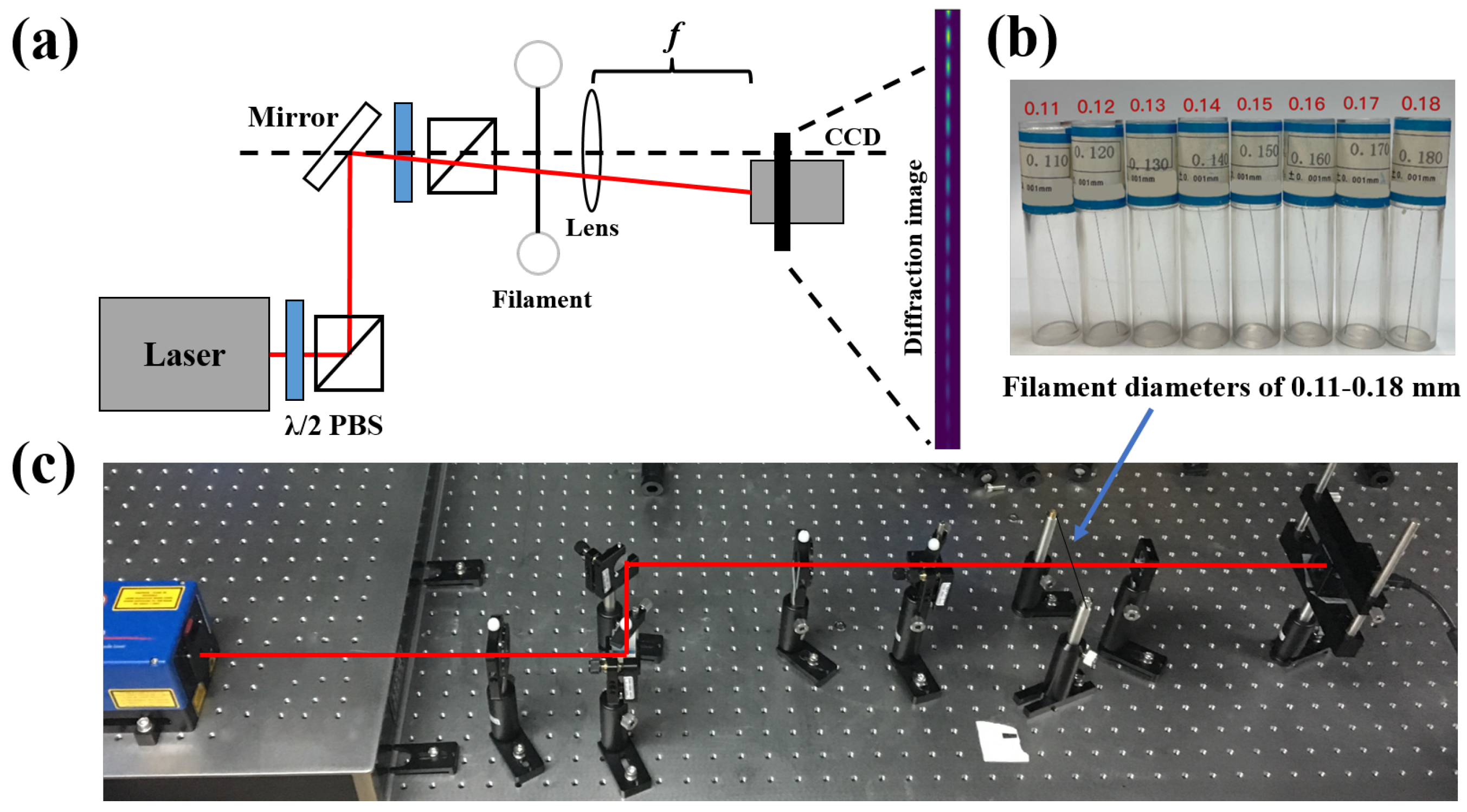
3.1. Experiments

The diagram of experimental setup is shown in Figure 1a. We used two polarization beam splitters (PBS) to adjust the laser intensity to prevent saturation of the laser intensity at the incident CCD. In our experiments, we chose a wavelength of 780.24 nm (The choice of laser needs to satisfy: the laser is coherent light; the wavelength should be in the response range of the CCD). Some of the filaments are shown in Figure 1b. A photograph of the experimental setup is shown in Figure 1c.
To assess the measurement accuracy and measurement range, diffraction images were acquired for filaments of different diameters and different focal lengths (as shown in Table 1). Multiple sets of images were taken at different laser intensities for each diameter of filament in the Table 1. A selection of common lenses with different focal lengths was used for comparison ( f = 75 mm and f = 120 mm of convex lenses), so that the reliability of the measurement method can be tested. The filaments of 125 ± 0.1   μ m and 125.2 ± 0.1   μ m diameter have a relatively high accuracy, with an accuracy of 0.1 μ m arising from mechanical processing. This group of filaments can therefore be applied to assess the accuracy of measurements. Furthermore, the filament diameter of 125.2 μ m was chosen to compare the different fitting methods. Several diffraction images of this filament were taken, and the results of each were analyzed for errors. Finally, to evaluate the measurement range of the method and to verify the stability of the measurements with different diameters, filaments of 110–180 ± 1 μ m diameter are measured, and the results are compared with the results of different fitting algorithms.

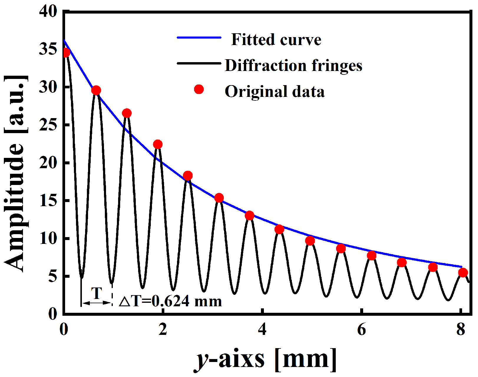
3.2. Methods of Image-Based Fitting
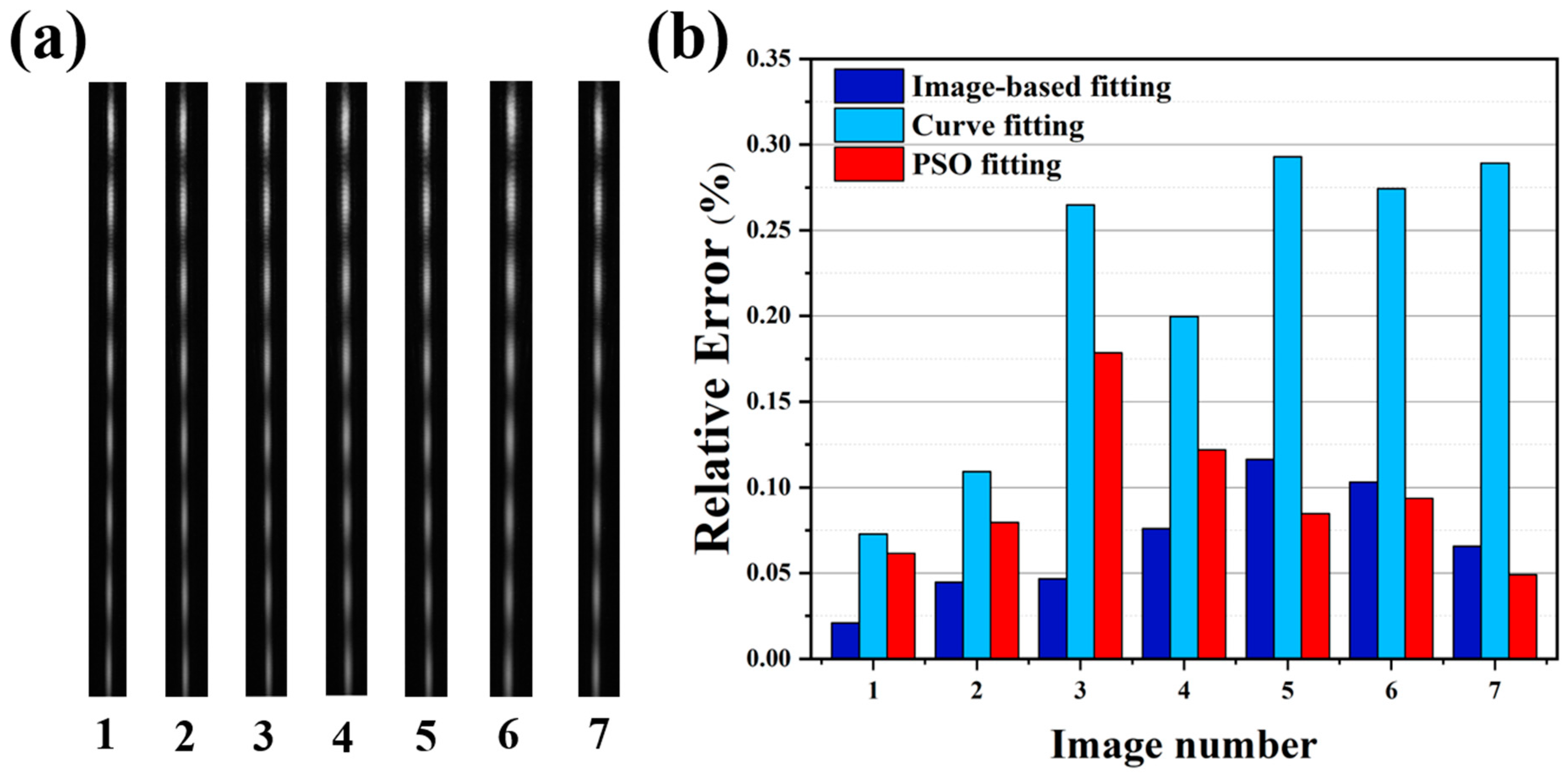
Image processing and image-based fitting steps are shown in Figure 2. Firstly, when diffraction images are taken through the CCD, it is necessary to avoid the laser intensity being so strong that the pixel cells become saturated. Then, diffraction images are rotated and cropped to easily evaluate the orientation of fringes on the CCD plane. The Gaussian low-pass filtering and gamma correction are applied to the image to give more realistic diffraction information. Then, the initial parameters of the fit are extracted mathematically. Finally, the measuremental results are obtained by fitting the diffraction image.
When fitting the diffraction image, the direction of diffraction fringes on the image should be taken into account. In that case, the coordinate system of the image can be converted to the coordinate system of diffraction fringes. Equations of the coordinate transformation are as follows:
x = X × d cos θ Y × d sin θ y = X × d sin θ + Y × d cos θ .
where d is the pixel size, θ is the rotation angle of the fringe on the imaging surface, and X , Y are the x-axis and y-axis pixels of the image plane.
The initial parameters are estimated through physical and mathematical methods, which can improve the accuracy of measurements and calculation speed. The estimation of the initial parameter of θ can be set to zero by rotating the fringe image. For the estimation of initial parameter x 0 , the imaging matrix can be changed, and the fringe image is cropped to ensure that the fringe is at the image center x 0 = x m a x / 2 (as shown in Figure 1). The initial value ( I 0 200 , c 0 ) can be given according to the gray value of the image; ω p is the estimated value ( ω p 1.9 × 10 3 ). The estimation of y 0 is more important, and its accuracy directly affects the measuremental accuracy of diameters. From the diffraction fringes, it can be found (as shown in Figure 3) that the extreme points of each bright fringe satisfy the mathematical relation as diffractive fringes. This satisfied equation is as follows:
y n = I s ( π ( y y 0 + 1 2 ) ) 2 + I b i a s ,
where I s and I b i a s represent the laser intensity and background of intensity, respectively; y 0 can be obtained by fitting Equation (5).
The initial value b of filament diameter is calculated by λ f / Δ T d ; Δ T is the average period of fringe. Each image is brought into the model for calculation, and an estimated initial parameter can be output by using the method described above. The initial parameters are then taken and brought into the fitting equation for optimization. Ultimately, the optimal solution for fitting parameters is obtained.
In the fitting process, the initial values of fitting parameters and the optimization algorithm are important factors in determining the final results of the fit. In the method, the LM algorithm (local optimization algorithm) is employed to solve the fitted parameters, which often results in a locally optimal solution, leading to possible errors in the fitting results. Therefore, a comparison was made with the Particle Swarm Optimisation (PSO) algorithm (global optimisation algorithm) [19]. The objective optimization algorithm of these two methods is the sum of squares of errors ( min R = i , j m , n ( I i , j I ˜ i , j ) 2 / m n ). In the calculation, the method of the LM algorithm requires initial parameters for the fit. The PSO fitting method does not require initial parameters, but the effectiveness of the fit is proportional to the time.

4. Results

Filament diameters of 100–200 μ m are chosen for the measurements, which is close to the core of an optical fiber. This is because the device can be applied in the future for core measurements of optical fibers.
In the experiment, filaments of different diameters ( b = 125 ± 0.1   μ m and b = 125.2 ± 0.1   μ m) are measured at two focal lengths, which are f = 75 mm and f = 120 mm (the results shown in Table 2). Each group of filaments and lenses are measured several times at different laser intensities. From the results, the measured diameter values deviate by less than 0.2 μ m relative to the actual diameter at different focal lengths. Multiple measurements are made on filaments of diameter 125 μ m and 125.2 μ m, with a standard deviation (STD) of less than 0.13 μ m (The maximum relative standard deviation (RSD) is 0.1%). As a result, filament diameters can be measured with an accuracy of approximately 0.2 μ m in practical experiments.
To be able to compare the results of different methods for the same filament diameter, a 125.2 μ m diameter filament is selected for the experiment. Figure 4a shows diffraction images of a filament with a diameter of 125.2 μ m. The absolute errors of measurement for the different methods are shown in Figure 4b. According to the results, the method of image-based fitting has better stability in the calculation. Its accuracy is superior to the fringe fitting of the fringes. The PSO fitting method requires adjustment of the particle parameters and long convergence times (Each calculation takes approximately half an hour), which results in more unstable PSO fitting results compared to image-based fitting. In addition, each initial parameter can be calculated mathematically without artificial input in the calculation. This allows the parameter optimization process to converge quickly, with each calculation taking less than one minute.
Theoretically, measurements can be obtained, and diffraction images of filaments have a significant periodicity. However, the number of periods has a definite influence on image-based fitting. The accuracy of measurements will vary for different diameters of the filament. In experiments, 0.11–0.18 μ m diameter filaments are selected for measurement so that the measurement accuracy of different diameter filaments could be compared. The results are shown in Table 3. The deviation in the filament diameter obtained with the image-based fitting is within 1 μ m of the filament calibration value. In addition, the standard deviation of measurement is less than 0.20 μ m for each set of filaments. In summary, these demonstrate that the method is more accurate in these filaments compared to other methods.
In the experiment, the filtering effect of the image has an impact on the accuracy of the method. The parameters of filter and Gamma correction need to be adjusted at different laser intensities. In summary, the signal-to-noise ratio (SNR) after image processing is greater than 35, and the relative error of measurement will be less than 0.12%.

5. Discussion

5.1. Analysis of Accuracy

The accuracy of the model fit measurements was assessed by error analysis. The complete fitting equation can be obtained by bringing Equation (3) into Equation (8), which is more complex. Simplifications have been made to facilitate the analysis of the errors caused by each parameter. To easily analyze the errors caused by each parameter, we will only analyze the effect of each parameter on the period of the diffraction fringe. The expression for a diffraction fringe period in Equation (3) is as follows:
π y T = π b d ( X sin θ + Y cos θ ) λ f ,
where T is the length of the period of fringe. In the experiments, θ is approximately equal to zero, and we simplify Equation (4) to obtain the period expression ( T λ f / b d cos θ ). Based on this equation, the standard deviation transfer equation is as follows:
σ b = σ λ b λ + σ θ b θ + σ T b T + σ d b d + σ f b f = σ λ f sec ( θ ) d T + σ θ f λ tan ( θ ) d T cos ( θ ) + σ T f λ sec ( θ ) d T 2 + σ d f λ sec ( θ ) d 2 T + σ f λ sec ( θ ) d T .
The specific parameters of our experiments are brought into Equation (7) to estimate the theoretical standard deviation (f = 120 mm, d = 4.8 μ m, λ = 780.24 nm, T = 156.04 pixels, θ = 0.01 rad). For the experiments, the accuracy of the laser wavelength ( λ ) is about 0.01 nm, which has almost no influence on the final measurement results. During imaging, the fringe is recognized in images by the algorithm and rotated to a vertical direction so that the accuracy of angle ( θ ) is approximately 0.005 rad. The diffraction fringe period (T) of a 125 μ m diameter filament averages about 156.04 with an accuracy of about 0.1. The size accuracy of the CCD pixel (d) is 10 nm. The focal length (f) is measured with an accuracy of about 0.1 mm, both of which are calculated to have the greatest influence on the measurement accuracy. In the theoretical, the accuracy of the diameter measurements is about 0.36 μ m.
However, measurement accuracy can be further improved by increasing the measurement accuracy of the focal length and the size accuracy of the CCD pixels. Firstly, the image can be interpolated to compensate for the pixel size accuracy, and the accuracy of the period length can be reduced to 0.05. Secondly, it is difficult to improve the accuracy of the focal length measurement because the imaging surface may not be at the focal point of the lens. To solve this problem, we measured the focal length with a calibration method. The focal length is measured with an image-based fitting based on a high accuracy filament, which allows an accuracy of 0.01 mm to be achieved. With these methods, the theoretical accuracy of the diameter measurement can be achieved to 0.2 μ m.

5.2. Improvement of the Fitted Equation

In practice, the position of the CCD may not be in the focal point of the lens. Equation (3) can be replaced as follows:
I = I 0 π ( Erf [ ( 1 i ) ( b ( L f ) 2 f ( y y 0 ) ) / 4 L ( L f ) f / k ] + Erf [ ( 1 i ) ( b ( L f ) + 2 f ( y y 0 ) ) / 4 L ( L f ) f / k ] ) ( Erf [ ( 1 + i ) ( b ( L f ) 2 f ( y y 0 ) ) / 4 L ( L f ) f / k ] + Erf [ ( 1 + i ) ( b ( L f ) + 2 f ( y y 0 ) ) / 4 L ( L f ) f / k ] ) exp [ ( x x 0 ) 2 w p 2 ] / 2 k ( 1 f 1 L ) + c ,
where L is the actual position of the imaging surface, k = 2 π cos ( ( y y 0 ) / L ) / λ is the wave vector of the laser. The spacing between the position of the image plane and the focal length of the lens is ( L f ) . In the calculation, Equation (3) or Equation (8) can be used to fit the fringe image. Before the diameter is calculated with the physical model, it is essential to measure or calibrate the value of f(Equation (8)) or L(Equation (8)). In our experiment, we used the exact filament diameter to calibrate the two parameters. The two models actually measured essentially the same result. However, Equation (8) is theoretically more suitable as a fitted equation.

6. Conclusions

This paper proposes a method for measuring filament diameter based on an image-based fitting. The method covers the processing of diffraction images and the extraction of fitting parameters. The method improves the accuracy of the measurement by direct fitting to an image, which retains most of the diffraction information. To verify the accuracy of this method, two standard filaments with nominal values of 125 ± 0.1   μ m and 125.2 ± 0.1   μ m were measured, and the relative measurement errors of this method are less than 0.12%. Then, we have compared the method with the PSO fitting method and the fringe fitting method. The results indicated that the accuracy of the method is better than both methods. In addition, to assess the measurement range and the stability of the method, filaments of 110–180 μ m diameter were chosen for measurement. The standard deviation of measurements is less than 0.2 μ m, and the RSD of measurements is less than 0.14%. In conclusion, this method makes the fitting results more accurate as it solves the problem of the image and the extraction of the parameters. Compared to the PSO-based fitting, this method is faster in terms of computational speed. In summary, the accuracy of this method is proven in the measurement results, and it can be used for high accuracy diameter measurements.

Author Contributions

Conceptualization, Y.Z.; data curation, Y.Z. and Y.L., B.W.; formal analysis, Y.Z. and B.W.; funding acquisition, Q.L., Z.H.; investigation, Y.Z. and B.W.; methodology, Y.L. and Y.Z., B.C.; diffraction devices, Y.Z.; Q.L., D.L. and F.W.; resources, Y.Z. and B.C.; software, Y.Z., B.C.; validation, Y.Z., F.W.; writing—original draft, Y.Z.; Y.L. writing—review and editing, Y.Z. and B.W., Q.L. All authors have read and agreed to the published version of the manuscript.

Funding

This work was supported by the Research and application experiment of carrying measurement and support technology for ocean route (DD2021085); National Natural Science Foundation of China (NSFC) (61727821, 61475139, 11604296); Space Exploration Program and the Qian Xuesen Laboratory, China Academy of Space Technology (TKTSPY-2020-06-01).

Institutional Review Board Statement

Not applicable.

Informed Consent Statement

Not applicable.

Data Availability Statement

The data presented in this study are available on request from the corresponding author.

Acknowledgments

The authors are grateful to other colleagues for their help during the period of experimental measurement.

Conflicts of Interest

The authors declare no conflict of interest.

References

  1. Ma, Z.; Merkus, H.G.; de Smet, J.G.; Heffels, C.; Scarlett, B. New developments in particle characterization by laser diffraction: Size and shape. Powder Technol. 2000, 111, 66–78. [Google Scholar] [CrossRef]
  2. Agrawal, Y.; Whitmire, A.; Mikkelsen, O.A.; Pottsmith, H. Light scattering by random shaped particles and consequences on measuring suspended sediments by laser diffraction. J. Geophys. Res. Ocean. 2008, 113, C4. [Google Scholar] [CrossRef] [Green Version]
  3. Richter, C.; Zschornak, M.; Novikov, D.; Mehner, E.; Nentwich, M.; Hanzig, J.; Gorfman, S.; Meyer, D.C. Picometer polar atomic displacements in strontium titanate determined by resonant X-ray diffraction. Nat. Commun. 2018, 9, 1–9. [Google Scholar] [CrossRef] [PubMed] [Green Version]
  4. Khodier, S.A. Measurement of wire diameter by optical diffraction. Opt. Laser Technol. 2004, 36, 63–67. [Google Scholar] [CrossRef]
  5. Couto, H.J.; Nunes, D.G.; Neumann, R.; França, S.C. Micro-bubble size distribution measurements by laser diffraction technique. Miner. Eng. 2009, 22, 330–335. [Google Scholar] [CrossRef]
  6. Fisher, P.; Aumann, C.; Chia, K.; O’Halloran, N.; Chandra, S. Adequacy of laser diffraction for soil particle size analysis. PLoS ONE 2017, 12, e0176510. [Google Scholar] [CrossRef] [PubMed] [Green Version]
  7. Wu, Y.; Ma, J.; Yang, Y.; Sun, P. Improvements of measuring the width of Fraunhofer diffraction fringes using Fourier transform. Optik 2015, 126, 4142–4145. [Google Scholar] [CrossRef]
  8. Demeyere, M.; Eugène, C. Measurement of cylindrical objects by laser telemetry: A generalization to a randomly tilted cylinder. IEEE Trans. Instrum. Meas. 2004, 53, 566–570. [Google Scholar] [CrossRef]
  9. Bernabeu, E.; Serroukh, I.; Sanchez-Brea, L.M. Geometrical model for wire optical diffraction selected by experimental statistical analysis. Opt. Eng. 1999, 38, 1319–1325. [Google Scholar] [CrossRef]
  10. Li, C.T.; Tietz, J.V. Improved accuracy of the laser diffraction technique for diameter measurement of small fibres. J. Mater. Sci. 1990, 25, 4694–4698. [Google Scholar] [CrossRef]
  11. Yang, S.; Chen, B.; Lin, B.; Cao, X. Filament diameter measurement system based on dual diffraction. Chin. Opt. Lett. 2015, 13, 120501. [Google Scholar] [CrossRef]
  12. Khajornrungruang, P.; Kimura, K.; Suzuki, K.; Inoue, T. Micro tool diameter monitoring by means of laser diffraction for on-machine measurement. Int. J. Autom. Technol. 2017, 11, 736–741. [Google Scholar] [CrossRef]
  13. Gavin, H.P. The Levenberg-Marquardt Algorithm for Nonlinear Least Squares Curve-Fitting Problems; Department of Civil and Environmental Engineering, Duke University: Durham, UK, 2020. [Google Scholar]
  14. Liu, Q.; Wei, F. Research on the Dark Stripes Extraction Algorithm for Measuring Diameter with Diffraction. Opt. Photonics J. 2013, 3, 53–56. [Google Scholar] [CrossRef] [Green Version]
  15. Elfurjani, S.; Bayesteh, A.; Park, S.; Jun, M. Dimensional measurement based on rotating wire probe and acoustic emission. Measurement 2015, 59, 329–336. [Google Scholar] [CrossRef]
  16. Pritchett, T.M.; Trubatch, A.D. A differential formulation of diffraction theory for the undergraduate optics course. Am. J. Phys. 2004, 72, 1026–1034. [Google Scholar] [CrossRef]
  17. Born, M.; Wolf, E. Principles of Optics: Electromagnetic Theory of Propagation, Interference and Diffraction of Light; Elsevier: Amsterdam, The Netherlands, 2013. [Google Scholar]
  18. Hecht, E. Optics, 5e; Pearson Education India: Delhi, India, 2002. [Google Scholar]
  19. Kundu, R.; Das, S.; Mukherjee, R.; Debchoudhury, S. An improved particle swarm optimizer with difference mean based perturbation. Neurocomputing 2014, 129, 315–333. [Google Scholar] [CrossRef]
Figure 1. Experimental setup for diffraction measurements: (a) the diagram of the experimental setup; polarization beam splitters (PBS) are used to adjust the laser intensity, f is the focal length of the lens, the wavelength of laser is 780.24 nm, and λ / 2 is the half-wave plate, the pixel size of CCD (MV-CA050-20UM) is 4.8 μm, and the resolution of CCD is 2592 × 2048; (b) some of the actual filaments; (c) actual photograph of the diffraction setup.
Photonics 09 00556 g001
Figure 2. The detailed descriptions diagram of the method: (a) the procedure for fitting diffraction images; (b) diffraction images with filtering and gamma correction.
Photonics 09 00556 g002
Figure 3. Fitting of extreme value points for the diffraction fringe. The black curve is the diffraction fringe; the red spots are the laser intensity extremums; the blue curve is the extremum fit curve.
Photonics 09 00556 g003
Figure 4. Measured results for the filament diameter of 125.2 ± 0.1 μ m: (a) diffraction images of a 125.2 μ m diameter filament at a focal length (f) of 120 mm; (b) measured results of 125.2 μ m filaments with different methods.
Photonics 09 00556 g004
Table 1. Diffraction images of different filaments * (unit: μ m).
Focal length
75 mm
Photonics 09 00556 i001 Photonics 09 00556 i002 Photonics 09 00556 i003 Photonics 09 00556 i004
Filament diameter125.2125.2125.0125.0
Focal length
120 mm
Photonics 09 00556 i005 Photonics 09 00556 i006 Photonics 09 00556 i007 Photonics 09 00556 i008
Filament diameter125.2125.2125.0125.0
Focal length
126.2 mm
Photonics 09 00556 i009 Photonics 09 00556 i010 Photonics 09 00556 i011 Photonics 09 00556 i012 Photonics 09 00556 i013 Photonics 09 00556 i014 Photonics 09 00556 i015 Photonics 09 00556 i016
Filament diameter110120130140150160170180
* Multiple images were taken for each filament diameter.
Table 2. Actual measurement results (unit: μ m).
DiameterAverage of
Measurements
Standard
Deviation
Relative Standard
Deviation (%)
Absolute ErrorRelative Error
(%)
125.00 ± 0.1  1 125.060.130.100.060.05
125.20 ± 0.1125.160.100.080.040.03
125.00 ± 0.1  2 124.860.030.020.140.11
125.20 ± 0.1125.350.040.030.150.12
1 The focal length of the lens is 120 mm. 2 The focal length of the lens is 75 mm.
Table 3. Comparison of different methods * (unit: μ m).
DiameterResults of Image-Based FittingRSD (%)Results of Fringe FittingRSD (%)Results of PSO FittingRSD (%)
110 ± 1110.51
(STD = 0.07)
0.06113.73
(STD = 1.58)
1.38110.6
(STD = 2.30)
2.08
120 ± 1119.52
(STD = 0.12)
0.10118.13
(STD = 1.57)
1.33119.80
(STD = 0.07)
0.06
130 ± 1129.24
(STD = 0.06)
0.05131.37
(STD = 0.78)
0.59129.28
(STD = 0.08)
0.06
140 ± 1139.95
(STD = 0.20)
0.14141.48
(STD = 0.43)
0.30139.62
(STD = 0.23)
0.16
150 ± 1150.27
(STD = 0.01)
0.01151.87
(STD = 0.23)
0.15149.83
(STD = 0.20)
0.15
160 ± 1159.19
(STD = 0.09)
0.01158.85
(STD = 0.77)
0.48159.45
(STD = 1.14)
0.71
170 ± 1169.68
(STD = 0.11)
0.06172.19
(STD = 0.23)
0.13169.54
(STD = 0.09)
0.05
180 ± 1180.47
(STD = 0.05)
0.03180.13
(STD = 0.99)
0.55180.16
(STD = 0.30)
0.16
* The focal length after calibration is 126.22 mm.
Publisher’s Note: MDPI stays neutral with regard to jurisdictional claims in published maps and institutional affiliations.

