Analysis of Scintillation Effects on Free Space Optical Communication Links in South Africa

Abstract

The performance of free space optical communication (FSOC) systems is severely degraded by certain atmospheric conditions prevalent in places where they are deployed, in spite of their numerous advantages. In clear weather conditions, the random fluctuation in the atmosphere’s refractive index causes substantial scintillation losses to transmitted optical signals. It is therefore imperative to estimate the potential losses due to atmospheric turbulence in locations where FSOC links are to be deployed. This will provide the necessary fade margin for FSOC systems so that designed links withstand such atmospheric disturbances. In this paper, statistical analysis of wind speed data collected for various cities of South Africa is used for calculating the corresponding refractive index structure parameter (${{\displaystyle C}}_n^2$). These ${{\displaystyle C}}_n^2$ values, as well as the zero inner scale and infinite outer scale model and finite inner and finite outer scale model, are used in computing the scintillation indices not exceeding 50%, 99%, 99.9%, and 99.99% of the time for the investigated locations. The Lognormal and Gamma–gamma distribution models are then employed for the computational analysis of the irradiance fluctuations and channel characteristics while considering the effect of pointing errors for weak and moderate to strong turbulence regimes. Finally, derived mathematical expressions for outage probabilities and bit error rate (BER) performances for FSOC links, employing various intensity modulation and direct detection (IM/DD) schemes, are presented.

1. Introduction

The International Mobile Telecommunications 2020 (IMT-2020) specifications, developed by the third generation partnership project (3GPP) for new radio (NR) operations in the fifth generation (5G) spectrum, is expected to accomplish the following performance requirements: ultra-reliable and low latency communications (URLLC) in the user plane as low as 1 ms; massive machine type communications (mMTC) that support up to 1 million devices per square km; and enhanced mobile broadband (eMBB) with uplink and downlink speeds of up to 10 and 20 Gbits/s [1,2]. These technical requirements are needed for the high bandwidth demands of augmented reality (AR), virtual reality (VR), and mixed reality (MR) applications, as well as the seamless and optimal functionality of Massive Internet of Things (MIoT) and Vehicle-to-Everything (V2X) connections for the smooth running of emerging smart cities [3,4,5].

Free space optical communication (FSOC), whether as a standalone or hybrid technology, is a promising complementary solution platform for 5G backhaul networks [6]. FSOC systems convey bidirectional information at high data rates through the atmosphere between line-of-sight (LOS) optical transceivers. Their numerous advantages include: very high throughput, highly secure transmission, relatively low cost, and ease of deployment when compared to the rigours encountered in the installation of fibre-optic infrastructures, high resistance to signal eavesdropping, and low latency communication since the velocity of light in the atmosphere is about 40% faster than in the fibre-optic cable [7,8]. In spite of these advantages, the performance of FSOC systems is severely affected by atmospheric impairments.

Dense fog, haze, and snow storms are known to cause the aerosol scattering of optical signals and consequently degrade the availability of FSOC links [9]. In clear weather, atmospheric turbulence or scintillation is the most significant cause of impairment in received signal quality [10]. Atmospheric turbulence causes fluctuations in air temperature, pressure, density, and humidity, which results in rapid variations in the atmosphere’s refractive index. The impact of these changes leads to irradiance fluctuations of received information signals [11]. Other turbulence effects on FSOC link performance are disruptions in the coherence of the laser beam and distortions in the optical wave front. Optical wave front distortions result in laser beam broadening, uneven beam energy redistribution within a cross-section of the laser, and beam wander [12]. Improving the bit error rate (BER) performance of FSOC systems during these adverse weather situations is the major challenge in the design of FSOC links [13].

In addition, the misalignment between FSOC transceivers cause pointing errors, which increase the performance degradation of FSOC links. These misalignments arise from either mechanical vibrations in the system as a result of wind or building movement or errors in the tracking system. The displacement of the laser beam along vertical (elevation) and horizontal (azimuth) directions, which are generally expected to be independent Gaussian random variables, result in pointing errors [14,15,16,17,18,19]. Beam width, boresight, and jitter are the three fundamental components of a pointing error. The beam width is the beam waist (radius computed at e⁻²), while the jitter is the random offset of the beam centre at the detector plane produced by building motion, minor earthquakes, and dynamic wind loads. The boresight denotes the fixed displacement between the beam centre and the alignment point. It should be noted, however, that boresight displacements are of two kinds: inherent boresight displacement and additional boresight error. The first is related to the spacing between the detector’s receive apertures. This inherent boresight displacement corresponds to a fixed distance, namely the distance between each received aperture and its associated alignment point. The second is related to the boresight error caused by the building’s thermal expansion [14,15,16,17,18,19].

Conventionally, FSOC systems employ intensity modulation/direct detection (IM/DD) schemes. Most commercial FSOC links are based on the on-off keying (OOK) modulation schemes due to their low cost and simple implementation. However, FSOC systems employing OOK require adaptive thresholding, which is difficult to implement when combating irradiance fading, hence their sub-optimal performance over atmospheric turbulence channels [11,13,20]. Binary phase-shift keying subcarrier intensity modulation (BPSK-SIM) FSOC systems have also been investigated extensively. In spite of their superior BER performance when compared with other coherent and non-coherent modulation schemes, BPSK-SIM FSOC links have poor power efficiency when compared to pulse position modulation (PPM) FSOC links [20,21]. FSOC systems employing sub-carrier intensity quadrature amplitude modulation (SIM-QAM) have also been investigated. SIM-QAM FSOC links are found to have better spectral efficiency compared to PPM FSOC links which exhibit poor bandwidth performance. SIM-QAM FSOC systems have great potential for future FSOC systems since they deliver a higher data rate without an increase in the required bandwidth due to their inherent attribute of transmitting more bits per symbol [11,22,23,24].

Between April 2015 and February 2016, the First European South African Transmission ExpeRiment (FESTER) was conducted in False Bay, South Africa, to study the influence of atmospheric turbulence on wave propagation [25,26]. The experiment focused on measuring and modelling optical turbulence, electro-optical system performance, and imaging. Despite the fact that wind direction, wind speed, and the kinematic vertical sensible heat flux all have an effect on optical turbulence, thermal forces were found to have the greatest impact on it, with both exhibiting a direct relationship regardless of the seasons. Additionally, it was discovered that as friction velocity increases, optical turbulence increases. Onshore and offshore wind directions produced differences in the turbulence strength. With onshore conditions during the winter, the turbulence strength is extremely low. Spring brings an increase in the variability of turbulence strength. The highest refractive index structure parameter (${{\displaystyle C}}_n^2$) values above 10⁻¹⁴ m^−2/3 may be reached during the summer [25,26].

The ${{\displaystyle C}}_n^2$, which is also dependent on the root-mean-square (RMS) wind speed and altitude of a location, is used to characterize atmospheric turbulence as weak, moderate or strong at any point in time [27,28,29,30]. Most of the results obtained in literature [6,10,11,12,13,20,23,31,32,33] assume arbitrary ${{\displaystyle C}}_n^2$ values or estimate them based on average wind speed measurements for a particular location. In some cases, worst case scenarios of atmospheric turbulence based on the maximum values of wind speed are investigated [29,33]. However, these measurements are based on data spanning less than 4 years. As a result, they cannot be accurately used to estimate the maximum attenuation due to turbulence-induced irradiance fading. In this paper, the focus is placed on the wind distributions based on data spanning over 8 years for the various locations of interest where FSOC links are to be deployed. This will allow for accurate estimation of the ${{\displaystyle C}}_n^2$, and consequently, correct calculations of the maximum attenuation due to turbulence, and the performance of various FSOC links during such periods.

Therefore, the key contributions of this work are as follows:

• Computation of the scintillation profile for Gaussian beam FSOC signals in the nine cities under investigation based on the zero inner scale and infinite outer scale model and finite inner and finite outer scale model. To the best of our knowledge, the computation of the scintillation profile for Gaussian beam FSOC links transmitting at 1550 nm in the cities of interest, while considering periods not exceeded 50%, 99%, 99.9%, and 99.99% of the time have not been reported in open literature.
• Aerosol scattering losses over various distances for FSOC links transmitting at 1550 nm with respect to events not exceeded 50%, 99%, 99.9%, and 99.99% of the time, for nine major locations in South Africa, are investigated.
• Outage probabilities of Gaussian beam FSOC links based on the aforementioned scintillation models, while taking into account the effect of pointing errors for events not exceeding the previously mentioned time intervals, are presented for various locations of interest.
• Analysis of the bit error rate (BER) performance for intensity modulation and direct detection (IM/DD) avalanche photodiode (APD) FSOC systems transmitting at 1550 nm and based on OOK, BPSK, square, and rectangular SIM-QAM schemes during weak, moderate, and strong atmospheric turbulence, with regards to average weather measurements and events not exceeding 99%, 99.9%, and 99.99% of the time are presented.

The rest of this paper is organized as follows: Section 2 presents the ground wind speed distributions for nine cities in South Africa; Section 3 presents and analyses the modified Rytov theory based on zero inner scale and infinite outer scale model and finite inner and finite outer scale model for Gaussian beam waves. Section 4 presents aerosol scattering losses over various link distances for the nine cities under investigation. Weak, moderate, and strong atmospheric turbulence parameters during clear weather for the locations of interest based on the Lognormal and Gamma–gamma turbulence models are provided in Section 5, while outage probability analysis of FSOC links with respect to the effect of pointing errors is presented in Section 6. In Section 7, the average BER analysis, taking in account pointing error effects for various FSOC systems in weak, moderate, and strong turbulence regimes is derived and the results are analysed, while conclusions are provided in Section 8.

2. Wind Speed Distribution

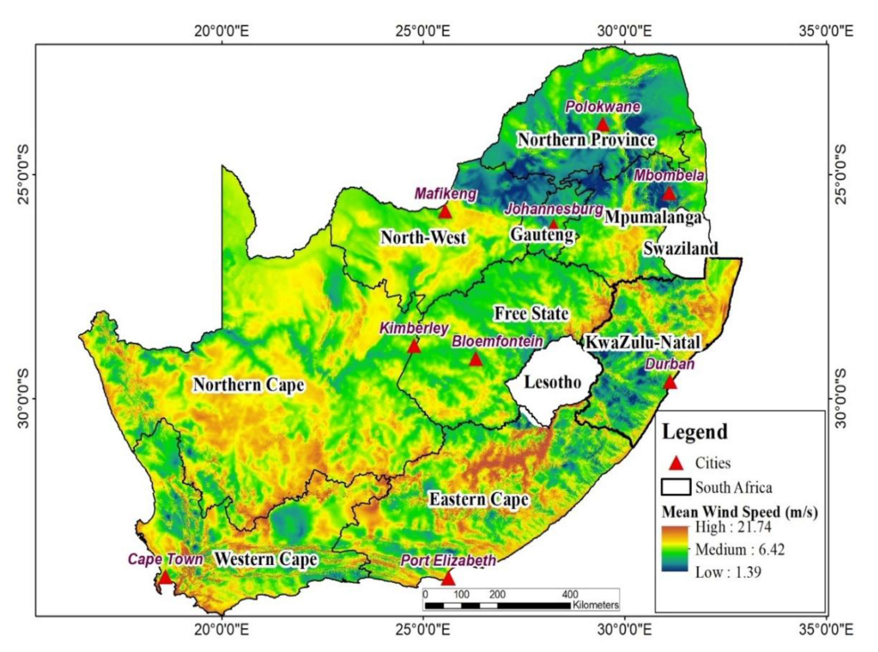
Figure 1 shows the map of South Africa depicting the average wind speed (m/s) at 100 m above ground level for selected cities investigated in this work. The average wind speed data used in plotting Figure 1 spans January 2008 until December 2017 and was sourced from [34]. The data in Figure 1 is very similar to the average measurement values presented in Table I of [10,32]. Wind speed data from January 2010 until June 2018 was also acquired from the South Africa Weather Service (SAWS) for major locations in each of the nine provinces of South Africa. The data was collected hourly for the 8½ year period. The locations of interest investigated in this work are: Bloemfontein, Cape Town, Durban, Johannesburg, Kimberley, Mafikeng, Mbombela, Polokwane, and Port Elizabeth. The data provided by the SAWS, which was collected from various weather stations placed a few meters above the ground, was statistically processed and used for all our computations in this work.

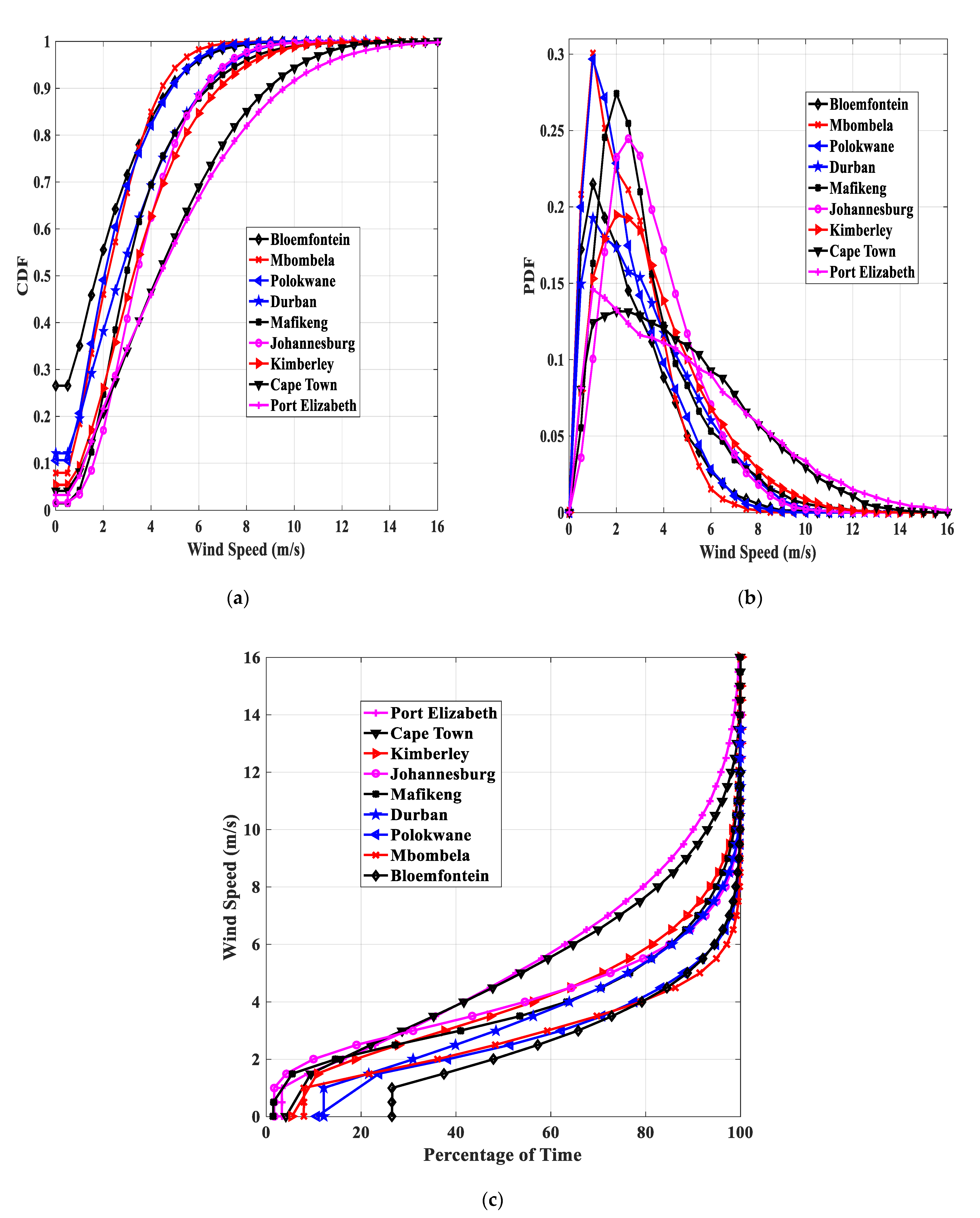
Figure 2a–c, alongside all other analysis done in this work, are based on the measurement data obtained from the SAWS. Figure 2a shows the CDF of wind speed for various cities in South Africa, while Figure 2b presents the PDF of wind speed for the same locations. In Figure 2a, the coastal cities of Port Elizabeth and Cape Town have the highest probabilities of occurrence of high wind velocities compared to other cities in South Africa. The cities of Bloemfontein, Mbombela, and Polokwane have the highest likelihood of occurrence of low wind speeds. In Figure 2b, the probability of occurrence of wind speeds of 1 m/s in the cities of Mbombela and Polokwane is ~0.3, while the cities of Cape Town and Port Elizabeth have the lowest likelihood of occurrence (less than 0.15) of low wind velocities when compared with other cities in South Africa. Figure 2c shows the wind speed exceedance against the percentage of time for the various locations of interest. Figure 2c validates the results in Figure 2a,b.

Wind velocities greater than 4 m/s occur ~60% of the time in the cities of Port Elizabeth and Cape Town, while in Polokwane, Mbombela, and Bloemfontein, wind speeds higher than 4 m/s occur less than 25% of the time.

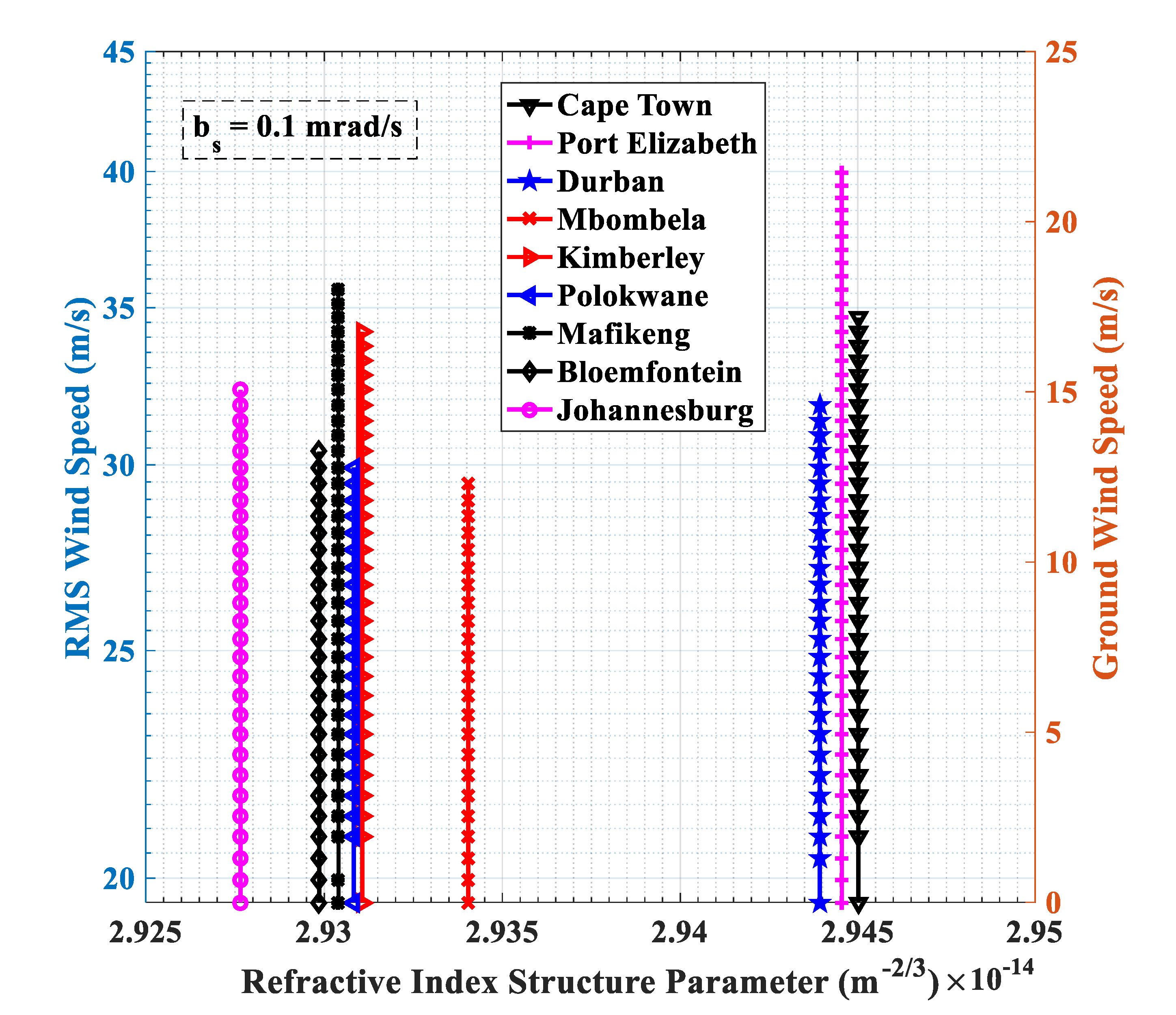
The ${{\displaystyle C}}_n^2$ in m^−2/3 based on the Hufnagel–Andrews–Phillips (HAP) model is presented in [35,36,37] as:

$${{\displaystyle C}}_n^2\left(a\right)=M\left[\frac{297}{5\times {{\displaystyle 10}}^4}{{\displaystyle \left(\frac{{{\displaystyle W}}_{rms}}{27}\right)}}^2{{\displaystyle \left(\frac{a+{{\displaystyle a}}_s}{{{\displaystyle 10}}^5}\right)}}^{10}\exp \left(-\frac{\left(a+{{\displaystyle a}}_s\right)}{{{\displaystyle 10}}^3}\right)+\left(2.7\times {{\displaystyle 10}}^{-16}\right)\exp \left(-\frac{\left(a+{{\displaystyle a}}_s\right)}{1.5\times {{\displaystyle 10}}^3}\right)+\left(1.7\times {{\displaystyle 10}}^{-14}\right){{\displaystyle \left(\frac{{{\displaystyle a}}_o}{a}\right)}}^{-\raisebox{1ex}{$4$}\!\left/ \!\raisebox{-1ex}{$3$}\right.}\right], a>{{\displaystyle a}}_o$$

(1)

where $M$ is the scaling factor, ${{\displaystyle a}}_s$ is the reference height of the ground above sea level in metres, ${{\displaystyle a}}_o$ is the height of the first FSOC transceiver above the ground in metres, $a$ is the altitude from the reference height ${{\displaystyle a}}_o$ to the height of the other (second) FSOC transceiver above the ground in metres, and ${{\displaystyle W}}_{rms}$ is the root-mean-square (RMS) wind speed in m/s. The RMS wind speed in Equation (1) is calculated using the Bufton wind model, which is given in [35,36,38,39] as:

$${{\displaystyle W}}_{rms}=\sqrt{\frac{1}{15000}{\displaystyle \underset{5000}{\overset{20000}{\int }}{{\displaystyle \left[{{\displaystyle b}}_{s}a+{{\displaystyle W}}_g+30\exp \left(-{{\displaystyle \left(\frac{a-9400}{4800}\right)}}^2\right)\right]}}^{2}da}}$$

(2)

where ${{\displaystyle b}}_s$ is the beam slew rate associated with a satellite moving with respect to an observer on the ground in rad/s and ${{\displaystyle W}}_g$ is the ground wind speed in m/s.

The climate of South Africa is considered to be highly variable, both spatially and temporally. Spatial variations in elevation across the country contribute significantly to this variability. According to the Council for Scientific and Industrial Research’s (CSIR) Köppen–Geiger climate classification for South Africa, the country is predominantly semi-arid, with influences from temperate and tropical zones [40,41,42]. A large part of the geographical space of South Africa and Namibia is characterized by arid and hot climates, with clear skies and low annual rainfall [28,29]. Due to the similarities in the two countries’ climatic patterns, the ${{\displaystyle C}}_n^2$ based on the HAP model are expected to adequately estimate the atmospheric turbulence losses encountered by FSOC links deployed in various cities of South Africa considered in this work.

Other values where $M$ = 1, ${{\displaystyle b}}_s$ = 0.1 mrad/s, ${{\displaystyle a}}_o$ = 10 m, and $a$ = 15 m were used in computing the ${{\displaystyle C}}_n^2$ throughout this work. The altitude measurements above sea level are given in

Table 1. Reference altitude of the ground above sea level for various cities in South Africa.

City	${{\displaystyle \mathit{a}}}_{\mathit{s}} \left(\mathbf{m}\right)$
Cape Town	42
Port Elizabeth	69
Durban	106
Mbombela	865
Polokwane	1226
Kimberley	1196
Mafikeng	1281
Bloemfontein	1354
Johannesburg	1695

, and the ground wind speed data from SAWS when inserted into Equations (1) and (2) are used for determining the ${{\displaystyle C}}_n^2$ of the various locations shown in Figure 3.

3. Modified Rytov Theory for Gaussian Beam Waves

Fluctuations in the wind speed and atmospheric temperature generate unstable air masses that eventually break up into turbulent eddies or cells of varying scale sizes with constant ${{\displaystyle C}}_n^2$. These inhomogeneities vary in size from macroscale to microscale, and are of different densities [12]. As the Gaussian beams transverse the free space channel, these zones of turbulent air motion act as lenses that scatter the beams off their intended paths. The microscale eddies ${{\displaystyle l}}_o$, also known as the inner scale of turbulence, are approximately 3 to 10 mm near the ground. The macroscale eddies ${{\displaystyle L}}_o$, also referred to as the outer scale of turbulence, are in the range of several metres above the ground level. Optical turbulence is primarily defined by ${{\displaystyle C}}_n^2$, ${{\displaystyle l}}_o$, and ${{\displaystyle L}}_o$ [43].

3.1. Zero Inner Scale and Infinite Outer Scale Model (Infinite Kolmogorov Inertial Range)

The microscale and macroscale effects are neglected in this model. That is, ${{\displaystyle l}}_o\simeq 0$ and ${{\displaystyle L}}_o\simeq \infty$. The scintillation index or normalized irradiance variance for the zero inner scale and infinite outer scale model is expressed as [44]:

$${{\displaystyle \sigma }}_{SI}^2\left(0,L\right)=\exp \left({{\displaystyle \sigma }}_{Inx}^2+{{\displaystyle \sigma }}_{Iny}^2\right)-1$$

(3)

where ${{\displaystyle \sigma }}_{Inx}^2$ is the large-scale log–irradiance variance and ${{\displaystyle \sigma }}_{Iny}^2$ is the small-scale log–irradiance variance.

The large-scale log–irradiance variance is given as [44]:

$${{\displaystyle \sigma }}_{Inx}^2=\frac{0.49{{\displaystyle \sigma }}_B^2}{{{\displaystyle \left(1+0.56{{\displaystyle \sigma }}_B^{2.4}\right)}}^{1.167}}$$

(4)

and the small-scale log–irradiance variance is expressed as [44]:

$${{\displaystyle \sigma }}_{Iny}^2=\frac{0.51{{\displaystyle \sigma }}_B^2}{{{\displaystyle \left(1+0.69{{\displaystyle \sigma }}_B^{2.4}\right)}}^{0.833}}$$

(5)

where ${{\displaystyle \sigma }}_B^2$ is the Rytov variance for a Gaussian-beam wave, and is expressed in [38] as:

$${{\displaystyle \sigma }}_B^2\cong 3.86{{\displaystyle \sigma }}_1^2\times \left\{0.40{{\displaystyle \left({{\displaystyle \left(1+2{{\displaystyle \mathsf{\Theta }}}_1\right)}}^2+4{{\displaystyle \mathsf{\Lambda }}}_1^2\right)}}^{0.417}\times \cos \left(0.833{{\displaystyle \tan }}^{-1}\left(\frac{1+2{{\displaystyle \mathsf{\Theta }}}_1}{2{{\displaystyle \mathsf{\Lambda }}}_1}\right)\right)-0.688{{\displaystyle \mathsf{\Lambda }}}_1^{0.833}\right\}$$

(6)

where ${{\displaystyle \sigma }}_1^2$ is the Rytov variance for a plane wave, ${{\displaystyle \mathsf{\Theta }}}_1$ is the curvature parameter of the beam at the receiver, and ${{\displaystyle \mathsf{\Lambda }}}_1$ is the Fresnel ratio of the beam at the receiver. ${{\displaystyle \sigma }}_1^2$ is given as [45]:

$${{\displaystyle \sigma }}_1^2=1.23{{\displaystyle C}}_n^2{{\displaystyle k}}^{1.167}{{\displaystyle L}}^{1.833}$$

(7)

where $k$ is the wave number of the plane wave. $k$ is calculated in m⁻¹ as [45]:

$$k=\frac{2\pi }{\lambda }$$

(8)

where $\lambda$ is the wavelength in metres. ${{\displaystyle \mathsf{\Theta }}}_1$ is expressed as [46]:

$${{\displaystyle \mathsf{\Theta }}}_1=\frac{{{\displaystyle \mathsf{\Theta }}}_o}{{{\displaystyle \mathsf{\Theta }}}_o^2+{{\displaystyle \mathsf{\Lambda }}}_o^2}=1+\frac{L}{F}$$

(9)

where ${{\displaystyle \mathsf{\Theta }}}_o$ is the Beam curvature parameter at the transmitter, ${{\displaystyle \mathsf{\Lambda }}}_o$ is the Fresnel ratio of the beam at the transmitter, $L$ is the propagation distance in metres, and $F$ is the phase front radius of curvature of the beam at the receiver. ${{\displaystyle \mathsf{\Lambda }}}_1$ is given as [46]:

$${{\displaystyle \mathsf{\Lambda }}}_1=\frac{{{\displaystyle \mathsf{\Lambda }}}_o}{{{\displaystyle \mathsf{\Theta }}}_o^2+{{\displaystyle \mathsf{\Lambda }}}_o^2}=\frac{2L}{k{{\displaystyle W}}_1^2}$$

(10)

where ${{\displaystyle W}}_1$ is the beam radius in free space at the receiver. ${{\displaystyle W}}_1$ can be calculated using [43,47]:

$${{\displaystyle W}}_1={{\displaystyle W}}_o{{\displaystyle \left({{\displaystyle \mathsf{\Theta }}}_o^2+{{\displaystyle \mathsf{\Lambda }}}_o^2\right)}}^{0.5}$$

(11)

where ${{\displaystyle W}}_o$ is the beam radius at the transmitter. The beam curvature parameter at the transmitter can be expressed as [46,47]:

$${{\displaystyle \mathsf{\Theta }}}_o=1-\frac{L}{F}$$

(12)

while the Fresnel ratio of the beam at the transmitter is given as [46,47]:

$${{\displaystyle \mathsf{\Lambda }}}_o=\frac{2L}{k{{\displaystyle W}}_o^2}$$

(13)

The phase front radius of curvature of the beam at the receiver can be calculated using [38]:

$$F=\frac{{{\displaystyle F}}_o\left({{\displaystyle \mathsf{\Theta }}}_o^2+{{\displaystyle \mathsf{\Lambda }}}_o^2\right)\left({{\displaystyle \mathsf{\Theta }}}_o-1\right)}{{{\displaystyle \mathsf{\Theta }}}_o^2+{{\displaystyle \mathsf{\Lambda }}}_o^2-{{\displaystyle \mathsf{\Theta }}}_o}$$

(14)

where ${{\displaystyle F}}_o$ is the phase front radius of curvature of the beam at the transmitter.

3.2. Finite Inner and Finite Outer Scale Model (Modified Atmospheric Spectrum)

In this model, ${{\displaystyle l}}_o>0$ and ${{\displaystyle L}}_o<\infty$. The finite inner and finite outer scale effects model is actually the modified atmospheric spectrum. The scintillation index for this model can be expressed as [44]:

$${{\displaystyle \sigma }}_{SI}^2\left(0,L\right)=\exp \left({{\displaystyle \sigma }}_{Inx}^2\left({{\displaystyle l}}_o,{{\displaystyle L}}_o\right)+{{\displaystyle \sigma }}_{Iny}^2\left({{\displaystyle l}}_o\right)\right)-1$$

(15)

where

$${{\displaystyle \sigma }}_{Inx}^2\left({{\displaystyle l}}_o,{{\displaystyle L}}_o\right)={{\displaystyle \sigma }}_{Inx}^2\left({{\displaystyle l}}_o\right)-{{\displaystyle \sigma }}_{Inx}^2\left({{\displaystyle L}}_o\right)$$

(16)

The large-scale log–irradiance variance component due to the inner scale of optical turbulence is given as [44]:

$${{\displaystyle \sigma }}_{Inx}^2\left({{\displaystyle l}}_o\right)=0.49{{\displaystyle \sigma }}_1^2\left(0.333-0.5{{\displaystyle \overline{\mathsf{\Theta }}}}_1+0.2{{\displaystyle {{\displaystyle \overline{\mathsf{\Theta }}}}_1}}^2\right){{\displaystyle \left(\frac{{{\displaystyle \eta }}_x{{\displaystyle Q}}_l}{{{\displaystyle \eta }}_x{{\displaystyle +Q}}_l}\right)}}^{1.167}\times \left(1+1.75{{\displaystyle \left(\frac{{{\displaystyle \eta }}_x}{{{\displaystyle \eta }}_x{{\displaystyle +Q}}_l}\right)}}^{0.5}-0.25{{\displaystyle \left(\frac{{{\displaystyle \eta }}_x}{{{\displaystyle \eta }}_x{{\displaystyle +Q}}_l}\right)}}^{0.583}\right)$$

(17)

while the large-scale log–irradiance variance component due to outer scale of turbulence is expressed as [44]:

$${{\displaystyle \sigma }}_{Inx}^2\left({{\displaystyle L}}_o\right)=0.49{{\displaystyle \sigma }}_1^2\left(0.333-0.5{{\displaystyle \overline{\mathsf{\Theta }}}}_1+0.2{{\displaystyle {{\displaystyle \overline{\mathsf{\Theta }}}}_1}}^2\right){{\displaystyle \left(\frac{{{\displaystyle \eta }}_{xo}{{\displaystyle Q}}_l}{{{\displaystyle \eta }}_{xo}{{\displaystyle +Q}}_l}\right)}}^{1.167}\times \left(1+1.75{{\displaystyle \left(\frac{{{\displaystyle \eta }}_{xo}}{{{\displaystyle \eta }}_{xo}{{\displaystyle +Q}}_l}\right)}}^{0.5}-0.25{{\displaystyle \left(\frac{{{\displaystyle \eta }}_{xo}}{{{\displaystyle \eta }}_{xo}{{\displaystyle +Q}}_l}\right)}}^{0.583}\right)$$

(18)

where

$${{\displaystyle \overline{\mathsf{\Theta }}}}_1=1-{{\displaystyle \mathsf{\Theta }}}_1=-\frac{L}{F}$$

(19)

The nondimensional inner-scale parameter, ${{\displaystyle Q}}_l$, is calculated as [44]:

$${{\displaystyle Q}}_l=\frac{10.89L}{k{{\displaystyle l}}_o^2}$$

(20)

while the nondimensional low-pass cutoff frequency is expressed as [44]:

$${{\displaystyle \eta }}_x={{\displaystyle \left(\frac{0.38}{1-3.21{{\displaystyle \overline{\mathsf{\Theta }}}}_1+5.29{{\displaystyle {{\displaystyle \overline{\mathsf{\Theta }}}}_1}}^2}+\left(0.47{{\displaystyle \sigma }}_1^2{{\displaystyle Q}}_l^{0.167}{{\displaystyle \left(\frac{0.333-0.5{{\displaystyle \overline{\mathsf{\Theta }}}}_1+0.2{{\displaystyle {{\displaystyle \overline{\mathsf{\Theta }}}}_1}}^2}{1+2.20{{\displaystyle \overline{\mathsf{\Theta }}}}_1}\right)}}^{0.857}\right)\right)}}^{-1}$$

(21)

The artificial quantity ${{\displaystyle \eta }}_{xo}$, is defined as [44]:

$${{\displaystyle \eta }}_{xo}=\frac{{{\displaystyle \eta }}_{xo}{{\displaystyle Q}}_o}{{{\displaystyle \eta }}_{xo}{{\displaystyle +Q}}_o}$$

(22)

and the nondimensional outer-scale parameter, ${{\displaystyle Q}}_o$, is given as [44]:

$${{\displaystyle Q}}_o=\frac{64{{\displaystyle \pi }}^{2}L}{k{{\displaystyle L}}_o^2}$$

(23)

The small-scale log–irradiance variance component due to the inner scale of optical turbulence is defined as [44]:

$${{\displaystyle \sigma }}_{Iny}^2\left({{\displaystyle l}}_o\right)=\frac{0.51{{\displaystyle \sigma }}_G^2}{{{\displaystyle \left(1+0.69{{\displaystyle \sigma }}_G^{2.4}\right)}}^{0.833}}$$

(24)

where ${{\displaystyle \sigma }}_G^2$ is the Rytov variance for a Gaussian-beam wave with inner scale and is derived in [38,44].

Table 2. Average atmospheric turbulence parameters during clear weather.

City	Ground Wind Speed (m/s)	RMS Wind Speed (m/s)	$$\begin{gathered} {\mathit{C}}_{\mathit{n}}^2 \\ \left({\mathbf{m}}^{-2/3}\right) \end{gathered}$$	Propagation Length of 2 km
				Zero Inner Scale and Infinite Outer Scale Model			Finite Inner and Finite Outer Scale Model
				${\mathit{\sigma }}_{\mathit{S}\mathit{I}}^2\left(0,\mathit{L}\right)$	α	β	${\mathit{\sigma }}_{\mathit{S}\mathit{I}}^2\left(0,\mathit{L}\right)$	α	β
Johannesburg	3.8	22.85	2.9277 × 10−14	0.7488	3.3001	2.9230	0.9311	2.6207	2.5143
Bloemfontein	2.2	21.43	2.9299 × 10−14	0.7492	3.2985	2.9214	0.9317	2.6192	2.5130
Mafikeng	3.4	22.49	2.9304 × 10−14	0.7494	3.2981	2.9210	0.9318	2.6188	2.5127
Polokwane	2.5	21.70	2.9308 × 10−14	0.7494	3.2978	2.9207	0.9319	2.6185	2.5124
Kimberley	3.7	22.76	2.9311 × 10−14	0.7495	3.2976	2.9205	0.9320	2.6184	2.5123
Mbombela	2.6	21.78	2.9340 × 10−14	0.7501	3.2955	2.9183	0.9328	2.6163	2.5105
Durban	3.1	22.23	2.9439 × 10−14	0.7521	3.2884	2.9110	0.9354	2.6096	2.5047
Port Elizabeth	4.8	23.75	2.9446 × 10−14	0.7522	3.2879	2.9106	0.9356	2.6092	2.5044
Cape Town	4.7	23.66	2.9450 × 10−14	0.7523	3.2876	2.9102	0.9357	2.6089	2.5041

,

Table 3. Atmospheric turbulence parameters not exceeded 99% of the time during clear weather.

City	Ground Wind Speed (m/s)	RMS Wind Speed (m/s)	$$\begin{gathered} {\mathit{C}}_{\mathit{n}}^2 \\ \left({\mathbf{m}}^{-2/3}\right) \end{gathered}$$	Propagation Length of 1.5 km
				Zero Inner Scale and Infinite Outer Scale Model			Finite Inner and Finite Outer Scale Model
				${\mathit{\sigma }}_{\mathit{S}\mathit{I}}^2\left(0,\mathit{L}\right)$	α	β	${\mathit{\sigma }}_{\mathit{S}\mathit{I}}^2\left(0,\mathit{L}\right)$	α	β
Johannesburg	9.3	27.87	2.9277 × 10−14	0.4775	4.8389	4.4556	0.5947	3.8983	3.7156
Bloemfontein	8.0	26.67	2.9299 × 10−14	0.4778	4.8360	4.4527	0.5951	3.8957	3.7133
Mafikeng	10.5	28.99	2.9304 × 10−14	0.4779	4.8353	4.4520	0.5952	3.8951	3.7128
Polokwane	7.6	26.30	2.9308 × 10−14	0.4779	4.8347	4.4515	0.5953	3.8946	3.7123
Kimberley	10.6	29.08	2.9311 × 10−14	0.4780	4.8344	4.4511	0.5953	3.8943	3.7121
Mbombela	6.9	25.65	2.9340 × 10−14	0.4784	4.8305	4.4473	0.5959	3.8909	3.7090
Durban	9.4	27.96	2.9439 × 10−14	0.4799	4.8175	4.4346	0.5978	3.8795	3.6989
Port Elizabeth	14.5	32.76	2.9446 × 10−14	0.4800	4.8167	4.4338	0.5979	3.8788	3.6983
Cape Town	12.7	31.05	2.9450 × 10−14	0.4800	4.8161	4.4332	0.5980	3.8783	3.6978

,

Table 4. Atmospheric turbulence parameters not exceeded 99.9% of the time during clear weather.

City	Ground Wind Speed (m/s)	RMS Wind Speed (m/s)	$$\begin{gathered} {\mathit{C}}_{\mathit{n}}^2 \\ \left({\mathbf{m}}^{-2/3}\right) \end{gathered}$$	Propagation Length of 1 km
				Zero Inner Scale and Infinite Outer Scale Model			Finite Inner and Finite Outer Scale Model
				${\mathit{\sigma }}_{\mathit{S}\mathit{I}}^2\left(0,\mathit{L}\right)$	α	β	${\mathit{\sigma }}_{\mathit{S}\mathit{I}}^2\left(0,\mathit{L}\right)$	α	β
Johannesburg	11.4	29.83	2.9277 × 10−14	0.2362	9.2025	8.6921	0.2956	7.4062	7.0664
Bloemfontein	10.1	28.61	2.9299 × 10−14	0.2364	9.1962	8.6859	0.2959	7.4009	7.0615
Mafikeng	13.2	31.53	2.9304 × 10−14	0.2364	9.1946	8.6844	0.2959	7.3996	7.0603
Polokwane	9.3	27.87	2.9308 × 10−14	0.2365	9.1934	8.6832	0.2960	7.3986	7.0593
Kimberley	13.0	31.34	2.9311 × 10−14	0.2365	9.1927	8.6826	0.2960	7.3980	7.0588
Mbombela	8.5	27.13	2.9340 × 10−14	0.2367	9.1841	8.6743	0.2963	7.3909	7.0522
Durban	11	29.46	2.9439 × 10−14	0.2375	9.1557	8.6469	0.2973	7.3673	7.0304
Port Elizabeth	17.2	35.33	2.9446 × 10−14	0.2376	9.1539	8.6451	0.2973	7.3658	7.0290
Cape Town	14.7	32.95	2.9450 × 10−14	0.2376	9.1526	8.6439	0.2974	7.3647	7.0280

and

Table 5. Atmospheric turbulence parameters not exceeded 99.99% of the time during clear weather.

City	Ground Wind Speed (m/s)	RMS Wind Speed (m/s)	$$\begin{gathered} {\mathit{C}}_{\mathit{n}}^2 \\ \left({\mathbf{m}}^{-2/3}\right) \end{gathered}$$	Propagation Length of 500 m
				Zero Inner Scale and Infinite Outer Scale Model			Finite Inner and Finite Outer Scale Model
				${\mathit{\sigma }}_{\mathit{S}\mathit{I}}^2\left(0,\mathit{L}\right)$	α	β	${\mathit{\sigma }}_{\mathit{S}\mathit{I}}^2\left(0,\mathit{L}\right)$	α	β
Johannesburg	12.7	31.05	2.9277 × 10−14	0.0672	30.927	29.602	0.0834	24.755	24.182
Bloemfontein	11.2	29.64	2.9299 × 10−14	0.0673	30.904	29.580	0.0835	24.736	24.164
Mafikeng	16.3	34.47	2.9304 × 10−14	0.0673	30.898	29.575	0.0835	24.732	24.160
Polokwane	10.4	28.89	2.9308 × 10−14	0.0673	30.894	29.571	0.0835	24.728	24.156
Kimberley	14.6	32.85	2.9311 × 10−14	0.0673	30.891	29.568	0.0835	24.726	24.154
Mbombela	10.2	28.71	2.9340 × 10−14	0.0674	30.860	29.539	0.0836	24.701	24.130
Durban	12.1	30.49	2.9439 × 10−14	0.0676	30.758	29.440	0.0839	24.619	24.050
Port Elizabeth	19.7	37.73	2.9446 × 10−14	0.0676	30.752	29.434	0.0839	24.614	24.045
Cape Town	15.9	34.09	2.9450 × 10−14	0.0676	30.747	29.430	0.0839	24.610	24.041

show the RMS and ground wind speeds, ${{\displaystyle C}}_n^2$, and scintillation indices for Gaussian beam waves based on the zero inner scale and infinite outer scale model and finite inner and finite outer scale model for various cities in South Africa while taking into account periods not exceeding 50%, 99%, 99.9%, and 99.99% of the time, respectively. The values in these tables are generated based on RMS wind velocities during clear weather periods for each city and their corresponding ${{\displaystyle C}}_n^2$ calculated using the HAP model in Equations (1) and (2). It is important to reiterate that data spanning many years are necessary in order to accurately estimate the atmospheric turbulence losses that may be encountered by FSOC systems before their deployment to the desired locations. The scintillation index values based on the zero inner scale and infinite outer scale model in Table 2, Table 3, Table 4 and Table 5 are calculated using Equations (3)–(14). These values range from ~0.067 to ~0.752. In the finite inner and finite outer scale model, the microscale and macroscale eddies are assigned to have the values of 0.005 m and 10 m, respectively. That is, l_o = 0.005 m and L_o = 10 m are used for all the computations of the scintillation indices based on the finite inner and finite outer scale model in Table 2, Table 3, Table 4 and Table 5.

Equations (7)–(24) are employed in the calculation of the scintillation index values in the presence of small scale sized and large scale sized eddies. These values range from ~0.083 to ~0.936 based on the periods not exceeded 50%, 99%, 99.9%, and 99.99% of the time. It should be noted that the outer scale of turbulence has little effect on scintillation; it is the inner scale of turbulence that controls scintillation levels.

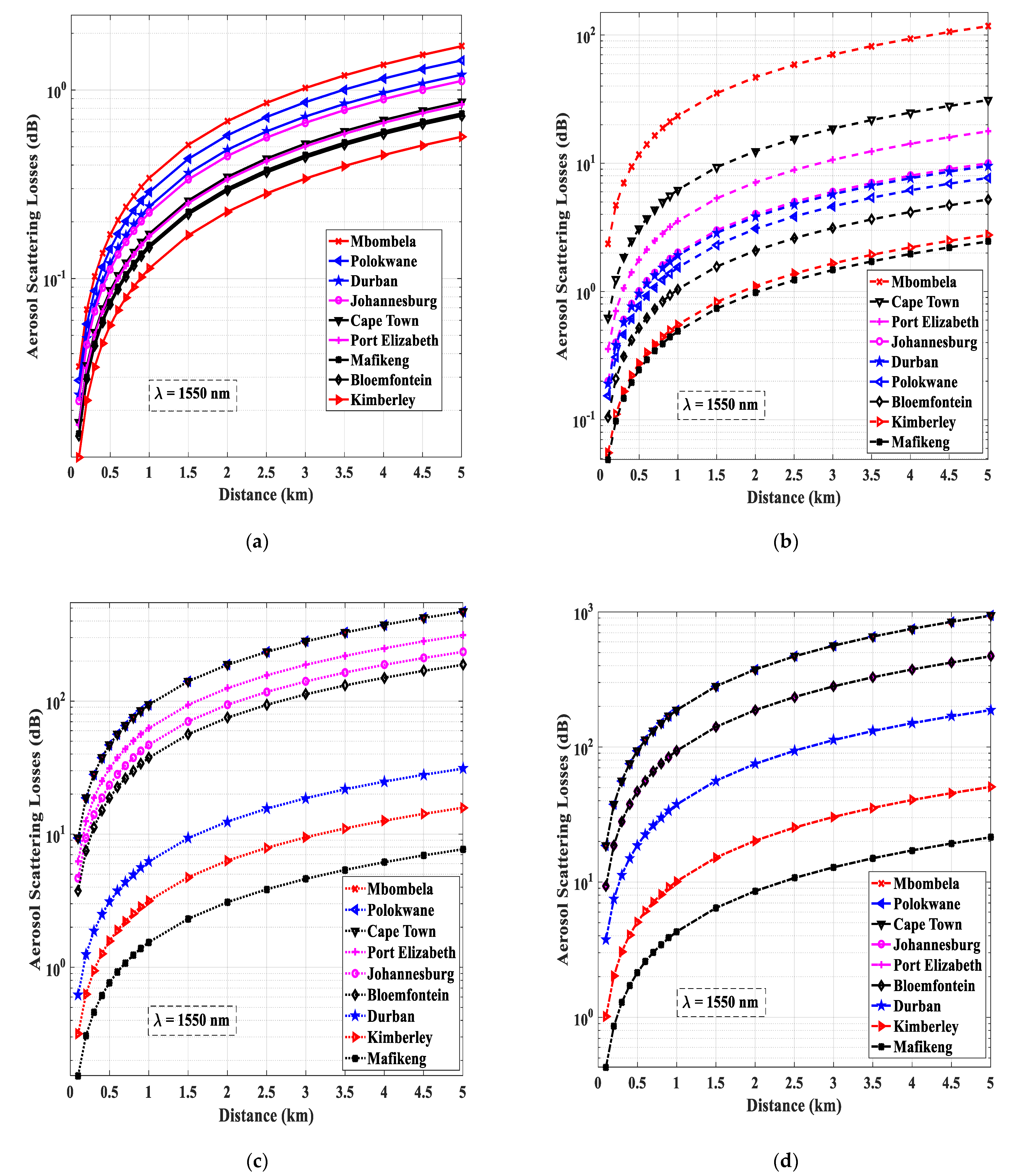
4. Aerosol Scattering Losses

The aerosol scattering coefficient in dB/km, as defined by the Kim and Ijaz models, is given in [42] as:

$${{\displaystyle L}}_{Sca}=\frac{17}{V}{{\displaystyle \left(\frac{\lambda }{{{\displaystyle \lambda }}_{\circ }}\right)}}^{-{{\displaystyle q}}_{\circ }}$$

(25)

where $V$ is the meteorological visibility in km, ${{\displaystyle \lambda }}_o=550 \mathrm{nm}$ is the maximum spectrum wavelength of the solar band, and ${{\displaystyle q}}_{\circ }$ is the particle size distribution parameter. In the Kim model, ${{\displaystyle q}}_{\circ }$ is expressed in terms of visibility as [48]:

$${{\displaystyle q}}_{\circ }\left(V\right)=\left\{\begin{array}{ccc}1.6& for& V>50 \mathrm{km}\\ 1.3& for& 6<V<50 \mathrm{km}\\ 0.16V+0.34& for& 1<V<6 \mathrm{km}\end{array}\right.$$

(26)

while ${{\displaystyle q}}_{\circ }$ is expressed in terms of wavelength in the Ijaz model as [49,50]:

$${{\displaystyle q}}_{\circ }\left(\lambda \right)=0.1428\lambda -0.0947$$

(27)

For visibility measurements less than 1 km, the Ijaz model is used to calculate scattering losses, while the Kim model is used to calculate the specific attenuation associated with visibility values greater than or equal to 1 km. The two models are used in estimating scattering losses encountered by the transmission wavelength of 1550 nm. The visibility data used in computing the aerosol scattering losses over different distances in Figure 4a–d was obtained from the SAWS for the nine major South African cities of interest investigated in this work. The data was collected three times daily (8:00 a.m., 2:00 p.m., and 8:00 p.m.) over an 8½ year period (January 2010 until June 2018). Over a link distance of 1 km, FSOC links transmitting at 1550 nm in Mbombela would encounter scattering losses of ~0.34, 23, 94, and 188 dB based on the periods not exceeded 50%, 99%, 99.9%, and 99.99% of the time, respectively.

Similarly, scattering losses of ~0.15, 0.50, 1.54, and 4.29 dB would be encountered by the same FSOC links over a distance of 1 km in the city of Mafikeng, as shown in Figure 4a–d, respectively.

5. Intensity Distribution

In this section, the statistical analysis of the irradiance fluctuations and the channel characteristics for the weak and moderate to strong turbulence regimes are carried out using the Lognormal and Gamma–gamma turbulence distributions, respectively. The PDF of the lognormal distribution is given in [14,15,17,18] as:

$${{\displaystyle f}}_I\left(I\right)=\frac{{{\displaystyle I}}^{-1}}{{{\displaystyle \sigma }}_{SI}\sqrt{2\pi }}\exp \left\{-{{\displaystyle \left(\frac{In\left(I\right)+\left(0.5{{\displaystyle \sigma }}_{SI}^2\right)}{{{\displaystyle \sigma }}_{SI}\sqrt{2}}\right)}}^2\right\}$$

(28)

While the PDF of the Gamma–gamma turbulence distribution can be expressed as [17,39,51,52]:

$${{\displaystyle f}}_I\left(I\right)=\frac{{{\displaystyle 2I}}^{-1}{{\displaystyle \left(\alpha \beta I\right)}}^{0.5\left(\alpha +\beta \right)}}{\mathsf{\Gamma }\left(\alpha \right)\mathsf{\Gamma }\left(\beta \right)}{{\displaystyle K}}_{\alpha -\beta }\left(2\sqrt{\alpha \beta I}\right)$$

(29)

where $I$ is the normalized irradiance, $\mathsf{\Gamma }\left(·\right)$ represents the Gamma function, and ${{\displaystyle K}}_{\alpha -\beta }\left(·\right)$ is the modified Bessel function of the second kind and of order $\alpha -\beta$. $\alpha$ is the effective number of large-scale turbulence eddies. It is defined as [43]:

$$\alpha ={{\displaystyle \left({{\displaystyle \sigma }}_x^2\right)}}^{-1}={{\displaystyle \left(\exp \left({{\displaystyle \sigma }}_{\ln x}^2\right)-1\right)}}^{-1}$$

(30)

where ${{\displaystyle \sigma }}_x^2$ is the normalized large-scale (refractive) variance. $\beta$ is the effective number of small-scale turbulence eddies. It is given as [43]:

$$\beta ={{\displaystyle \left({{\displaystyle \sigma }}_y^2\right)}}^{-1}={{\displaystyle \left(\exp \left({{\displaystyle \sigma }}_{\ln y}^2\right)-1\right)}}^{-1}$$

(31)

where ${{\displaystyle \sigma }}_y^2$ is the normalized small-scale (diffractive) variance. Using equation (07.34.03.0605.01) in [53], where:

$${{\displaystyle G}}_{0,2}^{2,0}\left[\alpha \beta I\left|\alpha ,\beta \right.\right]=2{{\displaystyle \left(\alpha \beta I\right)}}^{0.5\left(\alpha +\beta \right)}{{\displaystyle K}}_{\alpha -\beta }\left(2\sqrt{\alpha \beta I}\right)$$

(32)

Equation (29) can be rewritten as:

$${{\displaystyle f}}_I\left(I\right)=\frac{{{\displaystyle I}}^{-1}}{\mathsf{\Gamma }\left(\alpha \right)\mathsf{\Gamma }\left(\beta \right)}{{\displaystyle G}}_{0,2}^{2,0}\left[\alpha \beta I\left|\begin{array}{c}-\\ \alpha ,\beta \end{array}\right.\right],I>0$$

(33)

where ${{\displaystyle G}}_{u,v}^{s,t}\left(z\left|\begin{array}{c}{{\displaystyle a}}_1,\dots ,{{\displaystyle a}}_p\\ {{\displaystyle c}}_1,\dots ,{{\displaystyle c}}_p\end{array}\right.\right)$ is the Meijer G function, which is well defined in [54]. Integrating ${{\displaystyle f}}_I\left(I\right)$ in Equation (33) gives the CDF of $I$. This is derived by using equation (07.34.21.0003.01) in [53]. Thus, we have:

$${{\displaystyle F}}_I\left(I\right)=\frac{1}{\mathsf{\Gamma }\left(\alpha \right)\mathsf{\Gamma }\left(\beta \right)}{{\displaystyle G}}_{1,3}^{2,1}\left[\alpha \beta I\left|\begin{array}{c}1\\ \alpha ,\beta ,0\end{array}\right.\right],I>0$$

(34)

In this work, pointing errors represent the misalignment between the transmitter and receiver caused by the laser beam being displaced horizontally or vertically, i.e., a two-dimensional configuration is being considered. The transmitter and receiver planes are assumed to be parallel, and the laser beam is perpendicular to the receiver area. The pointing error parameter, $\xi$, is defined as the ratio between the equivalent beam waist or radius at the receiver (${{\displaystyle W}}_{Leq}$) and the standard deviation of the jitter or pointing error at the receiver (${{\displaystyle \sigma }}_s$). It can be expressed as [6,16,55,56]:

$$\xi =\frac{{{\displaystyle W}}_{Leq}}{2{{\displaystyle \sigma }}_s}$$

(35)

The beam waist ${{\displaystyle W}}_L$ of a Gaussian beam, which is the radius calculated at ${{\displaystyle e}}^2$, determines the value of the parameter, ${{\displaystyle W}}_{Leq}$ at distance, $L$. ${{\displaystyle W}}_{Leq}$ is given as [6,16,18,55,56,57]:

$${{\displaystyle W}}_{Leq}={{\displaystyle \left(\frac{{{\displaystyle W}}_L^2\sqrt{\pi }erf\left(v\right)}{2v\exp \left({{\displaystyle -v}}^2\right)}\right)}}^{0.5}$$

(36)

where ${{\displaystyle W}}_L={{\displaystyle {{\displaystyle W}}_o}}_{\sqrt{\left({{\displaystyle \mathsf{\Theta }}}_o+{{\displaystyle \mathsf{\Lambda }}}_o\right)\left(1+\left(1.63{{\displaystyle \mathsf{\Lambda }}}_1{{\displaystyle \sigma }}_1^{2.4}\right)\right)}}$, $erf\left(.\right)$ is the error function and parameter $v$ is expressed as [6,16,55,56]:

$$v=\frac{r\sqrt{\pi }}{{{\displaystyle W}}_L\sqrt{2}}$$

(37)

where $r$ represents the radius of a circular detector aperture. At distance $L=0$, the fraction of the collected power is represented by parameter ${{\displaystyle A}}_o$. It is expressed as [6,16,55,56]:

$${{\displaystyle A}}_o={{\displaystyle \left[erf\left(v\right)\right]}}^2={{\displaystyle \left[1-erfc\left(v\right)\right]}}^2$$

(38)

where $erfc\left(.\right)$ is the complementary error function.

Therefore, the PDF of the Lognormal distribution, considering the effect of pointing errors, is derived in [17,18,58] as:

$${{\displaystyle f}}_I\left(I\right)=\frac{{{\displaystyle \xi }}^2}{{{\displaystyle \left({{\displaystyle A}}_o\right)}}^{{{\displaystyle \xi }}^2}}{{\displaystyle I}}^{{{\displaystyle \xi }}^2-1}\frac{1}{2}\exp \left(q\right)erfc\left(\frac{In\left(\raisebox{1ex}{$I$}\!\left/ \!\raisebox{-1ex}{${{\displaystyle A}}_o$}\right.\right)+p}{{{\displaystyle \sigma }}_{SI}\sqrt{2}}\right)$$

(39)

where

$$p=0.5{{\displaystyle \sigma }}_{SI}^2+{{\displaystyle \xi }}^2{{\displaystyle \sigma }}_{SI}^2$$

(40)

and

$$q=\frac{{{\displaystyle \xi }}^2{{\displaystyle \sigma }}_{SI}^2\left(1+{{\displaystyle \xi }}^2\right)}{2}$$

(41)

Additionally, the PDF of the Gamma–gamma distribution model, taking into account the effects of misalignment, is derived in [6,16,56] as:

$${{\displaystyle f}}_I\left(I\right)=\frac{{{\displaystyle \alpha \beta \xi }}^2}{{{\displaystyle A}}_o\mathsf{\Gamma }\left(\alpha \right)\mathsf{\Gamma }\left(\beta \right)}{{\displaystyle G}}_{1,3}^{3,0}\left[\frac{\alpha \beta }{{{\displaystyle A}}_o}I\left|\begin{array}{c}{{\displaystyle \xi }}^2\\ {{\displaystyle \xi }}^2-1,\alpha -1,\beta -1\end{array}\right.\right],I>0$$

(42)

After some mathematical manipulations, the PDF can be further simplified as [6,56]:

$${{\displaystyle f}}_I\left(I\right)=\frac{{{\displaystyle I}}^{-1}{{\displaystyle \xi }}^2}{\mathsf{\Gamma }\left(\alpha \right)\mathsf{\Gamma }\left(\beta \right)}{{\displaystyle G}}_{1,3}^{3,0}\left[\frac{\alpha \beta {{\displaystyle \xi }}^2}{{{\displaystyle \xi }}^2+1}I\left|\begin{array}{c}{{\displaystyle \xi }}^2+1\\ {{\displaystyle \xi }}^2,\alpha ,\beta \end{array}\right.\right],I\ge 0$$

(43)

The expression for the CDF of the Gamma–gamma distribution model, considering pointing error effects, is derived in [6,56] as:

$${{\displaystyle F}}_I\left(I\right)=\frac{{{\displaystyle \xi }}^2}{\mathsf{\Gamma }\left(\alpha \right)\mathsf{\Gamma }\left(\beta \right)}{{\displaystyle G}}_{2,4}^{3,1}\left[\frac{\alpha \beta {{\displaystyle \xi }}^2}{{{\displaystyle \xi }}^2+1}I\left|\begin{array}{c}{{\displaystyle 1,\xi }}^2+1\\ {{\displaystyle \xi }}^2,\alpha ,\beta ,0\end{array}\right.\right]$$

(44)

For commercial FSOC links employing the use of intensity modulation/direct detection (IM/DD) schemes and avalanche photodiode (APD) detectors, the instantaneous signal-to-noise ratio (SNR) at the receiver is defined as [42,56,59,60]:

$$\gamma =\frac{{{\displaystyle \left(2\Re {{\displaystyle g}}_a{{\displaystyle P}}_{x}I\right)}}^2}{{{\displaystyle \sigma }}_n^2}=\overline{\gamma }{{\displaystyle I}}^2$$

(45)

where $\Re$ is the responsivity, ${{\displaystyle g}}_a$ is the APD gain, ${{\displaystyle \sigma }}_n^2$ is the total noise at the APD receiver, and ${{\displaystyle P}}_x$ is the average optical power detected at the receiver. ${{\displaystyle P}}_x$ is well defined in Equation (9) of [42].

The average SNR at the receiver is defined as [42,56]:

$$\overline{\gamma }=\frac{{{\displaystyle \left(2\Re {{\displaystyle g}}_a{{\displaystyle P}}_x\right)}}^2}{{{\displaystyle \sigma }}_n^2}$$

(46)

The total noise at the APD receiver comprises the thermal and shot noise. It is given as [42,51,59,60]:

$${{\displaystyle \sigma }}_n^2=\frac{4T{{\displaystyle K}}_b{{\displaystyle R}}_b{{\displaystyle F}}_n}{R}I+2q\Re {{\displaystyle g}}_a^2{{\displaystyle F}}_a{{\displaystyle R}}_b{{\displaystyle P}}_{x}I$$

(47)

where $T$ is the temperature of the receiver, ${{\displaystyle K}}_b$ is the Boltzmann constant, ${{\displaystyle R}}_b$ is the bit rate, ${{\displaystyle F}}_n$ is the noise figure of the amplifier, $R$ is the APD load resistance, $q$ is the electron charge, and ${{\displaystyle F}}_a$ is excess noise factor. The excess noise factor is expressed as [42,51,59,60]:

$${{\displaystyle F}}_a=2-{{\displaystyle g}}_a^{-1}-2{{\displaystyle k}}_a+{{\displaystyle k}}_a{{\displaystyle g}}_a^{-1}+{{\displaystyle k}}_a{{\displaystyle g}}_a$$

(48)

where ${{\displaystyle k}}_a$ is the ionization factor.

The PDF of SNRs for weak atmospheric turbulence using the Lognormal distribution model with pointing errors is derived by substituting Equation (45) into Equation (39), and is given below as [18]:

$${{\displaystyle f}}_{\gamma }\left(\gamma \right)=\frac{{{\displaystyle 0.5\xi }}^2}{{{\displaystyle \left({{\displaystyle A}}_o\right)}}^{{{\displaystyle \xi }}^2}}\frac{{{\displaystyle \gamma }}^{\left({{\displaystyle 0.5\xi }}^2\right)-1}}{{{\displaystyle \overline{\gamma }}}^{{{\displaystyle 0.5\xi }}^2}}\frac{1}{\sqrt{\pi }}\exp \left(q\right)erfc\left(\frac{0.5In\left(\frac{\gamma }{\overline{\gamma }{{\displaystyle A}}_o^2}\right)+p}{{{\displaystyle \sigma }}_{SI}\sqrt{2}}\right)$$

(49)

Applying the relation in [18,31] where:

$$Q\left(\gamma \right)=0.5erfc\left(\frac{\gamma }{\sqrt{2}}\right)\approx \frac{1}{12}\exp \left(-\frac{{{\displaystyle \gamma }}^2}{2}\right)+\frac{1}{4}\exp \left(-\frac{2{{\displaystyle \gamma }}^2}{3}\right)$$

(50)

Equation (49) becomes:

$${{\displaystyle f}}_{\gamma }\left(\gamma \right)=\frac{{{\displaystyle \xi }}^2}{{{\displaystyle \left({{\displaystyle A}}_o\right)}}^{{{\displaystyle \xi }}^2}}\frac{{{\displaystyle \gamma }}^{\left({{\displaystyle 0.5\xi }}^2\right)-1}}{{{\displaystyle \overline{\gamma }}}^{{{\displaystyle 0.5\xi }}^2}}\frac{1}{\sqrt{\pi }}\exp \left(q\right)\left[\frac{1}{12}\exp \left(-\frac{1}{2}{{\displaystyle \left(\frac{0.5In\left(\frac{\gamma }{\overline{\gamma }{{\displaystyle A}}_o^2}\right)+p}{{{\displaystyle \sigma }}_{SI}}\right)}}^2\right)+\frac{1}{4}\exp \left(-\frac{2}{3}{{\displaystyle \left(\frac{0.5In\left(\frac{\gamma }{\overline{\gamma }{{\displaystyle A}}_o^2}\right)+p}{{{\displaystyle \sigma }}_{SI}}\right)}}^2\right)\right]$$

(51)

The PDF of SNRs for moderate to strong atmospheric turbulence using the Gamma–gamma model with pointing errors, as derived in [55,56], is given as:

$${{\displaystyle f}}_{\gamma }\left(\gamma \right)=\frac{{{\displaystyle \gamma }}^{-1}{{\displaystyle \xi }}^2}{2\mathsf{\Gamma }\left(\alpha \right)\mathsf{\Gamma }\left(\beta \right)}{{\displaystyle G}}_{1,3}^{3,0}\left[\frac{\alpha \beta {{\displaystyle \xi }}^2}{{{\displaystyle \xi }}^2+1}{{\displaystyle \left(\frac{\gamma }{\overline{\gamma }}\right)}}^{0.5}\left|\begin{array}{c}{{\displaystyle \xi }}^2+1\\ {{\displaystyle \xi }}^2,\alpha ,\beta \end{array}\right.\right]$$

(52)

The ${{\displaystyle \sigma }}_{SI}^2\left(0,L\right)$ is used in characterizing the atmospheric turbulence strength due to the effect of scintillation. In a weak turbulence regime, ${{\displaystyle \sigma }}_{SI}^2\left(0,L\right)<1$, and the Lognormal distribution model is employed. For moderate to strong fluctuations, ${{\displaystyle \sigma }}_{SI}^2\left(0,L\right)\ge 1$, and the Gamma–gamma turbulence distribution is used [38,44]. In certain instances where ${{\displaystyle \sigma }}_{SI}^2\left(0,L\right)<1$ but $\alpha \beta \le 10$ or $\mathsf{\Gamma }\left(\alpha \right)\mathsf{\Gamma }\left(\beta \right)\le 50$, then the Gamma–gamma distribution is employed. In other situations, where ${{\displaystyle \sigma }}_{SI}^2\left(0,L\right)<1$ and $\mathsf{\Gamma }\left(\alpha \right)\mathsf{\Gamma }\left(\beta \right)\ge 100$ or $\alpha \beta \ge 20$, some computations involving the Gamma–gamma distribution would produce undefined results [43]. Thus, in this work, when ${{\displaystyle \sigma }}_{SI}^2\left(0,L\right)<1$ and $\alpha \beta >10$ or $\mathsf{\Gamma }\left(\alpha \right)\mathsf{\Gamma }\left(\beta \right)>50$, the Lognormal distribution is used.

6. Outage Probability Analysis

Outage probability is a critical performance indicator that defines the likelihood of the instantaneous SNR going below the threshold SNR. Once this occurs, the link’s communication will fail. It is expressed below as [45,61]:

$${{\displaystyle \mathrm{Pr}}}_{out}=\mathrm{Pr}obability\left[\gamma \le {{\displaystyle \gamma }}_{th}\right]={{\displaystyle F}}_{\gamma }\left[{{\displaystyle \gamma }}_{th}\right]$$

(53)

where ${{\displaystyle \gamma }}_{th}$ is the threshold SNR and ${{\displaystyle F}}_{\gamma }\left[{{\displaystyle \gamma }}_{th}\right]$ is the CDF of the instantaneous SNR.

From Equation (45), the normalized irradiance at the receiver can be expressed as [6,57]:

$$I={{\displaystyle \left(\frac{\gamma }{\overline{\gamma }}\right)}}^{0.5}={{\displaystyle \left(\frac{{{\displaystyle \gamma }}_{th}}{\overline{\gamma }}\right)}}^{0.5}$$

(54)

Therefore, substituting for $I$ in Equation (44) presents the expression for estimating the outage probability of the FSO link over the turbulent atmospheric channel while considering the effect of pointing errors [6,56]:

$${{\displaystyle \mathrm{Pr}}}_{out}=\frac{{{\displaystyle \xi }}^2}{\mathsf{\Gamma }\left(\alpha \right)\mathsf{\Gamma }\left(\beta \right)}{{\displaystyle G}}_{2,4}^{3,1}\left[\frac{\alpha \beta {{\displaystyle \xi }}^2}{{{\displaystyle \xi }}^2+1}{{\displaystyle \left(\frac{{{\displaystyle \gamma }}_{th}}{\overline{\gamma }}\right)}}^{0.5}\left|\begin{array}{c}{{\displaystyle 1,\xi }}^2+1\\ {{\displaystyle \xi }}^2,\alpha ,\beta ,0\end{array}\right.\right]$$

(55)

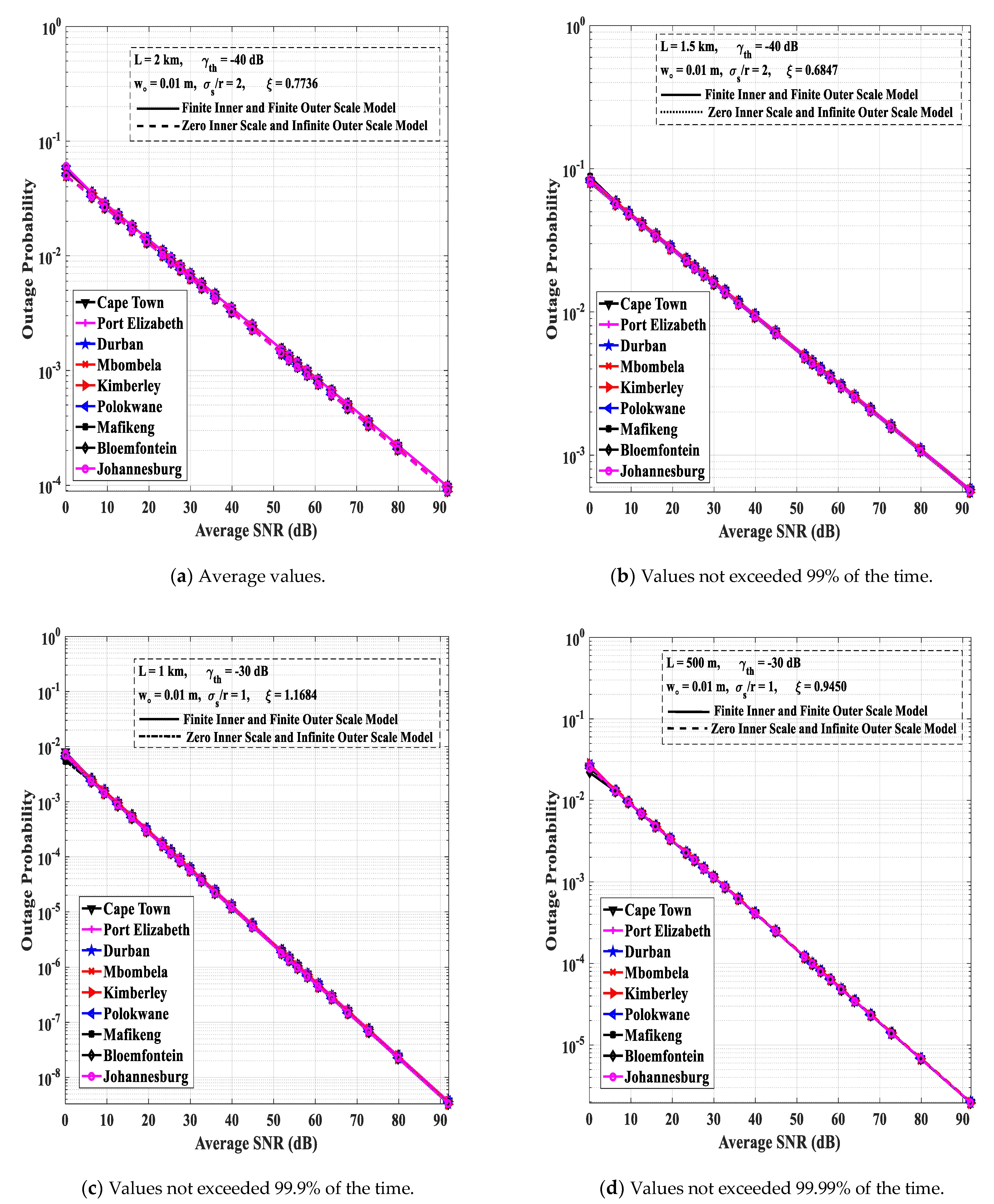
Figure 5a–d are based on the numerical values in Table 2, Table 3, Table 4 and Table 5, respectively. These figures are generated using the parameters in

Table 6. Commercial FSOC link parameters used in computations.

FSOC Link Parameters
Light Source	Laser
Wavelength $\left(\lambda \right)$	1550 nm
Transmit Power $\left({{\displaystyle P}}_T\right)$	20 dBm
Receiver Sensitivity $\left({{\displaystyle R}}_S\right)$	−40 dBm
Receiver Aperture Diameter $\left(D\right)$	10 cm
Eye Safety	Class 1M
Transmit Beam Divergence Angle $\left(\varphi \right)$	1.75 mrad
Responsivity $\left(\Re \right)$	0.5 A/W
Bit Rate $\left({{\displaystyle R}}_b\right)$	10 Gb/s
Detector	Avalanche Photodiode (APD)
Boltzmann’s Constant $\left({{\displaystyle K}}_b\right)$	1.381 × 10−23 J/K
Temperature $\left(T\right)$	298 K
Planck’s Constant $\left(h\right)$	6.626 × 10−34 Js
Speed of Light $\left(c\right)$	3 × 108 m/s
APD Load Resistance $\left(R\right)$	1000 Ω
APD Gain $\left({{\displaystyle g}}_a\right)$	50
Amplifier Noise Figure $\left({{\displaystyle F}}_n\right)$	2
Charge of an Electron	1.602 × 10−19 C
Ionization factor for InGaAs APD $\left({{\displaystyle k}}_a\right)$	0.7

, while computing with Equations (1)–(3), (15), (30), (31), (35), (46) and (55). The average receiver SNRs needed to achieve various outage probabilities over different link distances while considering the effect of pointing errors in the presence of turbulent eddies are presented in Figure 5a–d for the locations of interest. In these figures, the average receiver SNRs required to attain different outage probabilities are quite similar. It is also evident from these figures that the impact of the normalized jitter standard deviation on the outage probability is significant (when comparing Figure 5c,d where $\frac{{{\displaystyle \sigma }}_s}{r}=1$ to Figure 5a,b where $\frac{{{\displaystyle \sigma }}_s}{r}=2$). This implies that the lower the value of $\frac{{{\displaystyle \sigma }}_s}{r}$, the better the overall system performance. Additionally, the higher the value of $\xi$, the better the outage probability performance of the FSOC links. In the presence of finite inner and outer scales of turbulence, that is, where l_o = 0.005 m and L_o = 10 m, the outage probabilities of the FSOC links are quite similar to when these turbulent eddies have sizes of zero and infinity in the Kolmogorov model with an infinitely large inertial range.

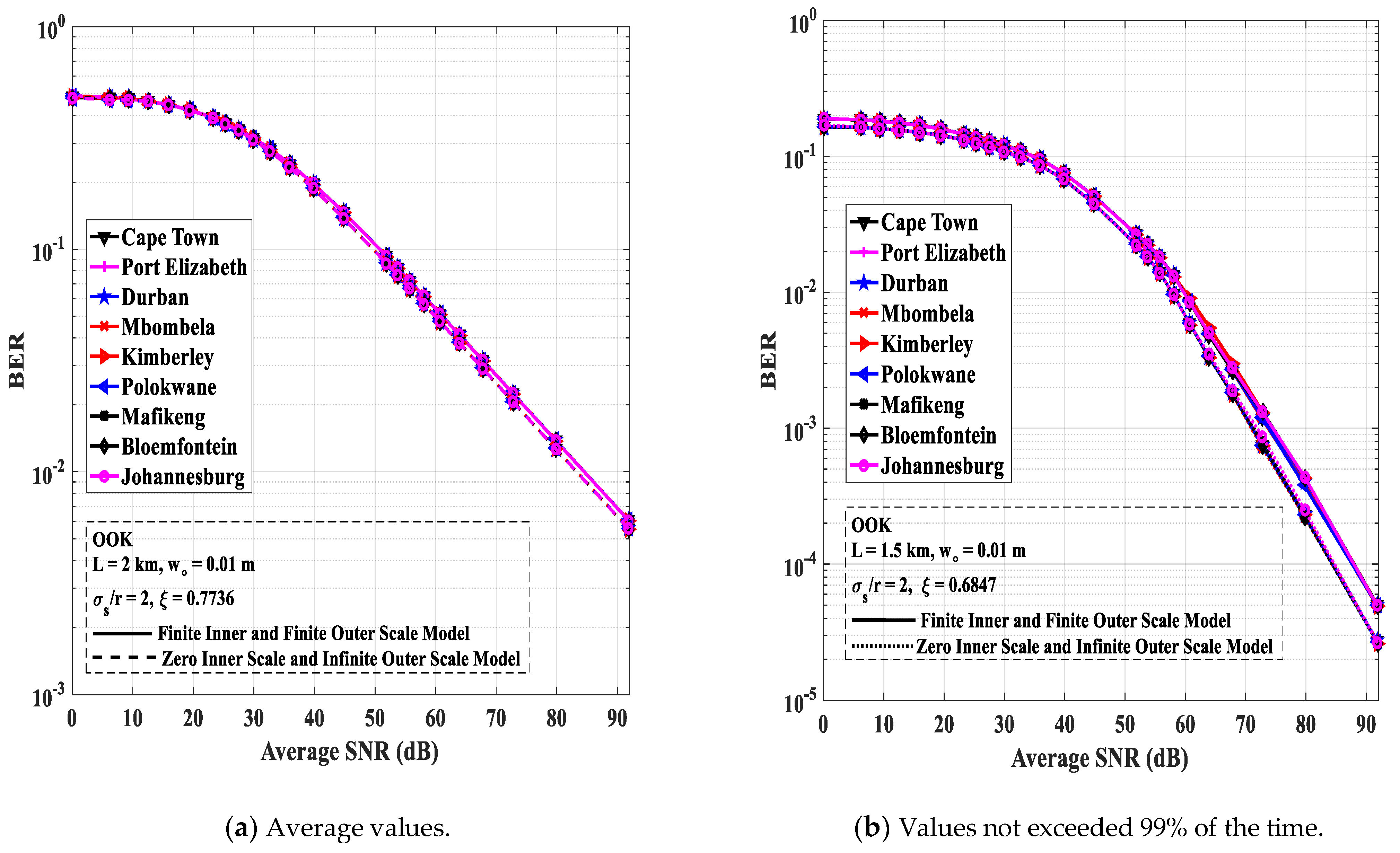
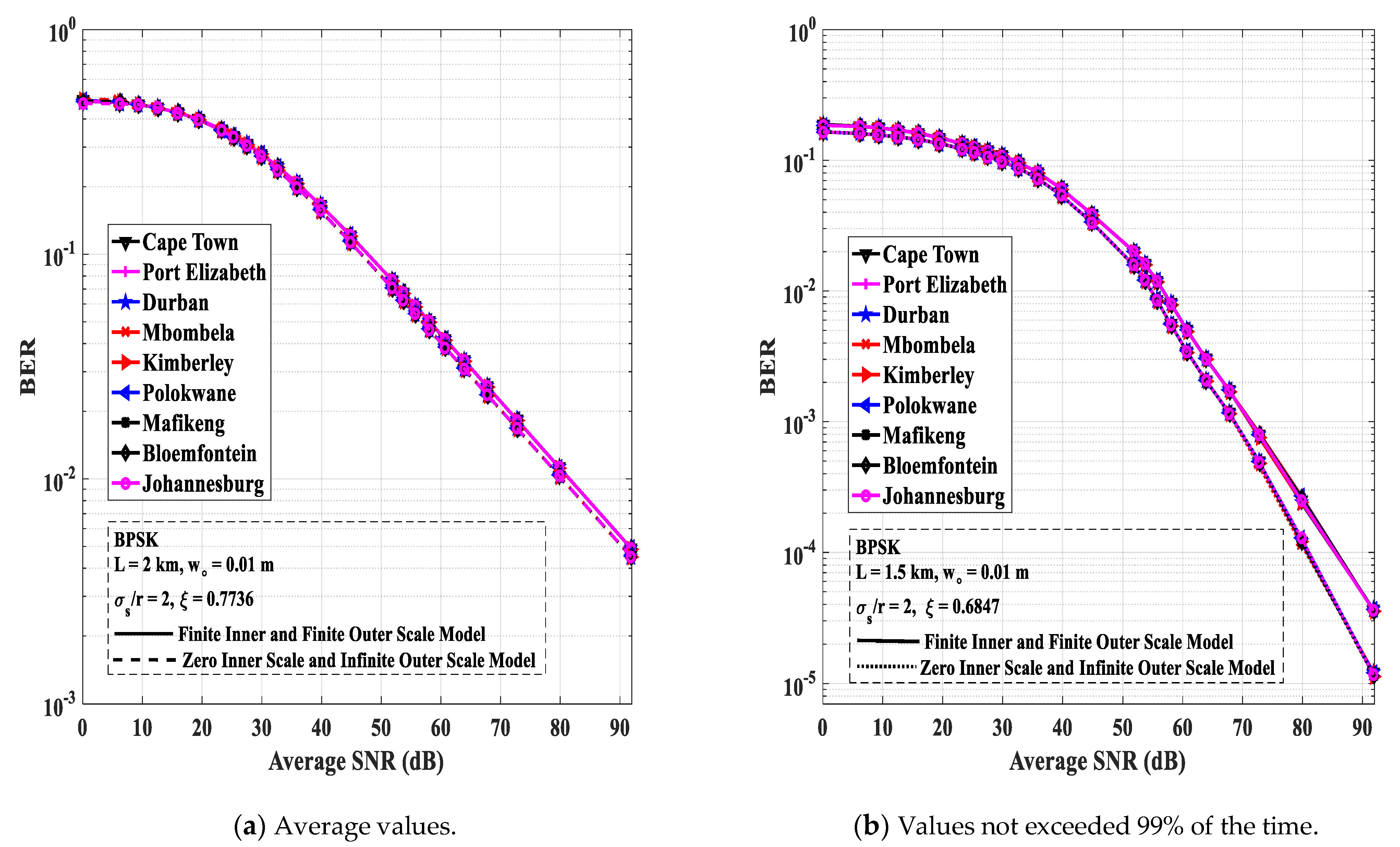
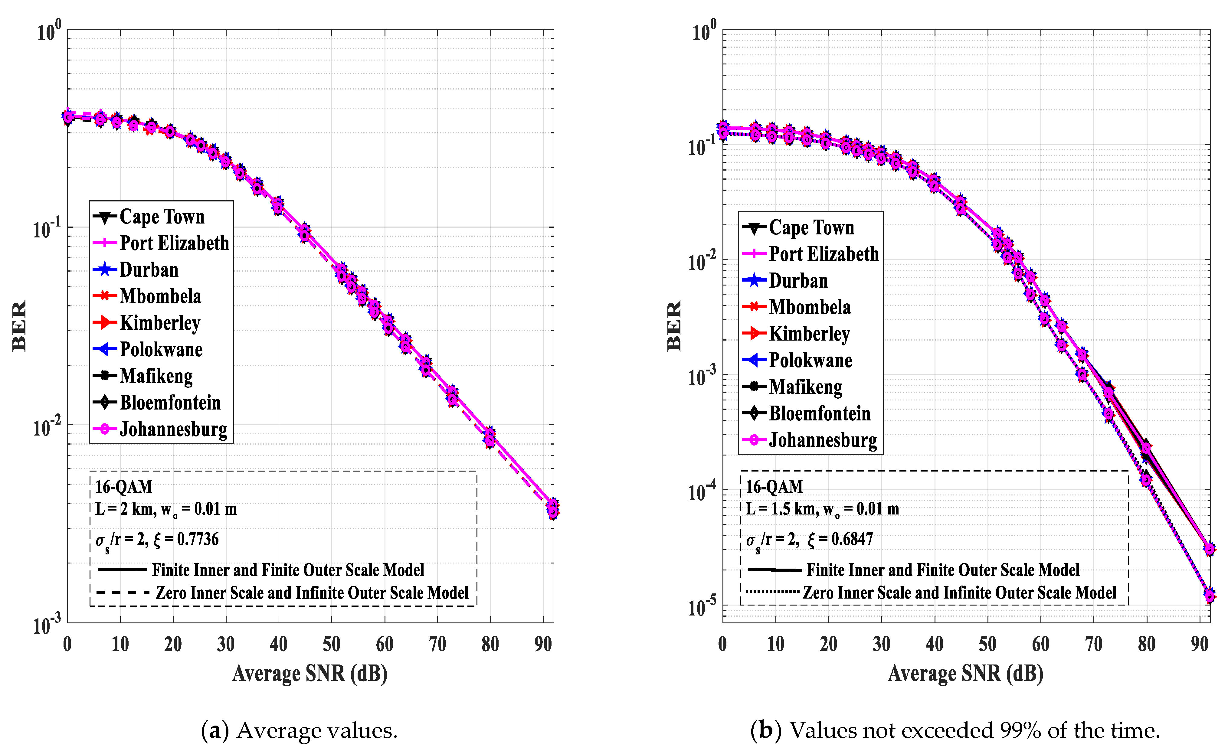
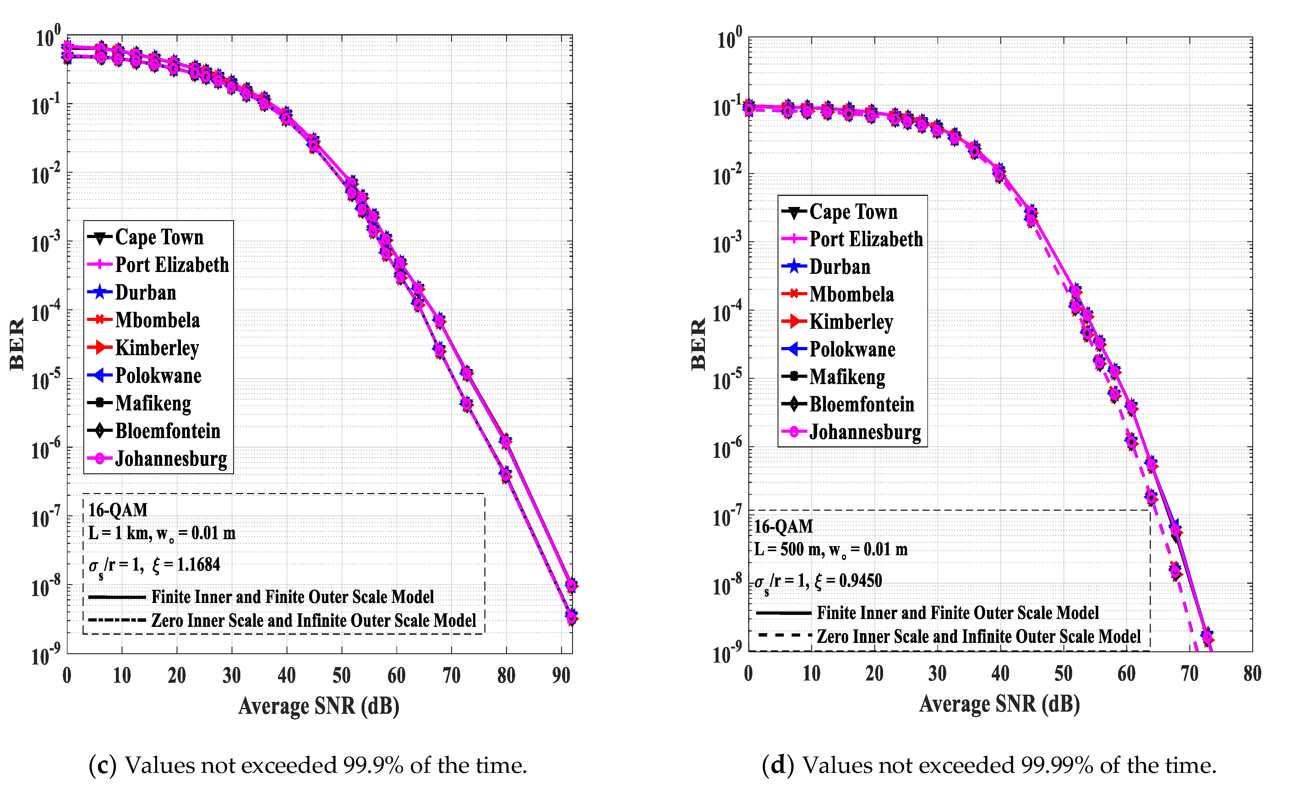
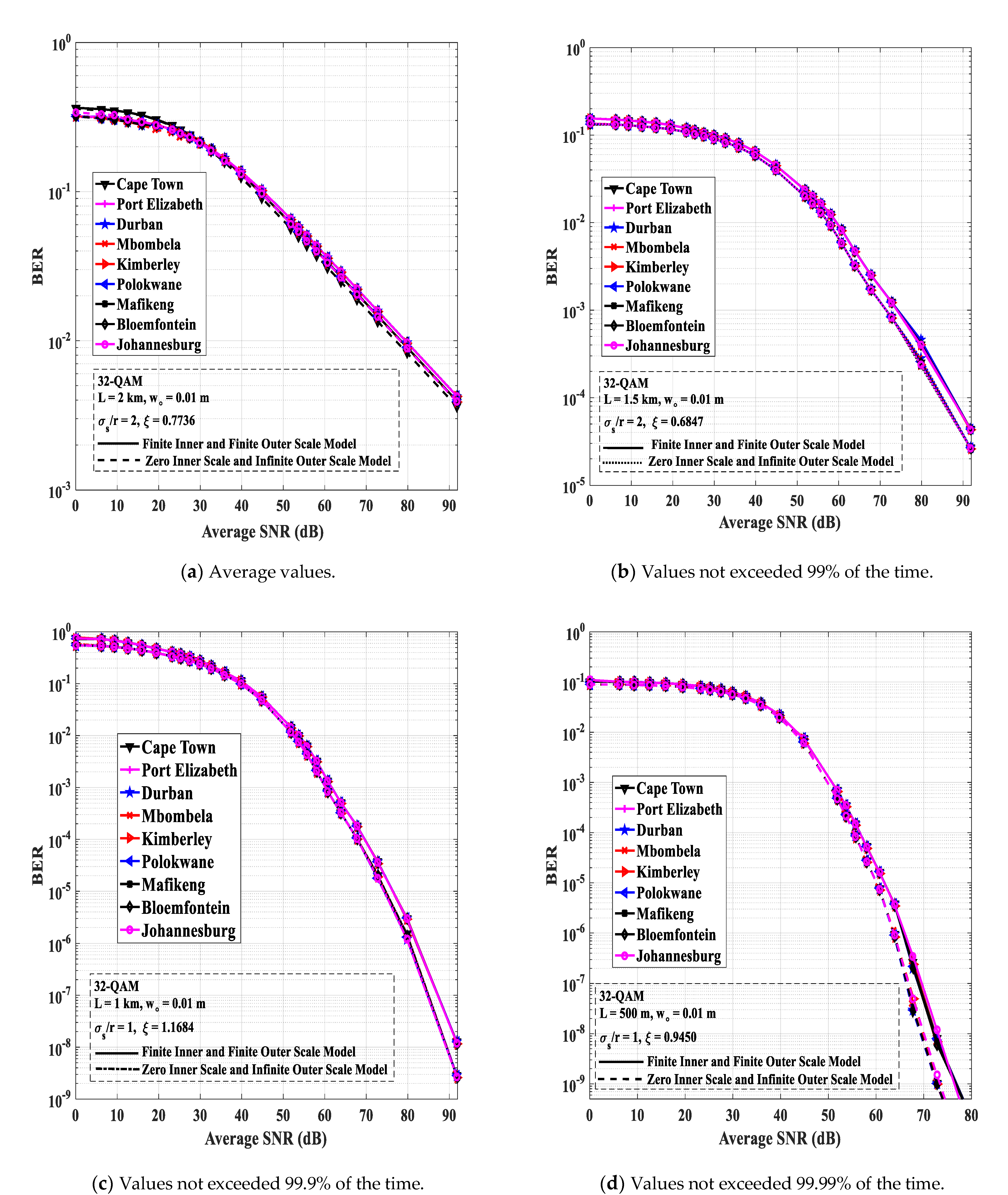
7. Average Bit Error Rate (BER) Analysis

The average BER of an IM/DD single-input single-output (SISO) FSOC link based on a specific modulation scheme during periods of atmospheric turbulence is defined as [31,56,58]:

$${{\displaystyle P}}_{BER}={\displaystyle \underset{0}{\overset{\infty }{\int }}P\left(e|\gamma \right)}{{\displaystyle f}}_{\gamma }\left(\gamma \right)d\gamma$$

(56)

where $P\left(e|\gamma \right)$ is the conditional BER of the FSO link based on a specific modulation scheme and ${{\displaystyle f}}_{\gamma }\left(\gamma \right)$ represent the PDFs of the Lognormal and Gamma–gamma turbulence models while considering the effects of pointing errors in Equations (51) and (52), respectively.

7.1. Return-to-Zero On-Off Keying (RZ-OOK) FSOC Links

The conditional BER for RZ-OOK SISO FSOC links in the absence of atmospheric turbulence is given as [56]:

$${{\displaystyle P}}_{RZ-OOK}\left(e/\gamma \right)=Q\left(\frac{\sqrt{2\gamma }}{2}\right)=0.5erfc\left(0.5{{\displaystyle \gamma }}^{0.5}\right)$$

(57)

• Weak Atmospheric Turbulence

In order to derive the expression for the BER of RZ-OOK SISO FSOC links in the presence of weak atmospheric turbulence, inserting Equations (51) and (57) into Equation (56) yields:

$${{\displaystyle P}}_{RZ-OOK}={\displaystyle \underset{0}{\overset{\infty }{\int }}\left(0.5erfc\left(0.5{{\displaystyle \gamma }}^{0.5}\right)•\frac{{{\displaystyle \xi }}^2}{{{\displaystyle \left({{\displaystyle A}}_o\right)}}^{{{\displaystyle \xi }}^2}}\frac{{{\displaystyle \gamma }}^{\left({{\displaystyle 0.5\xi }}^2\right)-1}}{{{\displaystyle \overline{\gamma }}}^{{{\displaystyle 0.5\xi }}^2}}\frac{\exp \left(q\right)}{\sqrt{\pi }}•\left[\frac{1}{12}\exp \left(-{{\displaystyle \left(\frac{0.5In\left(\frac{\gamma }{\overline{\gamma }{{\displaystyle A}}_o^2}\right)+p}{{{\displaystyle 4\sigma }}_{SI}}\right)}}^2\right)+\frac{1}{4}\exp \left(-{{\displaystyle \left(\frac{2In\left(\frac{\gamma }{\overline{\gamma }{{\displaystyle A}}_o^2}\right)+4p}{{{\displaystyle 9\sigma }}_{SI}}\right)}}^2\right)\right]\right)d\gamma }$$

(58)

Variable substitutions where:

$${{\displaystyle z}}_1=\frac{0.5In\left(\frac{\gamma }{\overline{\gamma }{{\displaystyle A}}_o^2}\right)+p}{{{\displaystyle 4\sigma }}_{SI}}$$

(59)

and

$${{\displaystyle z}}_2=\frac{2In\left(\frac{\gamma }{\overline{\gamma }{{\displaystyle A}}_o^2}\right)+4p}{{{\displaystyle 9\sigma }}_{SI}}$$

(60)

are employed. Making $\gamma$ the subject of (59) and (60) yields:

$$\gamma ={{\displaystyle \overline{\gamma }A}}_o^2\exp \left(8{{\displaystyle z}}_1{{\displaystyle \sigma }}_{SI}-2p\right)$$

(61)

and

$$\gamma ={{\displaystyle \overline{\gamma }A}}_o^2\exp \left(4.5{{\displaystyle z}}_2{{\displaystyle \sigma }}_{SI}-2p\right)$$

(62)

Differentiating $\gamma$ with respect to ${{\displaystyle z}}_1$ and ${{\displaystyle z}}_2$ in (61) and (62), respectively, gives:

$$d\gamma =8{{\displaystyle \overline{\gamma }A}}_o^2{{\displaystyle \sigma }}_{SI}\exp \left(8{{\displaystyle z}}_1{{\displaystyle \sigma }}_{SI}-2p\right)d{{\displaystyle z}}_1$$

(63)

and

$$d\gamma =4.5{{\displaystyle \overline{\gamma }A}}_o^2{{\displaystyle \sigma }}_{SI}\exp \left(4.5{{\displaystyle z}}_2{{\displaystyle \sigma }}_{SI}-2p\right)d{{\displaystyle z}}_2$$

(64)

Therefore, substituting Equations (59)–(63) and (64) in Equation (58) generates:

$$\begin{array}{c}{{\displaystyle P}}_{RZ-OOK}={\displaystyle \underset{0}{\overset{\infty }{\int }}\left(\frac{{{\displaystyle {{\displaystyle \xi }}^2\sigma }}_{SI}\exp (q)}{3\sqrt{\pi }}\left({{\displaystyle \left(\exp \left({{\displaystyle 8z}}_1{{\displaystyle \sigma }}_{SI}-2p\right)\right)}}^{\left({{\displaystyle 0.5\xi }}^2\right)}•erfc\left(\frac{\sqrt{{{\displaystyle \overline{\gamma }A}}_o^2\exp \left({{\displaystyle 8z}}_1{{\displaystyle \sigma }}_{SI}-2p\right)}}{2}\right)\right)•\exp \left(-{{\displaystyle z}}_1^2\right)\right)d{{\displaystyle z}}_1}\\ +\\ {\displaystyle \underset{0}{\overset{\infty }{\int }}\left(\frac{{{\displaystyle {{\displaystyle 9\xi }}^2\sigma }}_{SI}\exp (q)}{16\sqrt{\pi }}\left({{\displaystyle \left(\exp \left({{\displaystyle 4.5z}}_2{{\displaystyle \sigma }}_{SI}-2p\right)\right)}}^{\left({{\displaystyle 0.5\xi }}^2\right)}•erfc\left(\frac{\sqrt{{{\displaystyle \overline{\gamma }A}}_o^2\exp \left({{\displaystyle 4.5z}}_2{{\displaystyle \sigma }}_{SI}-2p\right)}}{2}\right)\right)•\exp \left(-{{\displaystyle z}}_2^2\right)\right)d{{\displaystyle z}}_2}\end{array}$$

(65)

Since a closed form solution does not exist for the above integration, the Gauss–Hermite quadrature approximation, as presented in [62,63], is used to evaluate the integration, where:

$${\displaystyle \underset{-\infty }{\overset{\infty }{\int }}\exp \left(-{{\displaystyle x}}^2\right)}f\left(x\right)dx\cong {\displaystyle \sum _{i=1}^N{{\displaystyle W}}_i}f\left({{\displaystyle z}}_i\right)$$

(66)

Therefore, the BER of RZ-OOK SISO FSOC links in the presence of weak atmospheric turbulence and pointing errors is:

$${{\displaystyle P}}_{RZ-OOK}=\frac{{{\displaystyle {{\displaystyle \xi }}^2\sigma }}_{SI}\exp (q)}{2\sqrt{\pi }}•\left(\begin{array}{c}\left(\frac{1}{3}{\displaystyle \sum _{i=1}^N{{\displaystyle W}}_i\left({{\displaystyle \left(\exp \left({{\displaystyle 8z}}_1{{\displaystyle \sigma }}_{SI}-2p\right)\right)}}^{\left({{\displaystyle 0.5\xi }}^2\right)}•erfc\left(\frac{\sqrt{{{\displaystyle \overline{\gamma }A}}_o^2\exp \left({{\displaystyle 8z}}_1{{\displaystyle \sigma }}_{SI}-2p\right)}}{2}\right)\right)}\right)\\ +\\ \left(\frac{9}{16}{\displaystyle \sum _{i=1}^N{{\displaystyle W}}_i\left({{\displaystyle \left(\exp \left({{\displaystyle 4.5z}}_2{{\displaystyle \sigma }}_{SI}-2p\right)\right)}}^{\left({{\displaystyle 0.5\xi }}^2\right)}•erfc\left(\frac{\sqrt{{{\displaystyle \overline{\gamma }A}}_o^2\exp \left({{\displaystyle 4.5z}}_2{{\displaystyle \sigma }}_{SI}-2p\right)}}{2}\right)\right)}\right)\end{array}\right)$$

(67)

where the values of the weights, ${{\displaystyle W}}_i$, and zeros of the Hermite polynomial, ${{\displaystyle z}}_i$, are given in [62,63].

2.

Moderate to Strong Atmospheric Turbulence

Applying equation (07.34.03.0619.01) in [53] to Equation (57), we obtain:

$${{\displaystyle G}}_{1,2}^{2,0}\left[0.25\gamma \left|\begin{array}{c}1\\ 0,0.5\end{array}\right.\right]={{\displaystyle \pi }}^{0.5}erfc\left(0.5{{\displaystyle \gamma }}^{0.5}\right)$$

(68)

Therefore, combining Equations (57) and (68) yields:

$${{\displaystyle P}}_{RZ-OOK}(e|\gamma )=\frac{0.5}{{{\displaystyle \pi }}^{0.5}}{{\displaystyle G}}_{1,2}^{2,0}\left[0.25\gamma \left|\begin{array}{c}1\\ 0,0.5\end{array}\right.\right]$$

(69)

Inserting Equations (52) and (69) into Equation (56) gives:

$${{\displaystyle P}}_{RZ-OOK}=\frac{{{\displaystyle \xi }}^2}{4\mathsf{\Gamma }\left(\alpha \right)\mathsf{\Gamma }\left(\beta \right){{\displaystyle \pi }}^{0.5}}•{\displaystyle \underset{0}{\overset{\infty }{\int }}{{\displaystyle {{\displaystyle \gamma }}^{-1}•G}}_{1,2}^{2,0}\left[0.25\gamma \left|\begin{array}{c}1\\ 0,0.5\end{array}\right.\right]•}{{\displaystyle G}}_{1,3}^{3,0}\left[\frac{\alpha \beta {{\displaystyle \xi }}^2}{{{\displaystyle \xi }}^2+1}{{\displaystyle \left(\frac{\gamma }{\overline{\gamma }}\right)}}^{0.5}\left|\begin{array}{c}{{\displaystyle \xi }}^2+1\\ {{\displaystyle \xi }}^2,\alpha ,\beta \end{array}\right.\right]d\gamma$$

(70)

Applying equation (07.34.21.0013.01) in [53] to evaluate Equation (70) yields:

$${{\displaystyle P}}_{RZ-OOK}=\frac{{{\displaystyle {{\displaystyle \xi }}^{2}2}}^{\alpha +\beta -4}}{{{\displaystyle \pi }}^{1.5}\mathsf{\Gamma }\left(\alpha \right)\mathsf{\Gamma }\left(\beta \right)}{{\displaystyle G}}_{4,7}^{6,2}\left[{{\displaystyle \left(\frac{\alpha \beta {{\displaystyle \xi }}^2}{{{\displaystyle \xi }}^2+1}\right)}}^2\frac{1}{4\overline{\gamma }}\left|\begin{array}{c}1,0.5,\frac{{{\displaystyle \xi }}^2+1}{2},\frac{{{\displaystyle \xi }}^2+2}{2}\\ \frac{{{\displaystyle \xi }}^2}{2},\frac{{{\displaystyle \xi }}^2+1}{2},\frac{\alpha }{2},\frac{\alpha +1}{2},\frac{\beta }{2},\frac{\beta +1}{2},0\end{array}\right.\right]$$

(71)

Further simplification of Equation (71) gives:

$${{\displaystyle P}}_{RZ-OOK}=\frac{{{\displaystyle {{\displaystyle \xi }}^{2}2}}^{\alpha +\beta -4}}{{{\displaystyle \pi }}^{1.5}\mathsf{\Gamma }\left(\alpha \right)\mathsf{\Gamma }\left(\beta \right)}{{\displaystyle G}}_{3,6}^{5,2}\left[{{\displaystyle \left(\frac{\alpha \beta {{\displaystyle \xi }}^2}{{{\displaystyle \xi }}^2+1}\right)}}^2\frac{1}{4\overline{\gamma }}\left|\begin{array}{c}1,0.5,\frac{{{\displaystyle \xi }}^2+2}{2}\\ \frac{{{\displaystyle \xi }}^2}{2},\frac{\alpha }{2},\frac{\alpha +1}{2},\frac{\beta }{2},\frac{\beta +1}{2},0\end{array}\right.\right]$$

(72)

In Figure 6b–d, the BER results of the FSOC links in all the cities of interest are generated using Equations (1)–(3), (15), (35), (38), (40), (41), (46) and (67) because the scintillation parameters in those locations fall within the weak atmospheric turbulence regime over a link distance of 1.5, 1, and 0.5 km, respectively. The BER results of the cities in Figure 6a are computed using Equations (1)–(3), (15), (30), (31), (35) (46) and (72). Figure 6a–d present the BERs computed for the zero inner scale and infinite outer scale model and finite inner and finite outer scale model for different receive SNRs, and are based on the numerical values in Table 2, Table 3, Table 4, and Table 5, respectively.

It is imperative to state that the presence of misalignment errors ($\frac{{{\displaystyle \sigma }}_s}{r}=2$) in Figure 6a,b strongly impacts on the BER performance of the FSOC links, while the low presence of pointing errors ($\frac{{{\displaystyle \sigma }}_s}{r}=1$) in Figure 6c,d indicate better BERs for all the locations investigated. Additionally, the presence of the inner and outer scales of turbulence where l_o = 0.005 m and L_o = 10 m, cause poorer BERs when compared to the results of the zero inner scale and infinite outer scale model. It is also important to note that the inner scale bump is responsible for the higher values of scintillation obtained when the modified atmospheric spectrum is employed. The BER performances of the FSOC links deployed in the cities investigated are quite similar, as shown in the four figures.

7.2. Binary Phase Shift Keying (BPSK) FSOC Links

The conditional BER for BPSK SISO FSOC links in the absence of atmospheric turbulence is presented in [57,64] as:

$${{\displaystyle P}}_{BPSK}\left(e/\gamma \right)=Q\left(\sqrt{\gamma }\right)=0.5erfc\left(\frac{{{\displaystyle \gamma }}^{0.5}}{\sqrt{2}}\right)$$

(73)

• Weak Atmospheric Turbulence

Inserting Equations (51) and (73) into Equation (56) yields the expression for the BER of BPSK SISO FSOC links in the presence of weak atmospheric turbulence and pointing errors:

$${{\displaystyle P}}_{BPSK}={\displaystyle \underset{0}{\overset{\infty }{\int }}\left(0.5erfc\left(\frac{{{\displaystyle \gamma }}^{0.5}}{\sqrt{2}}\right)•\frac{{{\displaystyle \xi }}^2}{{{\displaystyle \left({{\displaystyle A}}_o\right)}}^{{{\displaystyle \xi }}^2}}\frac{{{\displaystyle \gamma }}^{\left({{\displaystyle 0.5\xi }}^2\right)-1}}{{{\displaystyle \overline{\gamma }}}^{{{\displaystyle 0.5\xi }}^2}}\frac{\exp \left(q\right)}{\sqrt{\pi }}•\left[\frac{1}{12}\exp \left(-{{\displaystyle \left(\frac{0.5In\left(\frac{\gamma }{\overline{\gamma }{{\displaystyle A}}_o^2}\right)+p}{{{\displaystyle 4\sigma }}_{SI}}\right)}}^2\right)+\frac{1}{4}\exp \left(-{{\displaystyle \left(\frac{2In\left(\frac{\gamma }{\overline{\gamma }{{\displaystyle A}}_o^2}\right)+4p}{{{\displaystyle 9\sigma }}_{SI}}\right)}}^2\right)\right]\right)d\gamma }$$

(74)

Further simplification of Equation (74), by substituting Equations (59)–(63) and (64) into it, gives an expression in the form:

$$\begin{array}{c}{{\displaystyle P}}_{BPSK}={\displaystyle \underset{0}{\overset{\infty }{\int }}\left(\frac{{{\displaystyle {{\displaystyle \xi }}^2\sigma }}_{SI}\exp (q)}{3\sqrt{\pi }}\left({{\displaystyle \left(\exp \left({{\displaystyle 8z}}_1{{\displaystyle \sigma }}_{SI}-2p\right)\right)}}^{\left({{\displaystyle 0.5\xi }}^2\right)}•erfc\left(\frac{\sqrt{{{\displaystyle \overline{\gamma }A}}_o^2\exp \left({{\displaystyle 8z}}_1{{\displaystyle \sigma }}_{SI}-2p\right)}}{\sqrt{2}}\right)\right)•\exp \left(-{{\displaystyle z}}_1^2\right)\right)d{{\displaystyle z}}_1}\\ +\\ {\displaystyle \underset{0}{\overset{\infty }{\int }}\left(\frac{{{\displaystyle {{\displaystyle 9\xi }}^2\sigma }}_{SI}\exp (q)}{16\sqrt{\pi }}\left({{\displaystyle \left(\exp \left({{\displaystyle 4.5z}}_2{{\displaystyle \sigma }}_{SI}-2p\right)\right)}}^{\left({{\displaystyle 0.5\xi }}^2\right)}•erfc\left(\frac{\sqrt{{{\displaystyle \overline{\gamma }A}}_o^2\exp \left({{\displaystyle 4.5z}}_2{{\displaystyle \sigma }}_{SI}-2p\right)}}{\sqrt{2}}\right)\right)•\exp \left(-{{\displaystyle z}}_2^2\right)\right)d{{\displaystyle z}}_2}\end{array}$$

(75)

Therefore, evaluating Equation (75) using the Gauss–Hermite quadrature approximation in Equation (66) yields the BER of BPSK SISO FSOC links in the presence of weak atmospheric turbulence and pointing errors:

$${{\displaystyle P}}_{BPSK}=\frac{{{\displaystyle {{\displaystyle \xi }}^2\sigma }}_{SI}\exp (q)}{2\sqrt{\pi }}•\left(\begin{array}{c}\left(\frac{1}{3}{\displaystyle \sum _{i=1}^N{{\displaystyle W}}_i\left({{\displaystyle \left(\exp \left({{\displaystyle 8z}}_1{{\displaystyle \sigma }}_{SI}-2p\right)\right)}}^{\left({{\displaystyle 0.5\xi }}^2\right)}•erfc\left(\frac{\sqrt{{{\displaystyle \overline{\gamma }A}}_o^2\exp \left({{\displaystyle 8z}}_1{{\displaystyle \sigma }}_{SI}-2p\right)}}{\sqrt{2}}\right)\right)}\right)\\ +\\ \left(\frac{9}{16}{\displaystyle \sum _{i=1}^N{{\displaystyle W}}_i\left({{\displaystyle \left(\exp \left({{\displaystyle 4.5z}}_2{{\displaystyle \sigma }}_{SI}-2p\right)\right)}}^{\left({{\displaystyle 0.5\xi }}^2\right)}•erfc\left(\frac{\sqrt{{{\displaystyle \overline{\gamma }A}}_o^2\exp \left({{\displaystyle 4.5z}}_2{{\displaystyle \sigma }}_{SI}-2p\right)}}{\sqrt{2}}\right)\right)}\right)\end{array}\right)$$

(76)

where the values of the weights, ${{\displaystyle W}}_i$, and zeros of the Hermite polynomial, ${{\displaystyle z}}_i$, are given in [62,63].

2.

Moderate to Strong Atmospheric Turbulence

The conditional BER for BPSK SISO FSOC links in terms of the Meijer G function and in the absence of atmospheric turbulence is presented in [65] as:

$${{\displaystyle P}}_{BPSK}(e|\gamma )=\frac{0.5}{{{\displaystyle \pi }}^{0.5}}{{\displaystyle G}}_{1,2}^{2,0}\left[0.5\gamma \left|\begin{array}{c}1\\ 0,0.5\end{array}\right.\right]$$

(77)

Substituting Equations (52) and (77) into Equation (56) gives:

$${{\displaystyle P}}_{BPSK}=\frac{{{\displaystyle \xi }}^2}{4\mathsf{\Gamma }\left(\alpha \right)\mathsf{\Gamma }\left(\beta \right){{\displaystyle \pi }}^{0.5}}•{\displaystyle \underset{0}{\overset{\infty }{\int }}{{\displaystyle {{\displaystyle \gamma }}^{-1}•G}}_{1,2}^{2,0}\left[0.5\gamma \left|\begin{array}{c}1\\ 0,0.5\end{array}\right.\right]•}{{\displaystyle G}}_{1,3}^{3,0}\left[\frac{\alpha \beta {{\displaystyle \xi }}^2}{{{\displaystyle \xi }}^2+1}{{\displaystyle \left(\frac{\gamma }{\overline{\gamma }}\right)}}^{0.5}\left|\begin{array}{c}{{\displaystyle \xi }}^2+1\\ {{\displaystyle \xi }}^2,\alpha ,\beta \end{array}\right.\right]d\gamma$$

(78)

Applying equation (07.34.21.0013.01) in [53] to evaluate Equation (78) yields:

$${{\displaystyle P}}_{BPSK}=\frac{{{\displaystyle {{\displaystyle \xi }}^{2}2}}^{\alpha +\beta -4}}{{{\displaystyle \pi }}^{1.5}\mathsf{\Gamma }\left(\alpha \right)\mathsf{\Gamma }\left(\beta \right)}{{\displaystyle G}}_{4,7}^{6,2}\left[{{\displaystyle \left(\frac{\alpha \beta {{\displaystyle \xi }}^2}{{{\displaystyle \xi }}^2+1}\right)}}^2\frac{1}{8\overline{\gamma }}\left|\begin{array}{c}1,0.5,\frac{{{\displaystyle \xi }}^2+1}{2},\frac{{{\displaystyle \xi }}^2+2}{2}\\ \frac{{{\displaystyle \xi }}^2}{2},\frac{{{\displaystyle \xi }}^2+1}{2},\frac{\alpha }{2},\frac{\alpha +1}{2},\frac{\beta }{2},\frac{\beta +1}{2},0\end{array}\right.\right]$$

(79)

The BERs estimated for the zero inner scale and infinite outer scale model and finite inner and finite outer scale model for different receive SNRs are presented in Figure 7a–d, and are based on the numerical values in Table 2, Table 3, Table 4 and Table 5, respectively.

Equations (1)–(3), (15), (35), (38), (40), (41), (46) and (76) are employed for plotting the BER results of the FSOC links deployed in all the cities in Figure 7b–d, while Figure 7a is computed using Equations (1)–(3), (15), (30), (31), (35), (46) and (79). Figure 7a–d also show that the presence of finite microscale and macroscale eddies result in poorer BER performances when compared with instances when those eddies have sizes of zero and infinity in the Kolmogorov model with infinitely large inertial range. In order to obtain a BER of 10⁻² over a link distance of 2 km for FSOC links in all the cities investigated, receive SNRs of ~84 and ~81 dB are required based on the finite inner and finite outer scale model in Figure 6a and Figure 7a, respectively. The BPSK FSOC links investigated in Figure 7a–d generally outperform the OOK FSOC links in Figure 6a–d.

7.3. Quadrature Amplitude Modulation (SIM-QAM) FSOC Links

7.3.1. M-ary Square SIM-QAM FSOC Links

The conditional probability of error for M-ary square SIM-QAM signals in the absence of atmospheric turbulence as derived in [64,66] is given as:

$${{\displaystyle P}}_{MQAM}\left(e/\gamma \right)=\left(\frac{\sqrt{M}-1}{\sqrt{M}{{\displaystyle \log }}_2\sqrt{M}}\right)erfc\left(\sqrt{\frac{3{{\displaystyle \gamma \log }}_{2}M}{2\left(M-1\right)}}\right)$$

(80)

where $M$ is the even number of bits per symbol for square constellations.

• Weak Atmospheric Turbulence

Similar to the previous computations of the BER expressions of RZ-OOK and BPSK modulated signals, substituting Equations (53), (59)–(64) and (80) into Equation (56) gives:

$$\begin{array}{l}{{\displaystyle P}}_{MQAM}=\left(\frac{{{\displaystyle {{\displaystyle 2\xi }}^2\sigma }}_{SI}\exp (q)}{\sqrt{\pi }}•\frac{\sqrt{M}-1}{\sqrt{M}{{\displaystyle \log }}_2\sqrt{M}}\right)\times \\ \left(\begin{array}{c}{\displaystyle \underset{0}{\overset{\infty }{\int }}\left(\frac{1}{3}\left({{\displaystyle \left(\exp \left({{\displaystyle 8z}}_1{{\displaystyle \sigma }}_{SI}-2p\right)\right)}}^{\left({{\displaystyle 0.5\xi }}^2\right)}•erfc\left(\sqrt{\frac{{{\displaystyle 3{{\displaystyle \log }}_2\left(M\right)•\overline{\gamma }A}}_o^2\exp \left({{\displaystyle 8z}}_1{{\displaystyle \sigma }}_{SI}-2p\right)}{2\left(M-1\right)}}\right)\right)•\exp \left(-{{\displaystyle z}}_1^2\right)\right)d{{\displaystyle z}}_1}\\ +\\ {\displaystyle \underset{0}{\overset{\infty }{\int }}\left(\frac{9}{16}\left({{\displaystyle \left(\exp \left({{\displaystyle 4.5z}}_2{{\displaystyle \sigma }}_{SI}-2p\right)\right)}}^{\left({{\displaystyle 0.5\xi }}^2\right)}•erfc\left(\sqrt{\frac{{{\displaystyle 3{{\displaystyle \log }}_2\left(M\right)•\overline{\gamma }A}}_o^2\exp \left({{\displaystyle 4.5z}}_1{{\displaystyle \sigma }}_{SI}-2p\right)}{2\left(M-1\right)}}\right)\right)•\exp \left(-{{\displaystyle z}}_2^2\right)\right)d{{\displaystyle z}}_2}\end{array}\right)\end{array}$$

(81)

where further similar mathematical calculations produce the expression for the BER of M-ary square SIM-QAM SISO FSOC links in the presence of weak atmospheric turbulence and pointing errors:

$$\begin{array}{l}{{\displaystyle P}}_{MQAM}=\left(\frac{{{\displaystyle {{\displaystyle \xi }}^2\sigma }}_{SI}\exp (q)}{\sqrt{\pi }}•\frac{\sqrt{M}-1}{\sqrt{M}{{\displaystyle \log }}_2\sqrt{M}}\right)\times \\ \left(\begin{array}{c}\left(\frac{1}{3}{\displaystyle \sum _{i=1}^N{{\displaystyle W}}_i\left({{\displaystyle \left(\exp \left({{\displaystyle 8z}}_1{{\displaystyle \sigma }}_{SI}-2p\right)\right)}}^{\left({{\displaystyle 0.5\xi }}^2\right)}•erfc\left(\sqrt{\frac{{{\displaystyle 3{{\displaystyle \log }}_2\left(M\right)•\overline{\gamma }A}}_o^2\exp \left({{\displaystyle 8z}}_1{{\displaystyle \sigma }}_{SI}-2p\right)}{2\left(M-1\right)}}\right)\right)}\right)\\ +\\ \left(\frac{9}{16}{\displaystyle \sum _{i=1}^N{{\displaystyle W}}_i\left({{\displaystyle \left(\exp \left({{\displaystyle 4.5z}}_2{{\displaystyle \sigma }}_{SI}-2p\right)\right)}}^{\left({{\displaystyle 0.5\xi }}^2\right)}•erfc\left(\sqrt{\frac{{{\displaystyle 3{{\displaystyle \log }}_2\left(M\right)•\overline{\gamma }A}}_o^2\exp \left({{\displaystyle 4.5z}}_1{{\displaystyle \sigma }}_{SI}-2p\right)}{2\left(M-1\right)}}\right)\right)}\right)\end{array}\right)\end{array}$$

(82)

2.

Moderate to Strong Atmospheric Turbulence

The average BER for M-ary Square SIM-QAM SISO FSOC links in the presence of moderate to strong atmospheric turbulence, while taking in account the effect of pointing errors, is derived in [67] as:

$${{\displaystyle P}}_{MQAM}=\frac{{{\displaystyle {{\displaystyle \xi }}^{2}2}}^{\alpha +\beta -3}}{{{\displaystyle \pi }}^{1.5}\mathsf{\Gamma }\left(\alpha \right)\mathsf{\Gamma }\left(\beta \right)}\left(\frac{\sqrt{M}-1}{\sqrt{M}{{\displaystyle \log }}_2\sqrt{M}}\right){{\displaystyle G}}_{3,6}^{5,2}\left[{{\displaystyle \left(\frac{\alpha \beta {{\displaystyle \xi }}^2}{{{\displaystyle \xi }}^2+1}\right)}}^2\frac{\left(M-1\right)}{24\overline{\gamma }{{\displaystyle \log }}_{2}M}\left|\begin{array}{c}1,0.5,\frac{{{\displaystyle \xi }}^2+2}{2}\\ \frac{{{\displaystyle \xi }}^2}{2},\frac{\alpha }{2},\frac{\alpha +1}{2},\frac{\beta }{2},\frac{\beta +1}{2},0\end{array}\right.\right]$$

(83)

Equations (1)–(3), (15), (35), (38), (40), (41), (46) and (82) are used in plotting the BER results for the FSOC links in all the investigated cities based on the zero inner scale and infinite outer scale model and finite inner and finite outer scale model for different receive SNRs in Figure 8b–d. The results in Figure 8a are generated using Equations (1)–(3), (15), (30), (31), (35), (46) and (83). Additionally, the numerical values in Table 2, Table 3, Table 4 and Table 5 determine the BERs for the SIM 16-QAM FSOC links in Figure 8a–d. In the instance when turbulence eddies have sizes of zero and infinity in the Kolmogorov model with infinitely large inertial range, receive SNRs of ~70 dB are required to obtain a BER of 10⁻⁵ for 16-QAM FSOC links deployed in all the investigated cities, over a link distance of 1 km, as shown in Figure 8c.

The BERs of 16-QAM FSOC links in Figure 8a–d surpass the BER results of conventional OOK FSOC links in Figure 6a–d.

7.3.2. I × J Rectangular QAM FSOC Links

The conditional probability of error for I × J rectangular SIM-QAM signals in the absence of atmospheric turbulence is given in [66] as:

$${{\displaystyle P}}_{\left(I\times J\right)QAM}\left(e/\gamma \right)=\frac{1}{{{\displaystyle \log }}_2\left(I•J\right)}\left(\frac{I-1}{I}erfc\left(\sqrt{\frac{3{{\displaystyle \gamma \log }}_2\left(I•J\right)}{{{\displaystyle I}}^2+{{\displaystyle J}}^2-2}}\right)+\frac{J-1}{J}erfc\left(\sqrt{\frac{3{{\displaystyle \gamma \log }}_2\left(I•J\right)}{{{\displaystyle I}}^2+{{\displaystyle J}}^2-2}}\right)\right)$$

(84)

where $I$ and $J$ are the dimensions of the in-phase and quadrature signals [24,66].

• Weak Atmospheric Turbulence

Similarly, inserting Equations (53), (59)–(63), (64) and (84) into Equation (56) gives:

$$\begin{array}{l}{{\displaystyle P}}_{\left(I\times J\right)QAM}=\frac{{{\displaystyle {{\displaystyle 2\xi }}^2\sigma }}_{SI}\exp (q)}{\sqrt{\pi }{{\displaystyle \log }}_2\left(I•J\right)}•\left(\left(\frac{I-1}{I}\right)+\left(\frac{J-1}{J}\right)\right)\times \\ \left(\begin{array}{c}{\displaystyle \underset{0}{\overset{\infty }{\int }}\left(\frac{1}{3}\left({{\displaystyle \left(\exp \left({{\displaystyle 8z}}_1{{\displaystyle \sigma }}_{SI}-2p\right)\right)}}^{\left({{\displaystyle 0.5\xi }}^2\right)}•erfc\left(\sqrt{\frac{{{\displaystyle 3\overline{\gamma }A}}_o^2\exp \left({{\displaystyle 8z}}_1{{\displaystyle \sigma }}_{SI}-2p\right)•{{\displaystyle \log }}_2\left(I•J\right)}{{{\displaystyle I}}^2+{{\displaystyle J}}^2-2}}\right)\right)•\exp \left(-{{\displaystyle z}}_1^2\right)\right)d{{\displaystyle z}}_1}\\ +\\ {\displaystyle \underset{0}{\overset{\infty }{\int }}\left(\frac{9}{16}\left({{\displaystyle \left(\exp \left({{\displaystyle 4.5z}}_2{{\displaystyle \sigma }}_{SI}-2p\right)\right)}}^{\left({{\displaystyle 0.5\xi }}^2\right)}•erfc\left(\sqrt{\frac{{{\displaystyle 3\overline{\gamma }A}}_o^2\exp \left({{\displaystyle 4.5z}}_1{{\displaystyle \sigma }}_{SI}-2p\right)•{{\displaystyle \log }}_2\left(I•J\right)}{{{\displaystyle I}}^2+{{\displaystyle J}}^2-2}}\right)\right)•\exp \left(-{{\displaystyle z}}_2^2\right)\right)d{{\displaystyle z}}_2}\end{array}\right)\end{array}$$

(85)

Employing the Gauss–Hermite quadrature approximation in Equation (66) to evaluate Equation (85) generates the expression for the BER of I × J rectangular SIM-QAM SISO FSOC links in the presence of weak atmospheric turbulence and pointing errors:

$$\begin{array}{l}{{\displaystyle P}}_{\left(I\times J\right)QAM}=\frac{{{\displaystyle {{\displaystyle 2\xi }}^2\sigma }}_{SI}\exp (q)}{\sqrt{\pi }{{\displaystyle \log }}_2\left(I•J\right)}•\left(\left(\frac{I-1}{I}\right)+\left(\frac{J-1}{J}\right)\right)\times \\ \left(\begin{array}{c}\left(\frac{1}{3}{\displaystyle \sum _{i=1}^N{{\displaystyle W}}_i\left({{\displaystyle \left(\exp \left({{\displaystyle 8z}}_1{{\displaystyle \sigma }}_{SI}-2p\right)\right)}}^{\left({{\displaystyle 0.5\xi }}^2\right)}•erfc\left(\sqrt{\frac{{{\displaystyle 3\overline{\gamma }A}}_o^2\exp \left({{\displaystyle 8z}}_1{{\displaystyle \sigma }}_{SI}-2p\right)•{{\displaystyle \log }}_2\left(I•J\right)}{{{\displaystyle I}}^2+{{\displaystyle J}}^2-2}}\right)\right)}\right)\\ +\\ \left(\frac{9}{16}{\displaystyle \sum _{i=1}^N{{\displaystyle W}}_i\left({{\displaystyle \left(\exp \left({{\displaystyle 4.5z}}_2{{\displaystyle \sigma }}_{SI}-2p\right)\right)}}^{\left({{\displaystyle 0.5\xi }}^2\right)}•erfc\left(\sqrt{\frac{{{\displaystyle 3\overline{\gamma }A}}_o^2\exp \left({{\displaystyle 4.5z}}_1{{\displaystyle \sigma }}_{SI}-2p\right)•{{\displaystyle \log }}_2\left(I•J\right)}{{{\displaystyle I}}^2+{{\displaystyle J}}^2-2}}\right)\right)}\right)\end{array}\right)\end{array}$$

(86)

2.

Moderate to Strong Atmospheric Turbulence

The average BER for I × J Rectangular SIM-QAM SISO FSOC links in the presence of moderate to strong atmospheric turbulence while considering the effect pointing errors is presented in [67] as:

$${{\displaystyle P}}_{\left(I\times J\right)QAM}=\frac{{{\displaystyle {{\displaystyle \xi }}^{2}2}}^{\alpha +\beta -3}}{{{\displaystyle \pi }}^{1.5}\mathsf{\Gamma }\left(\alpha \right)\mathsf{\Gamma }\left(\beta \right)}\frac{1}{{{\displaystyle \log }}_2\left(I•J\right)}\left(\frac{I-1}{I}+\frac{J-1}{J}\right){{\displaystyle G}}_{3,6}^{5,2}\left[{{\displaystyle \left(\frac{\alpha \beta {{\displaystyle \xi }}^2}{{{\displaystyle \xi }}^2+1}\right)}}^2\frac{\left({{\displaystyle I}}^2+{{\displaystyle J}}^2-2\right)}{48\overline{\gamma }{{\displaystyle \log }}_2\left(I•J\right)}\left|\begin{array}{c}1,0.5,\frac{{{\displaystyle \xi }}^2+2}{2}\\ \frac{{{\displaystyle \xi }}^2}{2},\frac{\alpha }{2},\frac{\alpha +1}{2},\frac{\beta }{2},\frac{\beta +1}{2},0\end{array}\right.\right]$$

(87)

The BER performance of SIM rectangular 8 × 4 or 32-QAM FSOC links is presented for zero inner scale and infinite outer scale model and finite inner and finite outer scale model for different receive SNRs in Figure 9a–d.

In Figure 9b–d, the BER results of the FSOC links deployed in all the investigated cities are plotted using Equations (1)–(3), (15), (35), (38), (40), (41), (46) and (86), while the BER results in Figure 9a are computed using Equations (1)–(3), (15), (30), (31), (35), (46) and (87). Similarly, the results in Figure 9a–d are based on the numerical values in Table 2, Table 3, Table 4 and Table 5, respectively. As expected, the BER performance of SIM 32-QAM FSOC links is poorer than SIM 16-QAM FSOC links in Figure 8a–d, but the 32-QAM links transmits a greater amount of information. Additionally, when turbulence eddies have sizes of zero and infinity in the Kolmogorov model with an infinitely large inertial range, the BERs have better performances based on the zero inner scale and infinite outer scale model, as shown in Figure 9a–d.

8. Conclusions

In this paper, analysis of atmospheric turbulence effects on terrestrial SISO FSOC links based on the RMS and ground wind speeds prevalent in various cities of South Africa are presented. Wind speed data provided by the SAWS were statistically processed, and the corresponding CDF, PDF, and percentage of time plots are shown for each location of interest. The ${{\displaystyle C}}_n^2$ based on RMS wind speeds during clear and sunny weather are computed. The scintillation indices not exceeded 50%, 99%, 99.9%, and 99.99% of the time, based on the zero inner scale and infinite outer scale model and finite inner and finite outer scale model are calculated. Aerosol scattering losses based on visibilities not exceeded 50%, 99%, 99.9%, and 99.99% of the time for the various cities of South Africa are shown. Outage probability and BER analysis, taking into account the effect of pointing errors over weak and moderate to strong atmospheric turbulence channels, were then carried out for OOK, BPSK, and SIM-QAM SISO FSOC links deployed at the different locations of interest. All through Figure 5, Figure 6, Figure 7, Figure 8 and Figure 9, the SISO FSOC links deployed in all the locations of interest have similar outage probability and BER performances based on the zero inner scale and infinite outer scale model and finite inner and finite outer scale model. This is because the values of ${{\displaystyle C}}_n^2$ in all the investigated cities are approximately equivalent over all the time intervals (Table 2, Table 3, Table 4 and Table 5) considered in this work. As part of future work, all the analytical results in this work would be verified experimentally. The ${{\displaystyle C}}_n^2$ based on important meteorological parameters such as temperature, pressure, and the structure parameter for temperature, as well as three-dimensional pointing errors effects, will also be investigated for FSOC links deployed in the locations of interest.

References

1. ITU-R. Detailed Specifications of the Terrestrial Radio Interfaces of International Mobile Telecommunications-2020 (IMT-2020); Rec. ITU-R M.2150-0; M Series; ITU: Geneva, Switzerland, 2022; pp. 1–253. [Google Scholar]
2. Erunkulu, O.O.; Zungeru, A.M.; Lebekwe, C.K.; Mosalaosi, M.; Chuma, J.M. 5G mobile communication applications: A survey and comparison of use cases. IEEE Access 2021, 9, 97251–97295. [Google Scholar] [CrossRef]
3. Rasheed, I.; Hu, F. Intelligent super-fast Vehicle-to-Everything 5G communications with predictive switching between mmWave and THz links. Veh. Commun. 2021, 27, 100303. [Google Scholar] [CrossRef]
4. Lin, Y.B.; Tseng, C.C.; Wang, M.H. Effects of transport network slicing on 5G applications. Future Internet 2021, 13, 69. [Google Scholar] [CrossRef]
5. Siriwardhana, Y.; Porambage, P.; Liyanage, M.; Ylianttila, M. A Survey on Mobile Augmented Reality with 5G Mobile Edge Computing: Architectures, Applications, and Technical Aspects. IEEE Commun. Surv. Tutor. 2021, 23, 1160–1192. [Google Scholar] [CrossRef]
6. Malik, S.; Sahu, P.K. Free space optics/millimeter-wave based vertical and horizontal terrestrial backhaul network for 5G. Opt. Commun. 2020, 459, 125010. [Google Scholar] [CrossRef]
7. Palliyembil, V.; Vellakudiyan, J.; Muthuchidambaranathan, P. Performance analysis of RF-FSO communication systems over the Málaga distribution channel with pointing error. Optik 2021, 247, 167891. [Google Scholar] [CrossRef]
8. Garlinska, M.; Pregowska, A.; Masztalerz, K.; Osial, M. From mirrors to free-space optical communication—historical aspects in data transmission. Future Internet 2020, 12, 179. [Google Scholar] [CrossRef]
9. Kolawole, O.; Afullo, T.; Mosalaosi, M. Estimation of Optical Wireless Communication Link Availability Using Meteorological Visibility Data for Major Locations in South Africa. In Proceedings of the 2019 PhotonIcs & Electromagnetics Research Symposium-Spring (PIERS-Spring), Rome, Italy, 17–20 June 2019; pp. 319–325. [Google Scholar]
10. Kolawole, O.O.; Afullo, T.J.O.; Mosalaosi, M. Initial Modeling of Atmospheric Turbulence Effect on Optical Wireless Communication Links in South Africa. In Proceedings of the Southern Africa Telecommunication Networks and Applications Conference (SATNAC) 2019, Ballito, KwaZulu-Natal, South Africa, 1–4 September 2019; pp. 68–72. [Google Scholar]
11. Kolawole, O.O.; Afullo, T.J.O.; Owolawi, P.A. Performance Analysis of Cross M-QAM over Weak Atmospheric Turbulence Channel. In Proceedings of the Southern Africa Telecommunication Networks and Applications Conference (SATNAC) 2016, George, Western Cape, South Africa, 4–7 September 2016; pp. 80–84. [Google Scholar]
12. Dordová, L.; Wilfert, O. Calculation and comparison of turbulence attenuation by different methods. Radioengineering 2010, 19, 162–167. [Google Scholar]
13. Dubey, D.; Prajapati, Y.K.; Tripathi, R. Error performance analysis of PPM-and FSK-based hybrid modulation scheme for FSO satellite downlink. Opt. Quant. Elect. 2020, 52, 286. [Google Scholar]
14. AlQuwaiee, H.; Yang, H.; Alouini, M. On the Asymptotic Capacity of Dual-Aperture FSO Systems with Generalized Pointing Error Model. IEEE Trans. Wirel. Commun. 2016, 15, 6502–6512. [Google Scholar] [CrossRef] [Green Version]
15. Borah, D.K.; Voelz, D.G. Pointing Error Effects on Free-Space Optical Communication Links in the Presence of Atmospheric Turbulence. J. Lightwave Tech. 2009, 27, 3965–3973. [Google Scholar] [CrossRef]
16. Dubey, D.; Prajapati, Y.K.; Tripathi, R. Optimization of hybrid high-throughput MIMO system with misaligned FSO link under varied weather. Opt. Eng. 2021, 60, 086106. [Google Scholar] [CrossRef]
17. Farid, A.A.; Hranilovic, S. Outage Capacity Optimization for Free-Space Optical Links with Pointing Errors. J. Lightwave Tech. 2007, 25, 1702–1710. [Google Scholar] [CrossRef] [Green Version]
18. Trung, H.D.; Tuan, D.T.; Pham, A.T. Pointing error effects on performance of free-space optical communication systems using SC-QAM signals over atmospheric turbulence channels. AEU-Int. J. Electron. Commun. 2014, 68, 869–876. [Google Scholar] [CrossRef]
19. Ruiz, R.B.; Zambrana, A.G.; Vazquez, B.C.; Vazquez, C.C. Impact of nonzero boresight pointing error on ergodic capacity of MIMO FSO communication systems. Opt. Express 2016, 24, 3513–3534. [Google Scholar] [CrossRef] [PubMed]
20. Liu, H.; Liao, R.; Wei, Z.; Hou, Z.; Qiao, Y. BER analysis of a hybrid modulation scheme based on PPM and MSK subcarrier intensity modulation. IEEE Photonics J. 2015, 7, 7201510. [Google Scholar] [CrossRef]
21. Sharma, K.; Grewal, S.K. Performance assessment of hybrid PPM–BPSK–SIM based FSO communication system using time and wavelength diversity under variant atmospheric turbulence. Opt. Quant. Elect. 2020, 52, 430. [Google Scholar] [CrossRef]
22. Singya, P.K.; Shaik, P.; Kumar, N.; Bhatia, V.; Alouini, M.S. A Survey on Higher-Order QAM Constellations: Technical Challenges, Recent Advances, and Future Trends. IEEE Open J. Commun. Soc. 2021, 2, 617–655. [Google Scholar] [CrossRef]
23. Vu, B.T.; Truong, C.T.; Pham, A.T.; Dang, N.T. Performance of rectangular QAM/FSO systems using APD receiver over atmospheric turbulence channels. In Proceedings of the TENCON 2012 IEEE Region 10 Conference, Cebu, Philippines, 19–22 November 2012; pp. 1–5. [Google Scholar]
24. Vu, B.T.; Dang, N.T.; Thang, T.C.; Pham, A.T. Bit error rate analysis of rectangular QAM/FSO systems using an APD receiver over atmospheric turbulence channels. J. Opt. Commun. Netw. 2013, 5, 437–446. [Google Scholar] [CrossRef] [Green Version]
25. Sprung, D.; van Eijk, A.M.J.; Sucher, E.; Eisele, C.; Seiffer, D.; Stein, K. First results on the Experiment FESTER on optical turbulence over False Bay South Africa: Dependencies and consequences. In Proceedings of the Volume 10002 SPIE Remote Sensing, Edinburgh, UK, 26–29 September 2016; pp. 1–9. [Google Scholar]
26. Sprung, D.; van Eijk, A.M.J.; Ullwer, C.; Gunter, W.; Eisele, C.; Seiffer, D.; Sucher, E.; Stein, K. Optical turbulence in the coastal area over False Bay, South Africa: Comparison of measurements and modeling results. In Proceedings of the Volume 10787 SPIE Remote Sensing, Berlin, Germany, 10–13 September 2016; pp. 1–8. [Google Scholar]
27. Aly, A.M.; Fayed, H.A.; Ismail, N.E.; Aly, M.H. Plane wave scintillation index in slant path atmospheric turbulence: Closed form expressions for uplink and downlink. Opt. Quant. Elect. 2020, 52, 350. [Google Scholar] [CrossRef]
28. Handura, M.; Ndjavera, K.; Nyirenda, C.; Olwal, T.O. Determining the feasibility of free space optical communication in Namibia. Opt. Commun. 2016, 366, 425–430. [Google Scholar] [CrossRef]
29. Mohale, J.; Handura, M.R.; Olwal, T.O.; Nyirenda, C.N. Feasibility study of free-space optical communication for South Africa. Opt. Eng. 2016, 55, 056108. [Google Scholar] [CrossRef]
30. Mukherjee, A.; Kar, S.; Jain, V.K. Analysis of beam wander effect in high turbulence for FSO communication link. IET Commun. 2018, 12, 2533–2537. [Google Scholar] [CrossRef]
31. Abaza, M.; Mesleh, R.; Mansour, A.; el-Hadi, A. Performance analysis of MISO multi-hop FSO links over log-normal channels with fog and beam divergence attenuations. Opt. Commun. 2015, 334, 247–252. [Google Scholar] [CrossRef]
32. Kolawole, O.O.; Afullo, T.J.; Mosalaosi, M. Initial Estimation of Scintillation Effect on Free Space Optical Links in South Africa. In Proceedings of the 2019 IEEE AFRICON Conference, Accra, Ghana, 25–27 September 2019. [Google Scholar]
33. Shahiduzzaman, K.; Haider, M.F.; Karmaker, B.K. Terrestrial free space optical communications in Bangladesh: Transmission channel characterization. Int. J. Electr. Comput. Eng. 2019, 9, 3130–3138. [Google Scholar] [CrossRef]
34. Global Wind Atlas. Available online: https://globalwindatlas.info/ (accessed on 21 September 2021).
35. Karp, S.; Stotts, L.B. Communications in the turbulent channel. In Fundamentals of Electro-Optic Systems Design: Communications, LiDAR, and Imaging; Cambridge University Press: Cambridge, UK, 2013; pp. 179–248. [Google Scholar]
36. Stotts, L.B. Optical channel effects. In Free Space Optical Systems Engineering: Design and Analysis; John Wiley & Sons, Inc.: Hoboken, NJ, USA, 2017; pp. 239–295. [Google Scholar]
37. Andrews, L.C.; Phillips, R.L.; Crabbs, R.; Wayne, D.; Leclerc, T.; Sauer, P. Atmospheric channel characterization for ORCA testing at NTTR. In Proceedings of the Atmospheric and Oceanic Propagation of Electromagnetic Waves IV, San Francisco, CA, USA, 26 February 2010. [Google Scholar]
38. Andrews, L.C.; Phillips, R.L. Laser Beam Propagation through Random Media, 2nd ed.; SPIE Press: Bellingham, WA, USA, 2005; pp. 1–773. [Google Scholar]
39. Andrews, L.C. Field Guide to Atmospheric Optics, 2nd ed.; SPIE Press: Bellingham, WA, USA, 2004; pp. 1–90. [Google Scholar]
40. Engelbrecht, C.J.; Engelbrecht, F.A. Shifts in Köppen-Geiger climate zones over southern Africa in relation to key global temperature goals. Theor. Appl. Climatol. 2016, 123, 247–261. [Google Scholar] [CrossRef]
41. Tyson, P.D.; Preston-Whyte, R.A. Atmospheric circulation and weather over Southern Africa. In Weather and Climate of Southern Africa, 2nd ed.; Oxford University Press Southern Africa: Cape Town, South Africa, 2000; pp. 176–217. [Google Scholar]
42. Kolawole, O.O.; Afullo, T.J.O.; Mosalaosi, M. Terrestrial free space optical communication systems availability based on meteorological visibility data for South Africa. SAIEE Afr. Res. J. 2022, 113, 20–36. [Google Scholar] [CrossRef]
43. Prokeš, A. Modeling of atmospheric turbulence effect on terrestrial FSO link. Radioengineering 2009, 18, 42–47. [Google Scholar]
44. Andrews, L.C.; Phillips, R.L.; Hopen, C.Y. Laser Beam Scintillation with Applications, 1st ed.; SPIE Press: Bellingham, WA, USA, 2001; pp. 1–368. [Google Scholar]
45. Katsilieris, T.D.; Latsas, G.P.; Nistazakis, H.E.; Tombras, G.S. An accurate computational tool for performance estimation of FSO communication links over weak to strong atmospheric turbulent channels. Computation 2017, 5, 18. [Google Scholar] [CrossRef] [Green Version]
46. Recolons, J.; Andrews, L.C.; Phillips, R.L. Analysis of beam wander effects for a horizontal-path propagating Gaussian-beam wave: Focused beam case. Opt. Eng. 2007, 46, 086002. [Google Scholar]
47. Prokes, A. Atmospheric effects on availability of free space optics systems. Opt. Eng. 2009, 48, 066001. [Google Scholar] [CrossRef] [Green Version]
48. Kim, I.I.; McArthur, B.; Korevaar, E.J. Comparison of laser beam propagation at 785 nm and 1550 nm in fog and haze for optical wireless communications. In Proceedings of the SPIE 4214 Optical Wireless Communications III, Boston, MA, USA, 6 February 2001; pp. 26–37. [Google Scholar]
49. Ijaz, M. Experimental Characterisation and Modelling of Atmospheric Fog and Turbulence in FSO. Ph.D. Thesis, Northumbria University, Faculty Eng. Env., Newcastle upon Tyne, UK, 2013. [Google Scholar]
50. Ijaz, M.; Ghassemlooy, Z.; Pesek, J.; Fiser, O.; Le Minh, H.; Bentley, E. Modeling of fog and smoke attenuation in free space optical communications link under controlled laboratory conditions. J. Lightwave Tech. 2013, 31, 1720–1726. [Google Scholar] [CrossRef]
51. Luong, D.A.; Thang, T.C.; Pham, A.T. Effect of avalanche photodiode and thermal noises on the performance of binary phase-shift keying subcarrier-intensity modulation/free-space optical systems over turbulence channels. IET Commun. 2013, 7, 738–744. [Google Scholar] [CrossRef] [Green Version]
52. Andrews, L.C.; Phillips, R.L. Field Guide to Probability, Random Processes, and Random Data Analysis, 1st ed.; SPIE Press: Bellingham, WA, USA, 2012; pp. 1–89. [Google Scholar]
53. Wolfram Research Inc. 2008. Available online: https://functions.wolfram.com/PDF/MeijerG.pdf (accessed on 9 August 2021).
54. Andrews, L.C. Field Guide to Special Functions for Engineers, 1st ed.; SPIE Press: Bellingham, WA, USA, 2011; pp. 1–101. [Google Scholar]
55. Djordjevic, G.T.; Petkovic, M.I.; Cvetkovic, A.M.; Karagiannidis, G.K. Mixed RF/FSO Relaying With Outdated Channel State Information. IEEE J. Sel. Areas Commun. 2015, 33, 1935–1948. [Google Scholar] [CrossRef]
56. Feng, J.; Zhao, X. Performance analysis of OOK-based FSO systems in Gamma–Gamma turbulence with imprecise channel models. Opt. Commun. 2017, 402, 340–348. [Google Scholar] [CrossRef]
57. Song, X.; Yang, F.; Cheng, J. Subcarrier BPSK modulated FSO communications with pointing errors. In Proceedings of the 2013 IEEE Wireless Communications and Networking Conference (WCNC), Shanghai, China, 7–10 April 2013; pp. 4261–4265. [Google Scholar]
58. Ismail, T.; Leitgeb, E. Performance analysis of SIM-DPSK FSO system over lognormal fading with pointing errors. In Proceedings of the 2016 18th International Conference on Transparent Optical Networks (ICTON), Trento, Italy, 10–14 July 2016; pp. 1–4. [Google Scholar]
59. Petković, M.I.; Đorđević, G.T.; Milić, D.N. Average BER performance of SIM-DPSK FSO system with APD receiver. Autom. Control Robot. 2015, 14, 111–121. [Google Scholar]
60. Petković, M.I.; Đorđević, G.T.; Milić, D.N. BER performance of IM/DD FSO system with OOK using APD receiver. Radioengineering 2014, 23, 480–487. [Google Scholar]
61. Zedini, E.; Ansari, I.S.; Alouini, M.S. Performance Analysis of Mixed Nakagami-m and Gamma–Gamma Dual-Hop FSO Transmission Systems. IEEE Photonics J. 2014, 7, 7900120. [Google Scholar] [CrossRef] [Green Version]
62. Abramowitz, M.; Stegun, I.A. Handbook of Mathematical Functions with Formulas, Graphs, and Mathematical Tables; US Government Printing Office: Washington, DC, USA, 1964; Volume 55, pp. 1–1062.
63. Scheid, F. Schaum’s Outline of Theory and Problems of Numerical Analysis, 2nd ed.; McGraw-Hill: New York, NY, USA, 1989; pp. 1–479. [Google Scholar]
64. Mishra, A.; Giri, R.K. Performance Analysis Of Different Modulation Techniques In SIM Based FSO Using Different Receivers Over Turbulent Channel. In Proceedings of the 2018 International Conference on Communication, Computing and Internet of Things (IC3IoT), Chennai, India, 15–17 February 2018; pp. 459–464. [Google Scholar]
65. Xu, Z.; Xu, G.; Zheng, Z. BER and Channel Capacity Performance of an FSO Communication System over Atmospheric Turbulence with Different Types of Noise. Sensors 2021, 21, 3454. [Google Scholar] [CrossRef]
66. Cho, K.; Yoon, D. On the general BER expression of one- and two-dimensional amplitude modulations. IEEE Trans. Commun. 2002, 50, 1074–1080. [Google Scholar]
67. Djordjevic, G.T.; Petkovic, M.I. Average BER performance of FSO SIM-QAM systems in the presence of atmospheric turbulence and pointing errors. J. Mod. Opt. 2015, 63, 715–723. [Google Scholar] [CrossRef]
Figure 1. Map of South Africa showing the mean wind speed 100 m above ground level for selected cities investigated in this work.
Photonics 09 00446 g001
Figure 2. (a) Ground wind speed CDF during clear weather for various cities in South Africa. (b) Ground wind speed PDF during clear weather for different cities in South Africa. (c) Ground wind speed exceedance against percentage of time for various cities of South Africa during clear weather periods.
Photonics 09 00446 g002
Figure 3. RMS and ground wind speed against refractive index structure parameter during clear weather periods for various locations in South Africa.
Photonics 09 00446 g003
Figure 4. (a) Average Aerosol scattering losses versus link distances under clear atmospheric conditions at 1550 nm for various cities. (b) Aerosol scattering losses versus link distances under clear atmospheric conditions at 1550 nm for various cities not exceeded 99% of the time. (c) Aerosol scattering losses versus link distances under clear atmospheric conditions at 1550 nm for various cities not exceeded 99.9% of the time. (d) Aerosol scattering losses versus link distances under clear atmospheric conditions at 1550 nm for various cities not exceeded 99.99% of the time.
Photonics 09 00446 g004
Figure 5. Outage probability vs. Average SNR (dB) based on zero inner scale and infinite outer scale model and finite inner and finite outer scale model for weak and moderate to strong atmospheric turbulence periods in different locations of South Africa.
Photonics 09 00446 g005
Figure 6. BER of OOK FSOC links vs. Average SNR (dB) over weak and moderate to strong atmospheric turbulence channels for various cities in South Africa.
Photonics 09 00446 g006aPhotonics 09 00446 g006b
Figure 7. BER of BPSK FSOC links vs. average SNR (dB) over weak and moderate to strong atmospheric turbulence channels for various cities in South Africa.
Photonics 09 00446 g007aPhotonics 09 00446 g007b
Figure 8. BER of SIM 16-QAM FSOC links vs. average SNR (dB) over weak and moderate to strong atmospheric turbulence channels for various cities in South Africa.
Photonics 09 00446 g008aPhotonics 09 00446 g008b
Figure 9. BER of 32-QAM FSOC links vs. average SNR (dB) over weak and moderate to strong atmospheric turbulence channels for various cities in South Africa.
Photonics 09 00446 g009