Drift Artifacts Correction for Laboratory Cone-Beam Nanoscale X-ray Computed Tomography by Fitting the Partial Trajectory of Projection Centroid

Abstract

A self-correction method for the drift artifacts of laboratory cone-beam nanoscale X-ray computed tomography (nano-CT) based on the trajectory of projection centroid (TPC) is proposed. This method does not require additional correction phantoms, simplifying the correction process. The whole TPC is estimated by the partial TPC in the optimal projection set. The projection drift is calculated by the measured TPC and the estimated TPC. The interval search method is used so that the proposed method can adapt to the case of a truncated projection due to drift. The fixed-angle scanning experiment of the Siemens star and the partial derivative analysis of the projection position show the necessity of correcting drift artifacts. Further, the Shepp–Logan phantoms with different drift levels are simulated. The results show that the proposed method can effectively estimate the horizontal and vertical drifts within the projection drift range of $\pm$2 mm (27 pixels) with high accuracy. Experiments were conducted on tomato seed and bamboo stick to validate the feasibility of the proposed method for samples with different textures. The correction effect on different reconstructed slices indicates that the proposed method provides performance superior to the reference scanning method (RSM) and global fitting. In addition, the proposed method requires no extra scanning, which improves the acquisition efficiency, as well as radiation utilization.

1. Introduction

X-ray computed tomography (X-CT) is an excellent technique for revealing the 3D structure of an object [1]. Nanoscale X-ray computed tomography (nano-CT) based on the projection amplification principle uses a smaller focal spot size of the X-ray source, which can provide a higher spatial resolution than traditional micro-CT. However, it is usually difficult to achieve the ideal spatial resolution with nano-CT because the drift of the focal spot (emission point) inside the X-ray source, thermal expansion of the trestle, and object motion during long-term scanning can contribute to projection drift [2,3,4,5]. Consequently, the reconstruction results contain serious drift artifacts [6,7,8] such as resolution degradation [9,10]. Therefore, it is necessary to correct the drift artifacts [11,12].

Over recent years, several approaches have been proposed to correct drift artifacts, which can be divided into two categories: reference correction method and self-correction method. Many researchers have explored reference correction in which the correction phantoms are added before the imaging tasks or an additional scanning of the imaged object is performed. Some correction phantoms include steel balls [3] and tin balls [13]. In such methods, precise positioning of reference phantoms is crucial to realize accurate drift estimation. However, adding correction phantoms is extremely difficult and can even obscure the reconstructed object [14].

Other reference correction methods utilize additional scanning instead of auxiliary correction phantoms, which is called the reference scanning correction method (RSM). RSM uses the rapidly acquired sparse projections (named reference projections) as the baseline to align the original projections used for reconstruction [15]. A. Sasov et al. [16] presented RSM based on the least squares alignment method [17] to estimate the drifts of projections in horizontal and vertical directions. Reference projections depend on system stability [13], and the performance of RSM can decline if the system is unstable when obtaining the reference projections.

Differing from the reference correction method, self-correction does not require additional correction phantoms or reference projections. The drifts are estimated only from the projections used for reconstruction. Consequently, the correction process is simplified.

Some self-correction methods make use of projections. Fu et al. [14] presented a correction method for the axial vibration of synchrotron radiation nanoscale computed tomography (SR nano-CT) based on the plane integral curves of projections. The axial vibration was estimated by the peak positions of the cross-correlation between the first projection and other projections. The method does not allow for projection truncation and is ineffective for the projection drift in cone-beam CT. Similarly, Huang et al. [18] established an iterative optimization algorithm based on the correlation and complementary information between projections. The results are easily affected by the initial value. In addition, the number of iterations affects the reconstruction result. Thus, the iterative approach requires a trade-off between the time consumption and computational accuracy. Some researchers have examined a new iterative reprojection alignment method, which combines the iterative alignment with the reconstruction algorithm [19,20].

Other self-correction methods use the sinogram or the geometric moments of projections. Over recent years, sinogram has been extensively used to realize accurate 3D imaging [21,22,23]. Rivers et al. [24] used the sinogram to correct the turntable errors in X-ray computed microtomography (CMT). However, the method can only estimate for horizontal deviations because the sinogram contains only horizontal information of the projections. The centroid is an inherent feature of the object to be imaged, which can be used to solve various problems in a CT system [25]. Wang et al. [25] corrected the axial vibration of a transmission X-ray microscope (TXM) via the centroid and other geometric moments in the projections. The method is only suitable for parallel-beam CT. In addition, the method can effectively correct for vibrations that occur during the scanning process; however, the method may fail for the projection drifts because the slowly drifting projections can interfere with the baseline calculated by the global fitting.

In this study, a new self-correction method is proposed to correct the drift artifacts in cone-beam nano-CT, which estimates the drifts of projections by the difference between the fitted trajectory of projection centroid (TPC) by the optimal projection set and the measured TPC. In some earlier studies, TPC was applied for geometric artifacts correction [11] and sparse mechanical jitter removal [25,26]. Gullberg et al. [11] derived expressions for the TPC and geometric parameters to correct the geometry artifacts of single-photon emission computed tomography (SPECT) by optimizing the fitting error. Some researchers employed the equivalent idea of using geometric moments instead of TPC. Li et al. [26] proposed correcting the jitter of multi-segment linear trajectory CT using the invariant moments of projections. Wang et al. [25] used the projection moment to correct the jitter of parallel-beam CT. However, to the best of our knowledge, TPC and equivalent ideas have never been used for the drift artifacts correction in cone-beam geometry. The proposed method can be used for cone-beam CT with the circular trajectory of any cone angle affected by drift. Firstly, the consistency between the TPC and the projection trajectory of the object centroid (PTOC) is deduced (Section 3.1 and Section 3.2) and verified experimentally (Section 3.3). Secondly, the sum of the squared errors (SSE) between the fitted TPC (by Equation (9)) and the measured TPC is minimized to determine the optimal projection set (Section 4.1). Finally, the interval search algorithm is used to estimate the horizontal and vertical drifts of the projections (Section 4.2). In addition, the causes and effects of the drift are analyzed by a scanning experiment of Siemens star at a fixed angle (Section 2). The simulation experiments are conducted at different drift levels and detector noise levels to evaluate the estimation error. In addition, bamboo stick and tomato seed are scanned to verify the effectiveness of the proposed method on the objects with different textures.

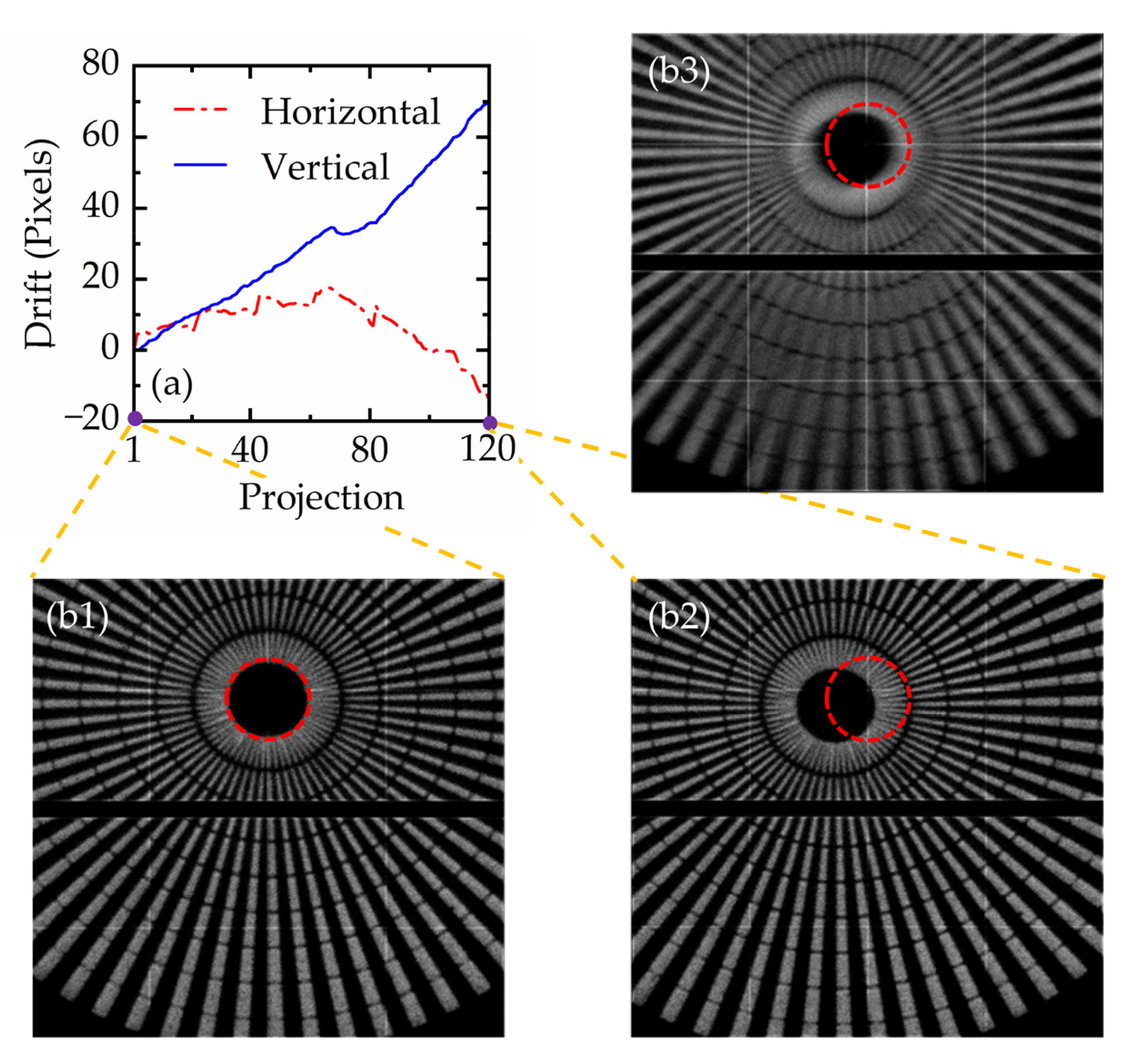
2. Necessity for Projection Drift Correction in Nano-CT

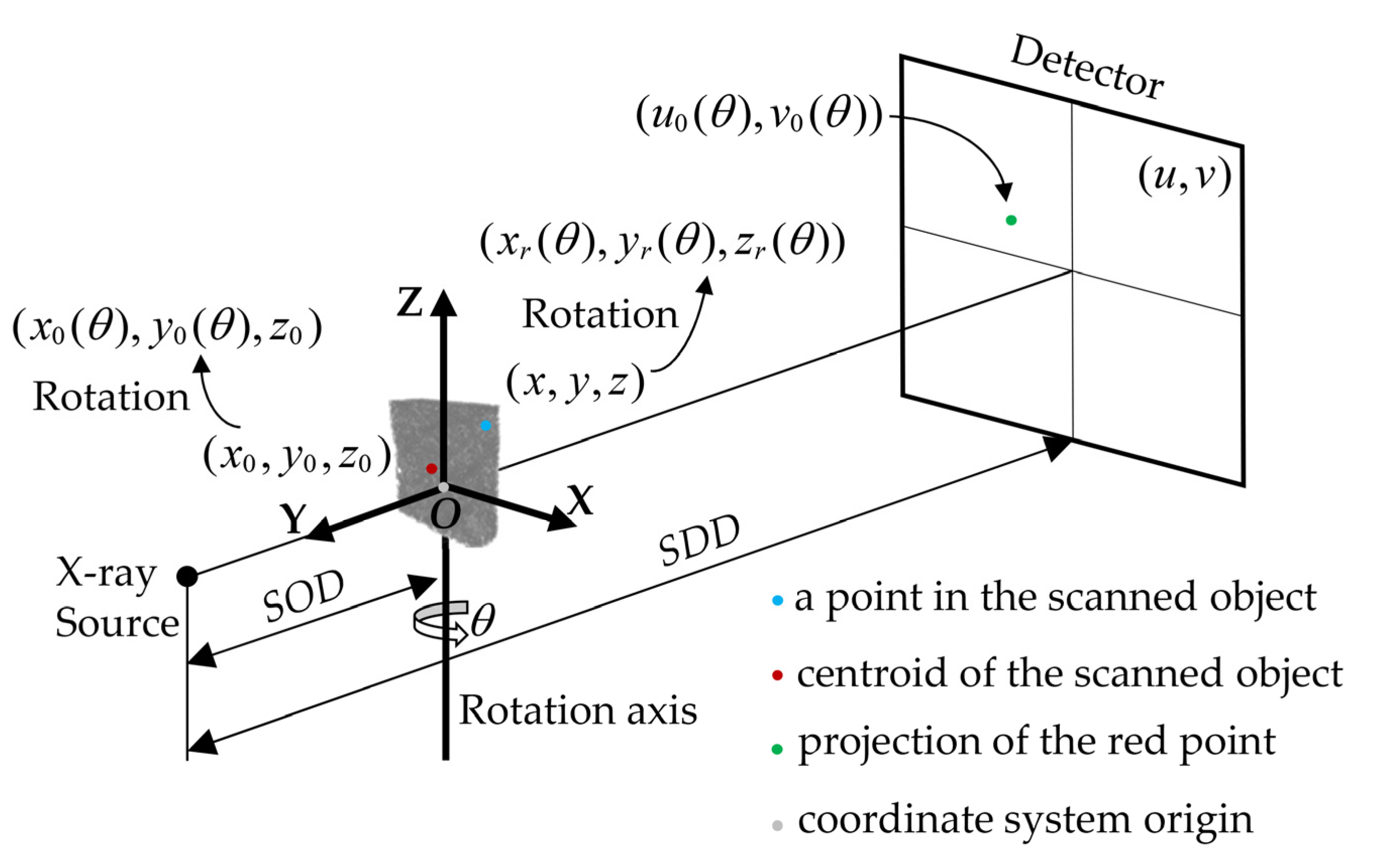
Long scanning in nano-CT can lead to instability of the system and the object, which causes projection drift. Previous studies have demonstrated that projection drift is a rigid motion parallel to the detector plane [2,13,15]. In this section, we show the necessity of projection drift correction in nano-CT through the fixed-angle scanning experiment of a Siemens star and the partial derivative analysis of the projection position.

Table 1. The detailed parameters of nano-CT and scanning parameters of a Siemens star.

	System Parameter	Value
X-ray tube	Voltage	60 kV
	Current	0.3 mA
Detector	Pixel size	75 μm
	Detector size	1030 × 1065 pixels
Siemens star Scanning	Projection number	120
	Exposure time	30 s

provides the system parameters summarized by the manufacturer and the scanning parameters of a Siemens star. Nano-CT operates at 60 kV and 0.3 mA. The detector size was 1030 × 1065 pixels and the pixel size was 75 μm. The Siemens star took 120 projections at the same angle with an exposure time of 30 s. The results of the fixed-angle scanning experiment are shown in Figure 1, where the drift during the scanning and the projections of the Siemens star are provided. To record the drift during scanning, the first projection was used as the baseline. The deviations between the subsequent projections and the first projection were calculated by a single-step DFT algorithm [27], and the projection drift is shown in Figure 1a. The result shows that the projection drift was continuous, slow, and smooth, without sudden movements. The first and last (120th) projections of the Siemens star are displayed in Figure 1(b1,b2), respectively. Figure 1(b3) shows the average image of the 120 projections. The last projection shown in Figure 1(b2) is off-centered with respect to the first projection in Figure 1(b1), which indicates that the drift causes serious misalignment of the projections, and the drift occurs in both horizontal and vertical directions. In addition, Figure 1(b3) shows that the average projection had serious blurs. Similarly, the direct accumulation of these projections via back-projection process resulted in a degradation of the reconstruction results. Therefore, it was necessary to correct the projection drift in order to achieve the achievable spatial resolution of nano-CT. Furthermore, Figure 1 clearly shows the difference between the projection drift of nano-CT and the geometric artifacts. Geometric artifacts are caused by the fixed errors of projections due to the non-ideal geometric relation of the hardware system. However, the drift artifacts are caused by the projection drift due to the instability of the system and the object. The projection drift is random, i.e., it is a variable function, not a fixed value.

In addition, the necessity of nano-CT drift correction is also shown through partial derivative analysis. To describe the cone-beam nano-CT system, we introduce the Cartesian coordinate system, as shown in Figure 2. All equations were derived based on the coordinate system of Figure 2. Under ideal conditions, the object only moves according to the set scanning trajectory, and the object is only rotated by the rotation axis. Under the cone-beam imaging geometry with circular trajectory, the spatial position of any point in the imaged object during the rotation process should satisfy the following:

$$\left(\begin{array}{c}{x}_r(\theta )\\ y_r(\theta )\\ z_r(\theta )\end{array}\right)=\left(\begin{array}{ccc}\cos (\theta )& \sin (\theta )& 0\\ -\sin (\theta )& \cos (\theta )& 0\\ 0& 0& 1\end{array}\right)\left(\begin{array}{c}x\\ y\\ z\end{array}\right),$$

(1)

where $(x,y,z)$ is the coordinate of a point in the imaged object, and $(x_r(\theta ),y_r(\theta ),z_r(\theta ))$ is the rotation coordinate of $(x,y,z)$ at the rotation angle $\theta$.

The object was scanned via X-ray and projection was formed on the detector. The projection position of the $(x_r(\theta ),y_r(\theta ),z_r(\theta ))$ should satisfy the following:

$$\left\{\begin{array}{l}u=\frac{x_r(\theta )}{SOD+y_r(\theta )}SDD\\ v=\frac{z}{SOD+y_r(\theta )}SDD\end{array}\right..$$

(2)

To analyze the influence of horizontal position, vertical position, and source-to-detector distance ($SDD$), partial derivative analysis was conducted on the projection coordinates in (2).

$$\begin{array}{cc}\frac{\partial (u)}{\partial x_r}\approx M& \frac{\partial (u)}{\partial SDD}\approx 0\\ \frac{\partial (v)}{\partial x_r}=0& \frac{\partial (v)}{\partial SDD}\approx 0\end{array}\begin{array}{cc}& \frac{\partial (u)}{\partial z}=0\\ & \frac{\partial (v)}{\partial z}\approx M\end{array},$$

(3)

where M is the magnification ratio. The magnification ratio is related to the SOD and SDD as follows: $M=\raisebox{1ex}{$SDD$}\!\left/ \!\raisebox{-1ex}{$SOD$}\right.$. Partial derivative analysis suggests that the change in the position of the object in the 3D space (or the change in the relative position between the object and the nano-CT) affects the position of the projection. Specifically, the horizontal drift causes the projection to move horizontally ($u$), and the vertical drift causes the projection to move vertically ($v$). The change in the scaling distance had a minor effect on the projection position and can be ignored.

Two conclusions can be drawn according to (3). Firstly, the scanned object was located extremely close to the source because nano-CT provides high geometric magnification. A slight movement of the focus spot, mechanical expansion, and motion of the object can cause serious misalignment of the projections. Therefore, it is necessary to perform drift correction. Secondly, the centroid, as an inherent feature of the object, had the same drift with the object. Therefore, the projection drift of the centroid can be measured instead of the drift of the scanned object.

3. Theory

Wang et al. [25] derived the trajectory of geometric moments of projections in parallel-beam CT to correct the vibration of TXM. In their study, the trajectory of geometric moments proved to be a sine function of the rotation angle in the horizontal direction and a constant in the vertical direction. Trajectories need to be re-derived due to geometric differences between the parallel beam and the cone beam.

In this section, the horizontal coordinate curve of TPC (H-TPC) and the vertical coordinate curve of TPC (V-TPC) in cone-beam CT are derived. In addition, to further explore the principle of the proposed method, the consistency between the PTOC and TPC is considered. The results show that the TPC is consistent with the PTOC. Therefore, the TPC contains the motion law of the object centroid, which is also the reason why TPC is used for the correction of projection drift.

3.1. Measurement of PTOC

Similar to TPC, the horizontal (H-PTOC) and vertical coordinate curves (V-PTOC) of PTOC are derived. An object scanned by the nano-CT is considered. The centroid coordinate of the scanned object can be written as the following:

$$\begin{array}{l}{x}_0=\frac{{\displaystyle \iiint xf(x,y,z)dxdydz}}{{\displaystyle \iiint f(x,y,z)dxdydz}}\\ y_0=\frac{{\displaystyle \iiint yf(x,y,z)dxdydz}}{{\displaystyle \iiint f(x,y,z)dxdydz}},\\ z_0=\frac{{\displaystyle \iiint zf(x,y,z)dxdydz}}{{\displaystyle \iiint f(x,y,z)dxdydz}}\end{array}$$

(4)

where $f(x,y,z)$ is the attenuation function of the object, $\left(x_0,y_0,z_0\right)$ is the centroid of the scanned object.

The centroid here is a generalized concept, which represents the center of the attenuation coefficient. $(x_0(\theta ),y_0(\theta ),z_0)$ represents the position of the object centroid during rotation. Based on (2), the projection of the object centroid becomes the following:

$$\begin{array}{c}{u}_0(\theta )=\frac{x_0(\theta )}{SOD+y_0(\theta )}SDD\\ v_0(\theta )=\frac{z_0}{SOD+y_0(\theta )}SDD\end{array},$$

(5)

where $u_0(\theta )$ and $v_0(\theta )$ are the H-PTOC and V-PTOC, respectively.

Based on (1) and (5), the H-PTOC and V-PTOC can be expressed as:

$$\begin{array}{c}{u}_0(\theta )=\frac{x_0\cos (\theta )+y_0\sin (\theta )}{SOD+(y_0\cos (\theta )-x_0\sin (\theta ))}SDD\\ v_0(\theta )=\frac{z_0}{SOD+(y_0\cos (\theta )-x_0\sin (\theta ))}SDD\end{array}.$$

(6)

3.2. Measurement of TPC

We assume that the geometrical parameters of the nano-CT system shown in Figure 2 have been calibrated. If random factors (drift, jitter, etc.) are not considered, the projection can be expressed as an integral of the attenuation coefficient of the object based on (1) and (2),

$$p_{\theta }(u,v)={\displaystyle \iiint f(x,y,z)}\delta (\frac{x_r(\theta )}{SOD+y_r(\theta )}SDD-u,\frac{z}{SOD+y_r(\theta )}SDD-v)dxdydz,$$

(7)

where $p_{\theta }(u,v)$ is the projection at the rotation angle $\theta$. u and v are the horizontal and vertical positions on the detector, respectively.

We define $m_u(\theta )$ and $m_v(\theta )$ as the H-TPC and V-TPC, respectively. Then, we have the following:

$$\begin{array}{c}{m}_u(\theta )=\frac{{\displaystyle \iint u{p}_{\theta }(u,v)dudv}}{{\displaystyle \iint p_{\theta }(u,v)dudv}}\\ m_v(\theta )=\frac{{\displaystyle \iint v{p}_{\theta }(u,v)dudv}}{{\displaystyle \iint p_{\theta }(u,v)dudv}}\end{array}.$$

(8)

Based on (1), (4), (7), and (8), the H-TPC and V-TPC can be written as the following:

$$\begin{array}{c}{m}_u(\theta )=\frac{x_0\cos (\theta )+y_0\sin (\theta )}{SOD+(y_0\cos (\theta )-x_0\sin (\theta ))}SDD\\ m_v(\theta )=\frac{z_0}{SOD+(y_0\cos (\theta )-x_0\sin (\theta ))}SDD\end{array}.$$

(9)

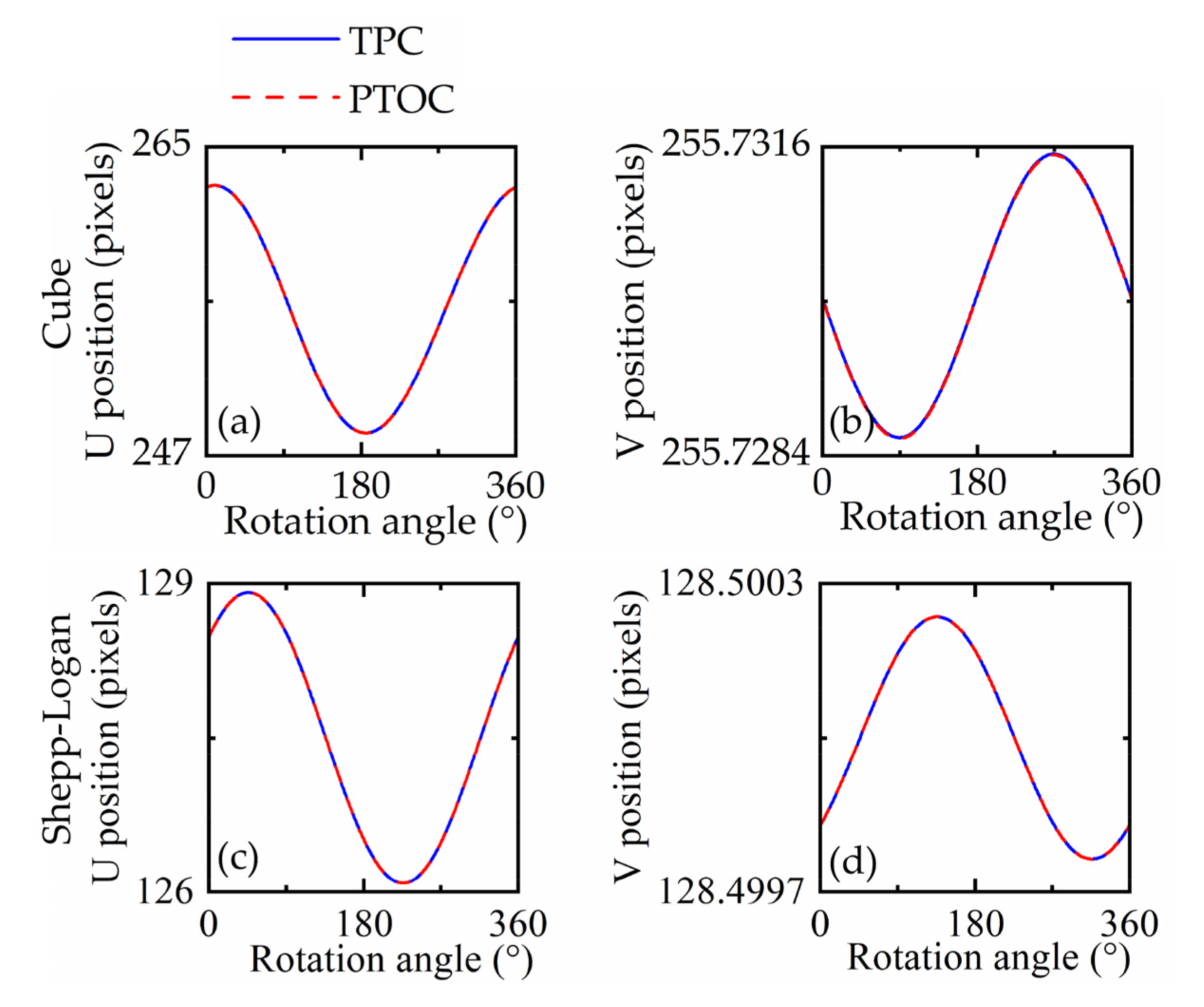
3.3. Consistency between TPC and PTOC

By comparing (6) and (9), it can be inferred that the TPC is equal to the PTOC. This indicates that the PTOC can be replaced by TPC, so the projection drift occurring in the scanning process can be calculated by TPC. We conducted two simulation scanning experiments on a cube and Shepp–Logan phantom. The parameters of the simulation experiments are given in

Table 2. Parameters of the simulation phantoms.

Phantom	Object Size (mm)	Detector Size (mm)	SOD (mm)	SDD (mm)	Centroid Position (mm)
					x	y	z
Cube	2.56 × 2.56 × 2.56	256 × 256	588.00	600.00	1.30	1.30	1.30
Shepp–Logan	64.00 × 64.00 × 64.00	512 × 512	300.00	600.00	33.90	32.33	32.18

.

Figure 3 shows the TPC (H-TPC and V-TPC) and the PTOC (H-PTOC and V-PTOC), which confirms the above derivation; i.e., our method is equivalent to correcting the object centroid. In addition, we used the SSE to evaluate the similarity of the TPC and the PTOC. The numerical results are shown in

Table 3. The similarity measures between TPC and PTOC. In the horizontal direction (U), the SSE between H-TPC and H-PTOC is calculated. In the vertical direction (V), the SSE between V-TPC and V-PTOC is calculated.

Direction	SSE
	Cube	Shepp–Logan
Horizontal (U)	2.0248 × 10−23	3.6488 × 10−8
Vertical (V)	3.4294 × 10−16	3.5077 × 10−8

. The results show a good fitting between the trajectories.

4. Method

Our method can be summarized as follows. Firstly, the TPC is fitted by Section 4.1. Secondly, the horizontal and vertical drifts of each projection are estimated using the fitted TPC as the baseline. Finally, discrete Fourier transform (DFT) is used to translate the projections in a subpixel manner. The corrected projections are reconstructed using the Feldkamp, Davis and Kress (FDK) algorithm [28]. When fitting the TPC, considering the influence of drift asymmetry on the fitting error, the sliding window-based SSE minimization method is used to find the partial projection set (optimal interval) with the most stable drift, and the projection set is used to estimate the complete trajectory. To improve the applicability of the method, the interval search method is used to calculate the drift when the projection is not completely within the field of view of the detector. The correction flow diagram is shown in Figure 4.

4.1. Fitting the Complete TPC

The proposed method first finds the projection set (interval) with the most stable drift and uses the partial TPC in this interval to estimate the complete TPC. The estimated H-TPC and V-TPC are represented by $m_u(\theta )$ and $m_v(\theta )$, respectively. When drift occurs, the ideal TPC fluctuates randomly. $u_{\theta }$ and $v_{\theta }$ represent the drift in horizontal and vertical direction at the angle $\theta$, and the TPC with drift can be expressed as:

$$\begin{array}{c}{m}^{\prime }{}_u(\theta )=\frac{{\displaystyle \iint (u+u_{\theta })p_{\theta }(u,v)dudv}}{{\displaystyle \iint p_{\theta }(u,v)dudv}}\\ m^{\prime }{}_v(\theta )=\frac{{\displaystyle \iint (v+v_{\theta })p_{\theta }(u,v)dudv}}{{\displaystyle \iint p_{\theta }(u,v)dudv}}\end{array},$$

(10)

where $m^{\prime }{}_u(\theta )$ and $m^{\prime }{}_v(\theta )$ are H-TPC and V-TPC containing drift, respectively. Therefore, the TPC with drift deviates from ideal trajectories which are deduced in (9). Our aim was to find a relatively stable projection set to estimate the complete TPC. The closer the TPC estimated by the projection set to (9), the more stable these projections are. When estimating the complete trajectory, the projection sets used by H-TPC and V-TPC are different, but the method of projection set determination is the same. Therefore, here we use TPC to represent H-TPC and V-TPC to simplify the expression. The process of determining the optimal projection set is divided into three steps. (1) A sliding window is used and the partial TPC is measured within the sliding window; (2) the partial TPC measured in (1) is fitted (the least-squares method) using (9) and the SSE between the fitted TPC and the measured TPC is calculated; (3) the projection set within the sliding window corresponding to the minimum value of the SSE is considered to be optimal. Then, the optimal projection set is used to estimate the complete TPC.

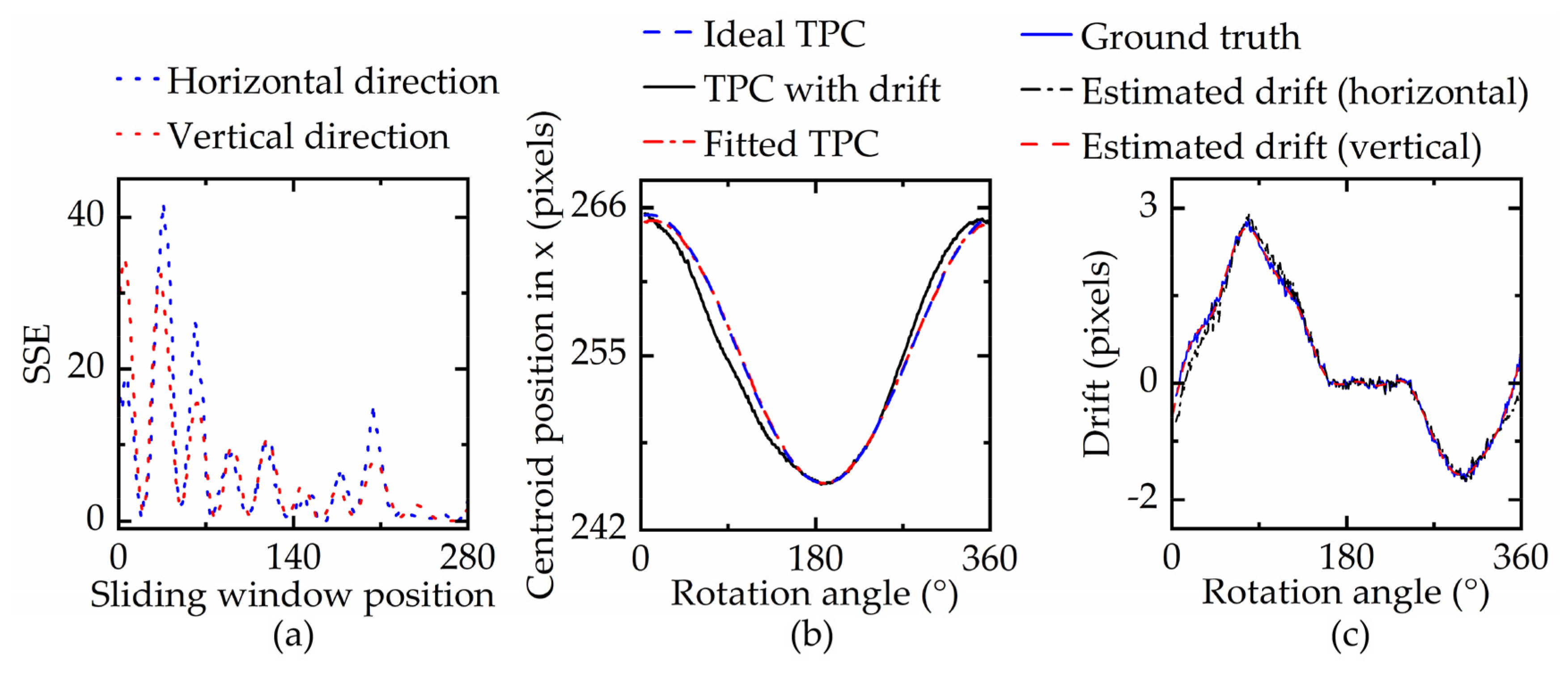
4.2. Interval Search Method for Estimating the Drift

After confirming the complete TPC, the projection drift is estimated. Based on (8) and (10), the horizontal drift ($u_{\theta }$) and vertical drift ($v_{\theta }$) can be written as the following:

$$\begin{array}{c}{u}_{\theta }=m^{\prime }{}_u(\theta )-m_u(\theta )\\ v_{\theta }=m^{\prime }{}_v(\theta )-m_v(\theta )\end{array}.$$

(11)

However, (11) is valid only for untruncated projections; i.e., the projection is completely within the imaging field of the detector. In the case of projection truncation due to drift, we propose an interval search method to calculate the drift.

When truncation occurs, the drift can be estimated by moving the projections to match the fitted TPC. A fixed interval $\left[a,b\right]$ is set first, and then the projections are supplemented with the edge line because the projections are concatenated and vary very little over a small range. The search step determines the estimation accuracy of drift. To achieve sub-pixel accuracy, we choose 0.1 pixels as a step. $c_k\left(\theta \right)$ is the centroid of projection $p_{\theta }(u,v)$ moving $k$ pixels. $c(\theta )$ is the value of the fitted TPC at rotation angle $\theta$. Our goal is to minimize the trajectory error $\Delta \left({\theta }_k\right)$. Then, the $k$ which minimizes the trajectory error $\Delta \left({\theta }_k\right)$ is considered to be the drift value of this rotation angle $\theta$.

$$\begin{array}{c}\Delta \left({\theta }_k\right)=c_k\left(\theta \right)-c(\theta )\\ \min ((\Delta {\theta }_k))\end{array}.$$

(12)

The estimation of projection drift in the case of projection truncation caused by drift is a crucial challenge in self-correction methods because the information beyond the detector is unknown. The interval search method performs well when the shape of the object does not change dramatically and the drift is less than the number of supplementary rows (columns) in projections. However, if the projection truncation occurs when the shape of the object changes dramatically or when the amount of drift is too large, this method cannot effectively improve blurring in reconstructed slices.

5. Experiments

5.1. Simulation Study

A Shepp–Logan phantom built in the Cartesian coordinate system in Figure 2 was used to evaluate the proposed method. The phantom had a size of 256 × 256 × 256 pixels and was composed of several ellipsoids of different sizes. In the simulation, the phantom was projected using the cone-beam CT projection simulation program. The virtual detector size was set as 512 × 512 pixels with a size of 750 × 750 nm² for each pixel. The number of projections was 360, and the rotation step was 1°. The actual drift of the nano-CT was added to the simulation projections as the ground truth. The working environment was MATLAB 2016b, and the CPU was an Intel Xeon Gokd.5118@2.3GHz, RAM 128 GB, 64 bit.

Firstly, the correction process and results of the proposed method are shown. Secondly, the anti-noise performance of the proposed method is considered. Three levels (5%, 10%, and 15%) of noise are added to test the correction effect of the proposed method. Thirdly, the adaptability of the method for different drift levels is examined. The simulation is performed at five sets of different drift levels, which are 2 times, 4 times, 6 times, 8 times, and 10 times the actual drift levels. The deviation between the estimated result and the ground truth is calculated. Then, the causes of the calculation error are analyzed.

5.2. Tomato Seed and Bamboo Stick Imaging

Nano-CT is of great significance for accurately evaluating the 3D morphology inside seeds and predicting the germination potential [29]. The proposed correction method is applied to our nano-CT system (see Table 1). The projection size is 1065 × 1030 pixels with a pixel size of 750 × 750 nm².

The tomato seeds and bamboo sticks are scanned by 1440 projections. The exposure time is 13 s, and the rotation step of the turntable is 0.25°. The total working time of nano-CT is 10.5 h.

5.3. Comparative Approaches

Global fitting and RSM are compared to our method. Global fitting is a common centroid-based self-correction method. In previous studies, the centroid of sinogram and the equivalent idea of TPC were used to correct the horizontal vibration of the second generation of CT and the axial vibration of parallel-beam CT, respectively. Global fitting can effectively eliminate the vibration of individual projection angles. However, projection drift of nano-CT occurs in the whole scanning process, and direct global fitting can still lead to trajectory deformation. In our experiment, the global fitting method based on geometric moments [25] is compared with the proposed method.

RSM uses a short reference scan to align the original projections. In our experiment, immediately after obtaining the original projections, we continued to scan the object at 10 times the rotation step to obtain the sparse reference projections. The single-step DFT algorithm [27] is used to align the original projections with the reference projections to estimate the drifts. Finally, cubic spline interpolation is used to estimate the remaining drifts.

6. Results and Discussion

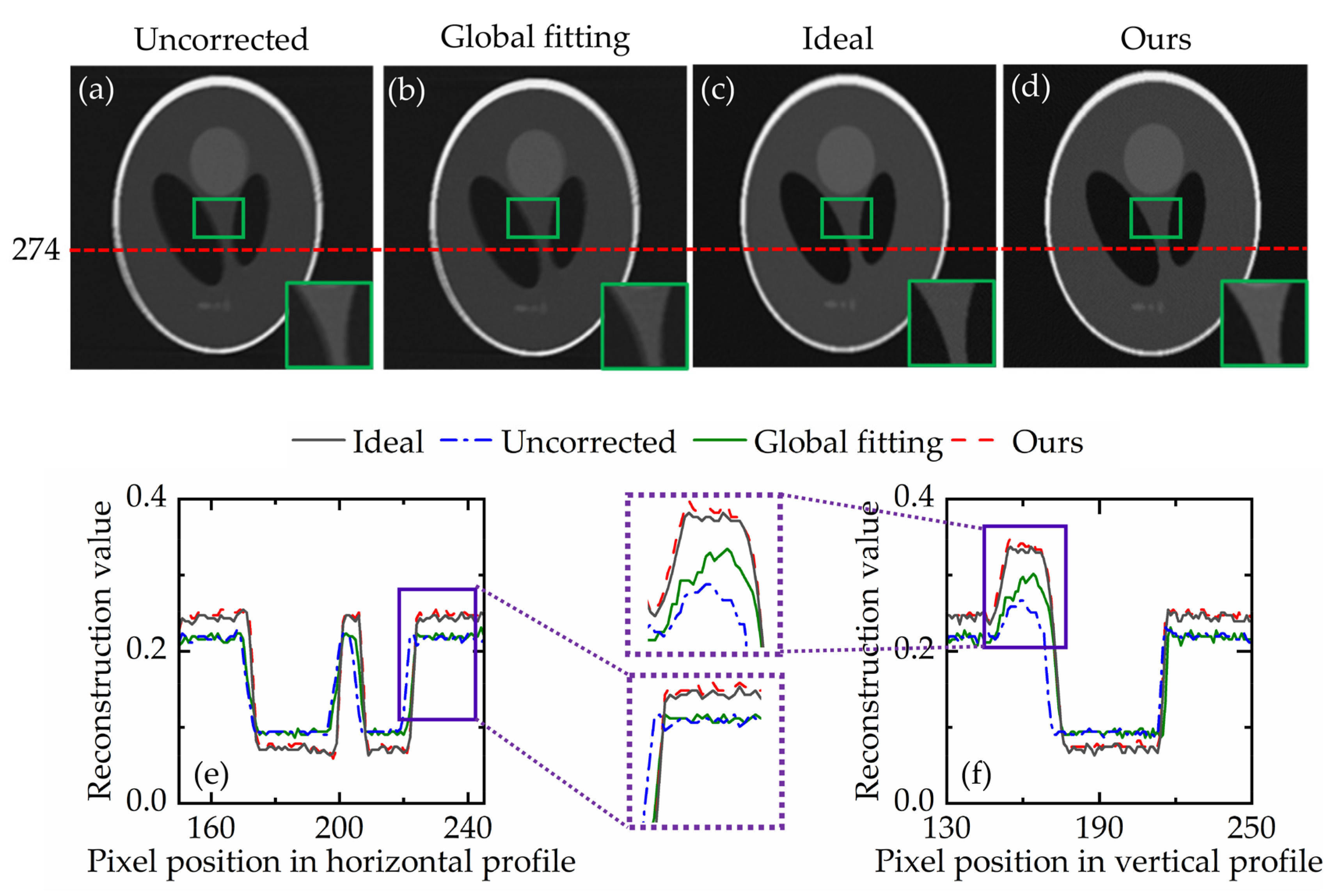
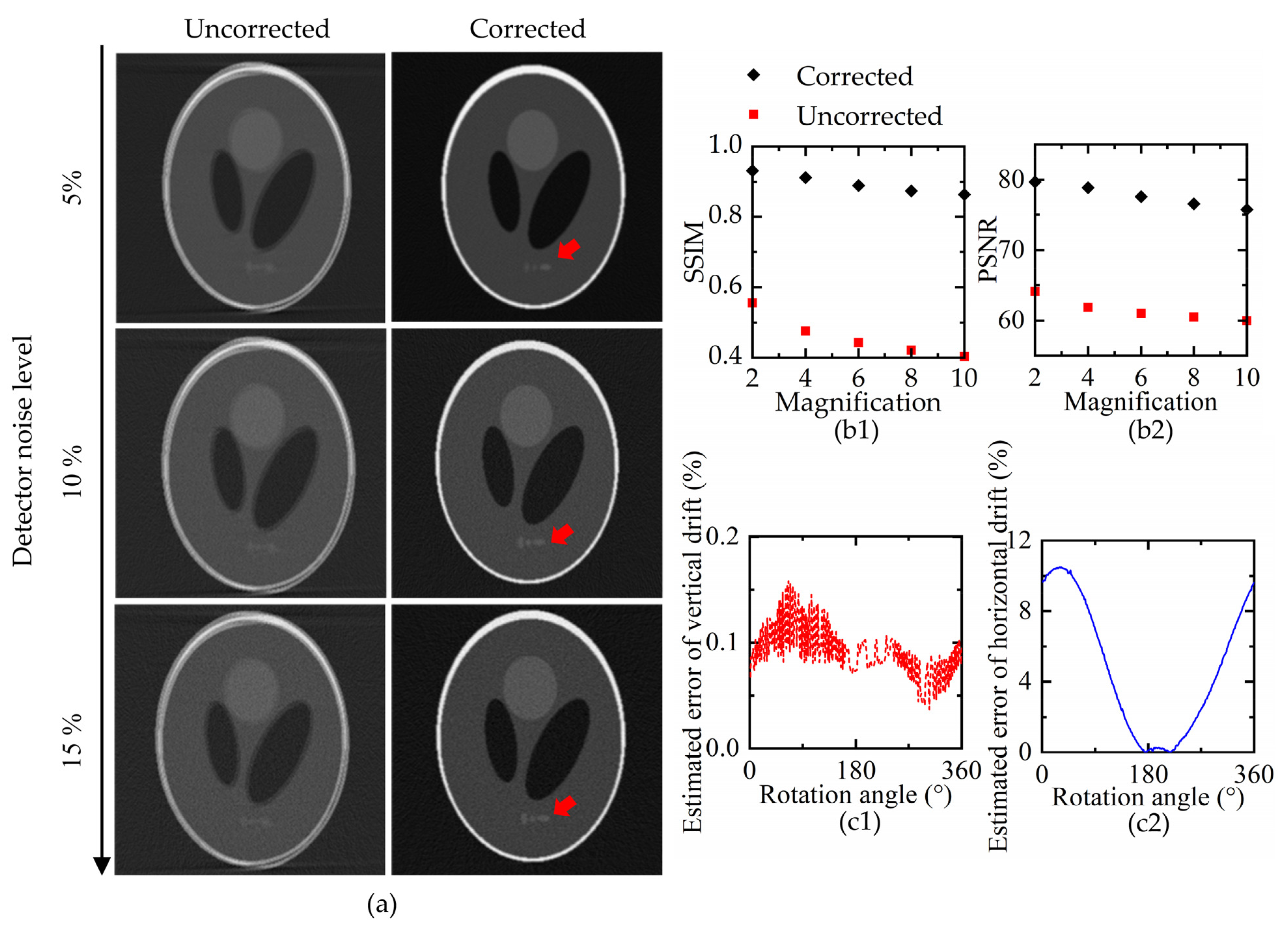
6.1. Simulation Result

The correction process and estimated drift of the proposed method are shown in Figure 5. Firstly, the actual drift measured by nano-CT is added in the vertical and horizontal directions, as shown in the blue curve of Figure 5c. The range of ground truth is from −1.5 pixels to 3 pixels. Secondly, the process of determining the optimal interval (projection set) is shown in Figure 5a. The length of the sliding window is 80. The fitted TPC is calculated at each position of the sliding window. The position of the optimal interval can be obtained by minimizing the SSE between the fitted results (by (9)) and the measured TPC in the sliding window. The smallest SSE occurs at the sliding window position with sequence No. 164; i.e., projections 164 to 243 form the optimal projection set. Then, the partial TPC in the optimal interval is used to estimate the complete trajectory, as shown in the red curve in Figure 5b. The TPC with drift (black curve in Figure 5b) has an obvious deviation from the ideal trajectory due to the unaligned projections, while the TPC corrected by the proposed method almost coincides with the ideal trajectory. Finally, the difference between the fitted trajectory (red curve in Figure 5b) and the measured trajectory (black curve in Figure 5b) is used to estimate drifts, which are shown below in Figure 5c. The results show that the proposed method can effectively correct the projection drifts in both vertical and horizontal directions.

Figure 6 shows the reconstructed slices corrected via different methods. Here, Figure 6a–d displays the uncorrected reconstructed slice, reconstructed slice with global fitting correction, ideal reconstructed slice, and the reconstructed slice with our method, respectively. The uncorrected slice shows distinct double edge artifacts due to the projection misalignment. The global fitting correction of the centroid is effective when the jitter and drift are uniform. However, in the actual case (blue curve in Figure 5c), the drift is not uniform, so global fitting cannot achieve significant correction. The reconstructed slice (Figure 6d) corrected by our method is visually identical to the ideal one (Figure 6c), and it is difficult to visually differentiate them. There are no obvious blurs and artifacts in the slice, though there is a slight deviation between the estimated results and the ground truth, as shown in Figure 5c. Figure 6e,f shows the horizontal and vertical profiles of the slices in Figure 6a–d, respectively. The uncorrected profile is higher than the ideal contour in the low gray value area, and it is lower than the ideal profile in the high gray value area. This is because the misalignment of the projections causes a dispersion of the reconstructed value of the highlighted area during reconstruction.

Table 4. EOG and SSIM in Figure 6a–d.

Reconstructed Slice	EOG	SSIM
Uncorrected	0.641	0.708
Global fitting	0.794	0.852
Ideal	1.000	1.000
Ours	0.859	0.967

shows the normalized energy of gradient (EOG) and structural similarity index (SSIM) [30] of Figure 6a–d. EOG and SSIM show that the corrected result of our method can effectively approximate the ideal slice. Compared to global fitting, the numerical evaluation index of the proposed method is improved by 9%.

In addition, we analyze the performance of the proposed method in two complex cases. Firstly, the different noise levels (5%, 10%, and 15%) are added to the projections to test the noise resistance of the proposed method. Here, we add Poisson distributed noise to simulate the actual situation on the detector [31], and the detector noise level represents the ratio of noise to the sum of gray projection values. The corrected slices in Figure 7a show that the proposed method achieves a clear correction effect in different noise levels. Secondly, the effect of the magnitude of the drift on the proposed method is considered. We use five sets of original drift multiples (2 times, 4 times, 6 times, 8 times, and 10 times) to gradually examine the correction effect, and the maximum amplitude of drift is 27 pixels. Figure 7(b1,b2) shows the SSIM and the peak signal-to-noise ratio (PSNR) at different drift levels, respectively. When the drift is greater than 27 pixels, the method can still improve the image quality. Then, the estimation errors are evaluated in the case of the maximum drift amplitude (10 times of the ground truth), as shown in Figure 7(c1,c2). The vertical error is very small. Further, the horizontal error is much larger than the vertical error. Because the trajectory range of V-TPC is very small, the estimation error of the complete trajectory is small. The amplitude of H-TPC varies greatly, and the estimated trajectory at rotation angles far away from the optimal projection set is not more accurate than V-TPC. Thus, the horizontal error appears in the drift estimation. However, as previously analyzed, even in the case where the drift level is up to 27 pixels, the horizontal drift error reaches 12%, and there is no visual impact on the slices.

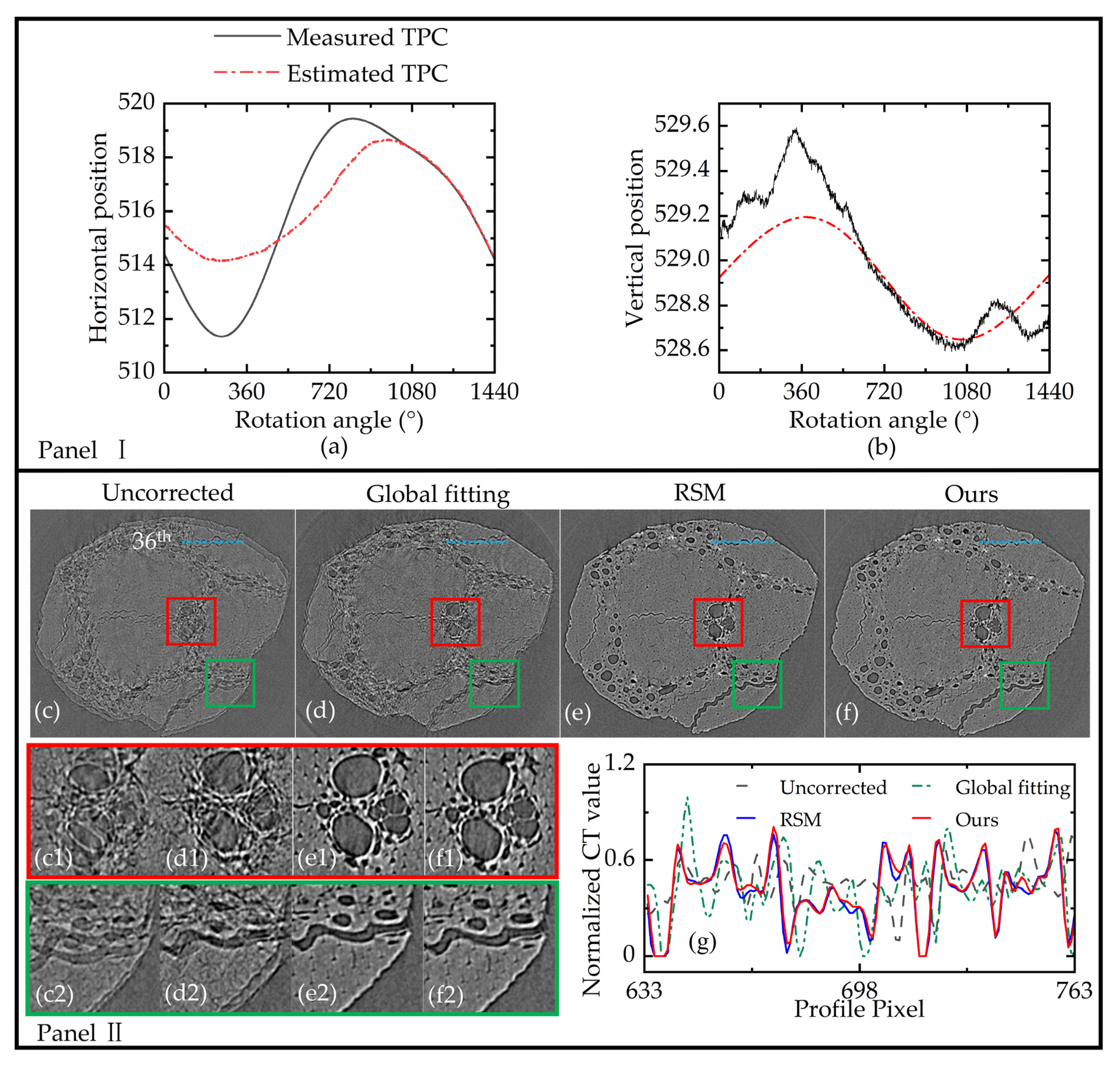
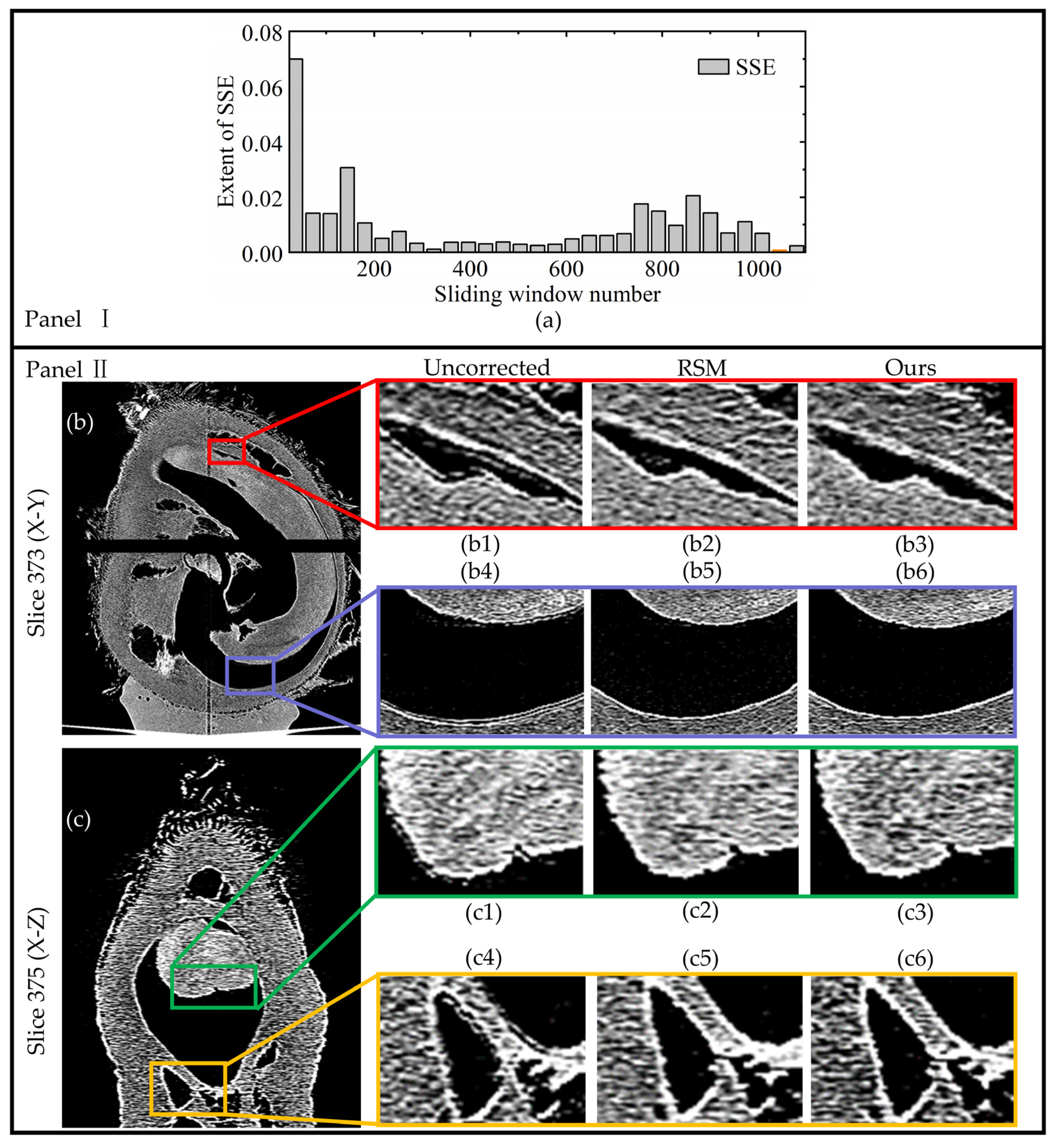
6.2. Practical Experiment

Figure 8 shows the experimental results of bamboo stick scanning. The measured TPC and estimated TPC are shown in Panel I of Figure 8. The red curve is the trajectory estimated by the optimal projection interval, and the black curve is the measured trajectory calculated from the original projections.

The corrected projections are used for the reconstruction of the bamboo stick. The reconstructed slices via different correction methods are shown in Panel II of Figure 8. The uncorrected slice (Figure 8(c,c1,c2)) contains serious artifacts, especially at the edge. This kind of artifact causes the fine structure information to be indistinguishable, which makes the measurement difficult. Figure 8(d,d1,d2) shows the correction results of the global fitting method. The detailed parts of the bamboo stick (e.g., small holes) still contain severe blurring because the asymmetry of drift leads to the inaccurate estimation of the TPC. Nevertheless, the image quality of the slices is improved compared to the uncorrected slices. The performance of the proposed method (Figure 8(f,f1,f2)) is comparable to that of the RSM (Figure 8(e,e1,e2)). The edge sharpness of the slice is significantly enhanced, the double edge artifacts is removed, and the image quality is greatly improved after the correction. The profile of the reconstructed slice is used to evaluate the reconstruction quality. Figure 8g shows the profile of the bamboo stick marked with a blue line in Figure 8c–f. The results obtained through the use of our method are close to those obtained via RSM. Furthermore, the proposed method does not require extra scanning and saves at least 1872 s (the sum of exposure times for reference projections).

In addition, we also scan the tomato seed, which has more detail. The correction results for the tomato seed are shown in Figure 9. Panel I of Figure 9 shows the process of obtaining stable interval and the drift estimation results. We divide 1440 projections into 1080 projection intervals. Figure 9a shows the SSE of the fitting curve, and the valley value appears in the 1080th interval.

The reconstructed slices of tomato seed are shown in Panel II of Figure 9. The 373rd and 375th slices are shown on the X-Y and X-Z planes, respectively. The second column in Panel II (b1, b4, c1, c4) represents the original slices containing artifacts. The original slices have distinct double-edge artifacts and blurring. Column 3 (b2, b5, c2, c5) and column 4 (b3, b6, c3, c6) are the corrected results obtained via the RSM and our method, respectively. Compared to the uncorrected slices, the corrected slices are significantly improved. Our corrected slices are similar to those obtained via RSM. In addition, our method avoids extra scanning.

Figure 8 and Figure 9 show the reconstructed slices corrected via the different methods. The results of our method and RSM are very similar visually. Numerical evaluation is used to further assess the performance of the proposed method and RSM. On the one hand, the reconstructed slices with drift artifacts are blurry. On the other hand, there is no ground truth of reconstructed slices in the practical scanning. Thus, two image evaluation functions without reference (Vollath function [32] and image entropy) are considered. Vollath function is a classical image sharpness evaluation function based on self-correlation, which can be expressed as follows:

$$Vollath={\displaystyle \sum _M{\displaystyle \sum _{N}f\left(x,y\right)\left|f\left(x+1,y\right)-f\left(x+2,y\right)\right|}},$$

(13)

where $f\left(x,y\right)$ is the reconstructed slice. $M$ and $N$ represent the length and width of the reconstructed slice, respectively. The difference between adjacent pixels of a clear image is large, so the Vollath function is larger. Entropy is an index to measure the amount of information contained in an image. Therefore, the sharp images have greater entropy.

Since the Vollath function and entropy have different orders of magnitude, we normalize the indexes by the maximum value obtained by different methods. The normalized evaluation results are listed in

Table 5. A numerical analysis of the correction results (our method and RSM) in Figure 8 and Figure 9.

Method	RSM						Ours
Sample	Bamboo Stick		Tomato Seed				Bamboo Stick		Tomato Seed
Number	1	2	1	2	3	4	1	2	1	2	3	4
Vollath	1.000	0.940	0.991	0.971	1.000	1.000	0.927	1.000	1.000	1.000	0.935	0.920
Entropy	1.000	0.993	1.000	1.000	1.000	0.979	0.992	1.000	0.995	0.990	0.998	1.000

. The “number” in Table 5 represents the line number of the local enlarged image in the result images (Figure 8 and Figure 9). The mean of the scores for the two methods listed in Table 5 is calculated. It is observed that the score of the proposed method is 99.0% of the RSM score. Therefore, the correction effect achieved by the proposed method is 99.0% of what was achieved via RSM, and the proposed method saves 10% of the scanning time in practical scanning because no additional scanning is required.

7. Conclusions

We propose a self-correction strategy for the drift artifacts of cone-beam nano-CT which does not require iteration, auxiliary correction phantoms, and reference projections. The technique is based on the invariance of the TPC. The simulation study shows that the corrected slices can still maintain a high resolution when the noise of the detector increases, which indicates that the correction strategy is not sensitive to noise. In addition, the technique has been applied to a practical laboratory cone-beam nano-CT system, and the reconstructed slices are close to those obtained via RSM.

The study provides a convenient and efficient method to correct the misalignment of projections, which has two advantages compared to the traditional centroid-based correction [24,25]. Firstly, the search process based on the SSE of the stable drift interval ensures the accuracy of the correction. The search process removes the sharp drift change region and only uses the stable drift range for fitting. Secondly, the interval search algorithm is used to improve the accuracy of drift estimation in the case of projection truncation due to drift.

The proposed technique is compared to the RSM through scanning experiments on tomato seed and bamboo stick. The reconstruction slices show that they have similar performance, and it is difficult to find any difference in the corrected slices via observation. The image evaluation indexes show that the proposed method achieves a 99.0% RSM correction effect. However, the proposed correction strategy does not require the reference scan, which improves the correction efficiency.

It may be noted that the technique has some limitations. First, if the drift is particularly severe throughout the scan (although this is not common), the accuracy of our method may decrease because a stable interval is required. Second, the proposed self-correction is effective for the projections completely within the detector (or projection truncation due to drift). When scanning the region of interest, the method is not applicable because the TPC is unknown in this case.

Overall, the proposed method has the advantages of short computation time, low operation complexity, high correction efficiency, and low experimental cost. At the same time, it has excellent anti-noise performance. The technique can be applied to cone-beam nano-CT, which can eliminate the blur caused by drift to obtain satisfactory results. In addition, the technique is also applicable for random jitter correction in the scanning process because random jitter can itself be regarded as a sparse drift.

References

1. Guo, E.; Zeng, G.; Kazantsev, D.; Rockett, P.; Bent, J.; Kirkland, M.; Van Dalen, G.; Eastwood, D.S.; StJohn, D.; Lee, P.D. Synchrotron X-ray tomographic quantification of microstructural evolution in ice cream—A multi-phase soft solid. RSC Adv. 2017, 7, 15561–15573. [Google Scholar] [CrossRef] [Green Version]
2. Vogeler, F.; Verheecke, W.; Voet, A.; Kruth, J.P.; Dewulf, W. Positional stability of 2D X-ray images for computer tomography. In Proceedings of the International Symposium of Digital Industrial Radiology and Computed Temography, Berlin, Germany, 20–22 June 2011. [Google Scholar]
3. Hiller, J.; Maisl, M.; Reindl, L. Physical characterization and performance evaluation of an x-ray micro-computed tomography system for dimensional metrology applications. Meas. Sci. Technol. 2012, 23, 085404. [Google Scholar] [CrossRef]
4. Reisinger, S.; Schmitt, M.; Voland, V. Geometric adjustment methods to improve reconstruction quality on rotational cone-beam systems. In Proceedings of the 4th Conference on Industrial Computed Tomography (iCT), Wels, Austria, 19–21 September 2012. [Google Scholar]
5. Flay, N.; Sun, W.; Brown, S.; Leach, R.; Blumensath, T. In Investigation of the Focal Spot Drift in Industrial Cone-beam X-ray Computed Tomography. In Proceedings of the Digital Industrial Radiology and Computed Tomography (DIR 2015), Ghent, Belgium, 22–25 June 2015. [Google Scholar]
6. Cho, Y.; Siewerdsen, D.M.J.; Jaffray, D. Accurate technique for complete geometric calibration of cone-beam computed tomography systems. Med. Phys. 2005, 32, 968–983. [Google Scholar] [CrossRef] [PubMed]
7. Sawall, S.; Knaup, M.; Kachelriess, M. A robust geometry estimation method for spiral, sequential and circular cone-beam micro-CT. Med. Phys. 2012, 39, 5384–5392. [Google Scholar] [CrossRef] [PubMed]
8. Wang, S.-H.; Zhang, K.; Wang, Z.-L.; Gao, K.; Wu, Z.; Zhu, P.-P.; Wu, Z.-Y. A user-friendly nano-CT image alignment and 3D reconstruction platform based on LabVIEW. Chin. Phys. C 2015, 39, 018001. [Google Scholar] [CrossRef]
9. Mlodzianoski, M.J.; Schreiner, J.M.; Callahan, S.P.; Smolková, K.; Dlasková, A.; Šantorová, J.; Ježek, P.; Bewersdorf, J. Sample drift correction in 3D fluorescence photoactivation localization microscopy. Opt. Express 2011, 19, 15009. [Google Scholar] [CrossRef]
10. Tripathi, A.; McNulty, I.; Shpyrko, O.G. Ptychographic overlap constraint errors and the limits of their numerical recovery using conjugate gradient descent methods. Opt. Express 2014, 22, 1452–1466. [Google Scholar] [CrossRef]
11. Gullberg, G.T.; Tsui, B.M.W.; Crawford, C.R.; Ballard, J.G.; Hagius, J.T. Estimation of geometrical parameters and collimator evaluation for cone beam tomography. Med. Phys. 1990, 17, 264–272. [Google Scholar] [CrossRef]
12. Bronnikov, A.V. Virtual alignment of x-ray cone-beam tomography system using two calibration aperture measurements. Opt. Eng. 1999, 38, 381–386. [Google Scholar] [CrossRef]
13. Vavřík, D.; Jandejsek, I.; Pichotka, M. Correction of the X-ray tube spot movement as a tool for improvement of the micro-tomography quality. J. Instrum. 2016, 11, C01029. [Google Scholar] [CrossRef]
14. Jian, F.; Chen, L.; Zhenzhong, L.; Roeder, R.K. Analysis and correction of dynamic geometric misalignment for nano-scale computed tomography at BSRF. PLoS ONE 2015, 10, e0141682. [Google Scholar]
15. de Oliveira, F.B.; de Campos Porath, M.; Nardelli, V.C.; Arenhart, F.A.; Donatelli, G.D. Characterization and correction of geometric errors induced by thermal drift in CT measurements. Key Eng. Mater. 2014, 613, 327–334. [Google Scholar] [CrossRef]
16. Stock, S.R.; Sasov, A.; Liu, X.; Salmon, P.L. Compensation of mechanical inaccuracies in micro-CT and nano-CT. In Developments in X-ray Tomography VI; SPIE: Washington, DC, USA, 2008. [Google Scholar]
17. Ackermann, F. Digital image correlation: Performance and potential application in photogrammetry. Photogramm. Rec. 1984, 11, 429–439. [Google Scholar] [CrossRef]
18. Huang, X.; Wild, S.M.; Di, Z.W. In calibrating sensing drift in tomographic inversion. In Proceedings of the 2019 IEEE International Conference on Image Processing (ICIP), Taipei, Taiwan, 22–25 September 2019. [Google Scholar]
19. Gürsoy, D.; Hong, Y.P.; He, K.; Hujsak, K.; Yoo, S.; Chen, S.; Li, Y.; Ge, M.; Miller, L.M.; Chu, Y.S.; et al. Rapid alignment of nanotomography data using joint iterative reconstruction and reprojection. Sci. Rep. 2017, 7, 11818. [Google Scholar] [CrossRef] [Green Version]
20. Austin, A.P.; Wendy, Z.; Leyffer, S.; Wild, S.M. Simultaneous sensing error recovery and tomographic inversion using an optimization-based approach. SIAM J. Sci. Comput. 2019, 41, B497–B521. [Google Scholar] [CrossRef]
21. Dong, D.; Zhu, S.; Qin, C.; Kumar, V.; Stein, J.V.; Oehler, S.; Savakis, C.; Tian, J.; Ripoll, J. Automated recovery of the center of rotation in optical projection tomography in the presence of scattering. IEEE J. Biomed. Health Inform. 2013, 17, 198–204. [Google Scholar] [CrossRef]
22. Ancora, D.; Battista, D.D.; Giasafaki, G.; Psycharakis, S.E.; Liapis, E.; Ripoll, J.; Zacharakis, G. Optical projection tomography via phase retrieval algorithms. Methods 2018, 136, 81–89. [Google Scholar] [CrossRef]
23. Rieckher, M.; Psycharakis, S.E.; Ancora, D.; Liapis, E.; Zacharopoulos, A.; Ripoll, J.; Tavernarakis, N.; Zacharakis, G. Demonstrating improved multiple transport-mean-free-path imaging capabilities of light sheet microscopy in the quantification of fluorescence dynamics. Biotechnol. J. 2018, 13, 1700419. [Google Scholar] [CrossRef]
24. Bonse, U.; Rivers, M.L.; Wang, Y. Recent developments in microtomography at GeoSoilEnviroCARS. In Developments in X-ray Tomography V; SPIE: Washington, DC, USA, 2006. [Google Scholar]
25. Wang, S.; Liu, J.; Li, Y.; Chen, J.; Zhu, L. Jitter correction for transmission X-ray microscopy via measurement of geometric moments. J. Synchrotron Radiat. 2019, 26, 1808–1814. [Google Scholar] [CrossRef]
26. Li, X.; Chen, Z.; Jiang, X.; Xing, Y. Self-calibration for a multi-segment straight-line trajectory CT using invariant moment. In Developments in X-ray Tomography VIII; SPIE: Washington, DC, USA, 2012. [Google Scholar]
27. Manuel Guizar-Sicairos, S.T.T.; Fienup, J.R. Efficient subpixel image registration algorithms. Opt. Lett. 2008, 33, 156. [Google Scholar] [CrossRef] [Green Version]
28. Feldkamp, L.A.; Davis, L.C.; Kress, J.W. Practical cone-beam algorithm. J. Opt. Soc. Am. A 1984, 1, 612–619. [Google Scholar] [CrossRef] [Green Version]
29. Gargiulo, L.; Leonarduzzi, C.; Mele, G. Micro-CT imaging of tomato seeds: Predictive potential of 3D morphometry on germination. Biosyst. Eng. 2020, 200, 112–122. [Google Scholar] [CrossRef]
30. Zhou, W.; Bovik, A.C.; Sheikh, H.R.; Simoncelli, E.P. Image quality assessment: From error visibility to structural similarity. IEEE Trans. Image Process. 2004, 13, 600–612. [Google Scholar]
31. Chen, Y.; Yin, X.; Shi, L.; Shu, H.; Luo, L.; Coatrieux, J.L.; Toumoulin, C. Improving abdomen tumor low-dose CT images using a fast dictionary learning based processing. Phys. Med. Biol. 2013, 58, 5803–5820. [Google Scholar] [CrossRef] [PubMed] [Green Version]
32. Vollath, D. Automatic focusing by correlative methods. J. Microsc. 1987, 147, 279–288. [Google Scholar] [CrossRef]
Figure 1. The fixed-angle scanning experiment of a Siemens star. (a) Projection drift; (b1) first projection of the star; (b2) last projection of the star (120th); (b3) Mean projection of the star.
Photonics 09 00405 g001
Figure 2. A simple geometric model of nano-CT. Here, SDD is the source-to-detector distance. SOD is the distance from the X-ray source to the rotation axis. θ is the rotation angle. A coordinate system is established with the intersection of the line connecting the X-ray source emission point to the detector center and the rotation axis as the origin O (grey point). ( x , y , z ) is the coordinate of a point (blur point) in the scanned object when the object is not rotated. ( x r ( θ ) , y r ( θ ) , z r ( θ ) ) is the rotation coordinate of ( x , y , z ) at the rotation angle θ . ( x 0 , y 0 , z 0 ) is the centroid of the scanned object (red point), and ( x 0 ( θ ) , y 0 ( θ ) , z 0 ) is the rotation coordinate of ( x 0 , y 0 , z 0 ) . u and v are the horizontal and vertical coordinates of the projection, respectively, and ( u 0 ( θ ) , v 0 ( θ ) ) is the projection position (green point) of ( x 0 ( θ ) , y 0 ( θ ) , z 0 ) .
Photonics 09 00405 g002
Figure 3. The level of consistency between the TPC and the PTOC. Here, U and V represent the horizontal and vertical directions in the projections, respectively. In the U direction, TPC and PTOC are H-TPC and H-PTOC, respectively. In the V direction, TPC and PTOC are V-TPC and V-PTOC, respectively. (a,b) Validation of trajectory consistency in Cube. (c,d) Validation of trajectory consistency in Shepp–Logan.
Photonics 09 00405 g003
Figure 4. A flow diagram of the proposed method.
Photonics 09 00405 g004
Figure 5. The drift correction process. (a) The process to find the stable projection interval based on the minimization of SSE between the fitted TPC and measured TPC; (b) H-TPC; (c) the estimated projection drifts.
Photonics 09 00405 g005
Figure 6. The slices and profiles corrected via different methods. (a) The uncorrected slice; (b) slice corrected by global fitting; (c) ideal slice; (d) the slice corrected by the proposed method; (e) the slice profile at row 274; (f) the slice profile in the 300th column.
Photonics 09 00405 g006
Figure 7. A performance evaluation. (a) The results of reconstructed slices with different noise levels; (b1,b2) the numerical evaluation of reconstructed slices at different drift levels; (b1) SSIM; (b2) PSNR; (c1,c2) elimination error in the case of 10 times drift amplitude; (c1) vertical estimation error; (c2) horizontal estimation error.
Photonics 09 00405 g007
Figure 8. The experimental results of bamboo stick scanning. Panel I: Correction process of the bamboo stick; (a) H-TPC. (b) V-TPC; Panel II: Slices of the bamboo stick; (c1,d1,e1,f1) magnified images of the red region in the first line of slices; (c2,d2,e2,f2) magnified images of the green region in the first line of slices; (g) profile of the bamboo stick slice marked with a blue line in (c) to (f).
Photonics 09 00405 g008
Figure 9. The experimental results of tomato seed scanning. Panel I: Process of determining the optimal interval and estimated drift. (a) SSE between the fitted trajectory and measured trajectory. The optimal projection interval is marked in yellow. Panel II: Reconstructed slices of tomato seed. (b) 373rd layer slice in the X-Y plane. (b1b6) Local magnification of the box mark in (b). (c) 375th layer slice in the X-Z plane. The second column shows the partial enlarged image of the original reconstructed slice. (c1c6) Local magnification of the box mark in (c). The third and fourth columns show the reconstructed slice corrected via the RSM and the proposed method, respectively.
Photonics 09 00405 g009