Influence of Spatio-Temporal Couplings on Focused Optical Vortices


1
ELI-NP, Horia Hulubei National Institute for Physics and Nuclear Engineering, 30 Reactorului Street, 077125 Magurele, Romania
2
Faculty of Physics, University of Bucharest, 405 Atomistilor Street, 077125 Magurele, Romania
*
Author to whom correspondence should be addressed.
Photonics 2022, 9(6), 389; https://doi.org/10.3390/photonics9060389
Submission received: 21 April 2022
/
Revised: 23 May 2022
/
Accepted: 27 May 2022
/
Published: 30 May 2022
(This article belongs to the Special Issue Advances in 3OM: Opto-Mechatronics, Opto-Mechanics, and Optical Metrology)
Abstract
:Ultra-intense laser pulses with helical phases are of interest in laser-driven charged particle acceleration and related experiments with extreme light. However, such optical vortices can be affected by the presence of residual spatial-temporal couplings. Their field distributions after propagating in free-space and in the focal plane of an ideal focusing mirror were assessed through numerical modeling, based on the Gaussian decomposition method for a 25 fs pulse with a Supergaussian spatial profile. The wash-out of the central hole in the doughnut-shaped profile in the focal plane corresponds to the rotation of the phase discontinuity.
1. Introduction
Femtosecond laser systems have opened new frontiers in the study of matter at an ultra-fast timescale, using broad-spectral-bandwidth pulses. The chirped pulse amplification (CPA) technique [1], combined with broad-gain-bandwidth optical parametric chirped pulse amplification (OPCPA) [2], made it possible to observe peak powers in excess of W, as reported for the high-power laser system (HPLS) at the Extreme Light Infrastructure-Nuclear Physics (ELI-NP) facility [3].
Ever since the concept of optical vortices (OVs) was proposed in [4,5] and then observed experimentally in [6,7], the continuous interest and developments in his area have spawned a broad range of potential applications, including their use high-power lasers. The idea that orbital angular momentum (OAM) can exist within OVs, and a method of generating it, was first suggested by Allen et al. [8], thus providing a new way to study the effects of the connection between quantum and classical optics (paraxial beams). Studies that involve OVs range from research on the use of optical tweezers for particle trapping and manipulation [9], quantum applications [10,11,12,13], biomedical applications [14], super-high-resolution imaging [15,16,17], optical communications [18], and ultraviolet and X-ray light [19,20].
OVs can be generally defined as a stream of photons propagating with a singularity in the phase field. The helical phase associated with the light beam corresponds to a spiral rotation of the wavefront along the direction of propagation.
A unique property of OVs resides in the fact that the azimuthal gradient associated with the propagating helical phase, , is responsible for the OAM, where is the angle cylindrical coordinate and l is an integer called topological charge. Therefore, the OAM component, directed along the propagation axis, is known as helicity [21]. This means that the phase exhibits a turn/revolution of radians around the dislocation axis over an interval of l wavelengths. The amplitude of the electric field of the light wavefronts becomes zero in the dislocation center.
The light beams with OAM are represented in terms of (Laguerre–Gaussian) modes, where l gives the number of intertwined helices (azimuthal indices), and p, the number of radial modes. beams, also known as “doughnut” beams, can be set apart from the modes (Gaussian beams) due to the zero-intensity dark spot at the center of their beam profile and the helical wavefront with singularity in the center, generating a screw-like dislocation in the electric field structure.
It has been shown in theory that helical beams can be used in the direct laser acceleration of electrons, and also that the OAM associated with helical beams can be partially transferred to electrons [22]. Experimentally, it was demonstrated in [23], that upon generating OV beams in a PW laser system, the energy of ions accelerated by a helical laser beam was lower compared to the laser-driven ions with Gaussian focal spots, but the gain in energy was higher for the same initial laser pulse energy.
Light beams with OAM can be produced in laboratory conditions using various methods, including the control of laser modes in the cavity, diffractive optical elements, lenses, spiral phase plates, helical phase plate mirrors and spatial light modulators [24]. For high power laser systems, spiral phase plates are available for the generation of ultra-intense OV. As a consequence, several theoretical and experimental investigations have been carried out.
Experiments that require intense laser fields with a helical shape can be compromised if the helical focus is deformed. Therefore, studying and understanding possible sources of distortion will allow the optimization of the focal spot and provide useful input information for the analysis of the experimental data.
In high-power laser systems, the beam diameters, as well as the bandwidths, are very large (hundreds of millimeters and tens of nanometers, respectively). This is why the variation of the temporal properties across the spatial beam profile is not negligible and may cause detrimental distortions of the field on target. These distortions are of the spatio-temporal type and are generated by so-called spatio-temporal couplings (STC). Even careful design and alignment procedures cannot ensure a perfectly smooth spatio-temporal field. Residual STC can originate from dispersive optical components in the beam path, from small defects and even from a minimal misalignment of the temporal compressor [25,26].
The effects of STC create specific patterns in the focus region of helical high power laser fields. In order to assess their impact, we present here a theoretical model, based on the Gaussian decomposition method, of the free-space propagation of pulsed optical vortices in the spatio-temporal domain. The propagation code simulates the cases in which a high-power laser field with a helical spatial profile, with or without residual STC, propagates inside the transport system under vacuum, towards the target place.
The paper is organized as follows. In Section 2, we present the theoretical framework of the numerical calculations, the characteristic properties of optical vortices and the characteristics of the input laser field. In Section 3, the results pertaining to helical laser fields, with different spatio-temporal distortions, such as spatial chirp, angular dispersion and pulse front tilt, are shown. Section 4 concentrates on the specific physics aspects of the ultrashort optical vortex propagation phenomena. Section 5 summarizes the conclusions we drew from this analysis.
2. Description of the Method
The propagation of laser fields has been a widespread concern, at first for monochromatic (narrowband) beams and then for pulsed, broadband lasers. Although the monochromatic cases can be approached using ray tracing, the beam propagation method (BPM), diffraction integrals based on Huygens’ principle or Fourier optics, the propagation of pulsed-beams is more complex. The evolution in space and time of pulsed laser fields can be calculated as a superposition of monochromatic waves, applying the Fourier temporal transformation, but one can also use more rigorous approaches such as solving the Maxwell equations via the finite-difference time-domain (FDTD) technique.
More recently, a Gaussian decomposition method has been used to determine the propagation of pulsed beams. The method consists in the decomposition of the laser field as a superposition of Gaussian beams, which are then individually propagated to the point of interest, and then the reconstructed field in the region of interest is obtained as the superposition of the propagated Gaussian fields. Although this method was initially used for monochromatic beams [27,28], it can also be extended to time-limited waves [29,30].
The results in this paper were obtained using the propagation method described in greater detail in [30]. First, the amplitude of the spatial field is defined: here, a Supergaussian profile of order was used, with the following distribution on x and y:
is the amplitude of the Supergaussian function, which was set to in this work. is the width (half-diameter) and was set to mm, to have similar parameters as those of the 100 TW beamline from the HPLS at ELI-NP in Romania [3]. The initial phase is considered to be flat (zero). N is a small random noise of amplitude . The Supergaussian shape of the beam profile is also relevant because it is often used in CPA laser systems, as it provides optimal energy extraction from the laser amplifiers. Therefore, an LG mode cannot be generated in high-power lasers, but a “modified LG mode” can be obtained using specific spiral optical elements [31].
The spatial distribution of the electric field in the plane is then decomposed into many Gaussian terms, using the fitting algorithm from Wolfram Mathematica [32]. Here, 121 terms are distributed on an rectangular grid. The center and of each Gaussian is allowed to vary during slightly the fitting process. Therefore, the Gaussian parameters of amplitude , central positions and , and waist , are obtained for each element in the decomposition such that
Each of these Gaussian terms can be further propagated using the Gaussian beam theory [33], assuming that the waists are placed at . The RMS error for this decomposition was 0.2%, of which approx. was caused by the random noise N in Equation (1). A better accuracy can be obtained by increasing the number of Gaussian terms in the decomposition. However, this number is limited by the fact that the width of each Gaussian should be much larger than the wavelength, to keep the paraxial approximation.
Furthermore, each spatial Gaussian becomes time-dependent via a simple multiplication with a narrow-band temporal Gaussian:
the index m refers to element m in the temporal/spectral decomposition.
Therefore, one can neglect the intrinsic spatio-temporal couplings of each Gausslet. However, they can have different parameters from each other, causing their superposition (i.e., the full laser field) to manifest spatio-temporal dependences, as shown here further in Section 3. The temporal Gaussian terms used in Equation (3) are also determined by decomposing an initial broadband pulse using a fitting algorithm that considers both the spectral amplitude and the spectral phase [30].
In this work, the temporal distribution of the initial pulse was considered to be the Gaussian of 25 fs FWHM irradiance at the Fourier limit (FL), centered at nm. We considered the case in which the pulse has a flat spectral phase, as well as the case in which it is stretched to 4 times its FL pulse duration. Such a temporal distribution was decomposed into 23 pulselets of Gaussian shape, of narrow bandwidths and different central wavelengths [30]. The RMS error of the spectral fit decomposition was for the FL pulse.
In this way, the propagation of the initial, full wave in free space or after a focusing mirror can be calculated as a superposition of the spatio-temporal Gausslets from the decomposition. For free-space, one can apply the well-known formula of Gaussian beam propagation:
where k is the wavenumber, the amplitude, the width at of the maximum electric field at the z position, is the radius of curvature of the wavefront and is the Gouy phase [30,33]. Note that the width is the smallest at the waist, where, conventionally, .
The method used to focus the beam with mm focal length optics was to rotate the axis of the Gaussian element towards the focal point and to calculate its new waist considering that the initial Supergaussian beam was placed in the front focal plane of the focusing optics.
where was determined using the parabola equation:
and Equation (5) was found using ABCD matrices [33] for a 2-f system. Note that Equation (5) is different than the one given in [30], but they are approximately the same if .
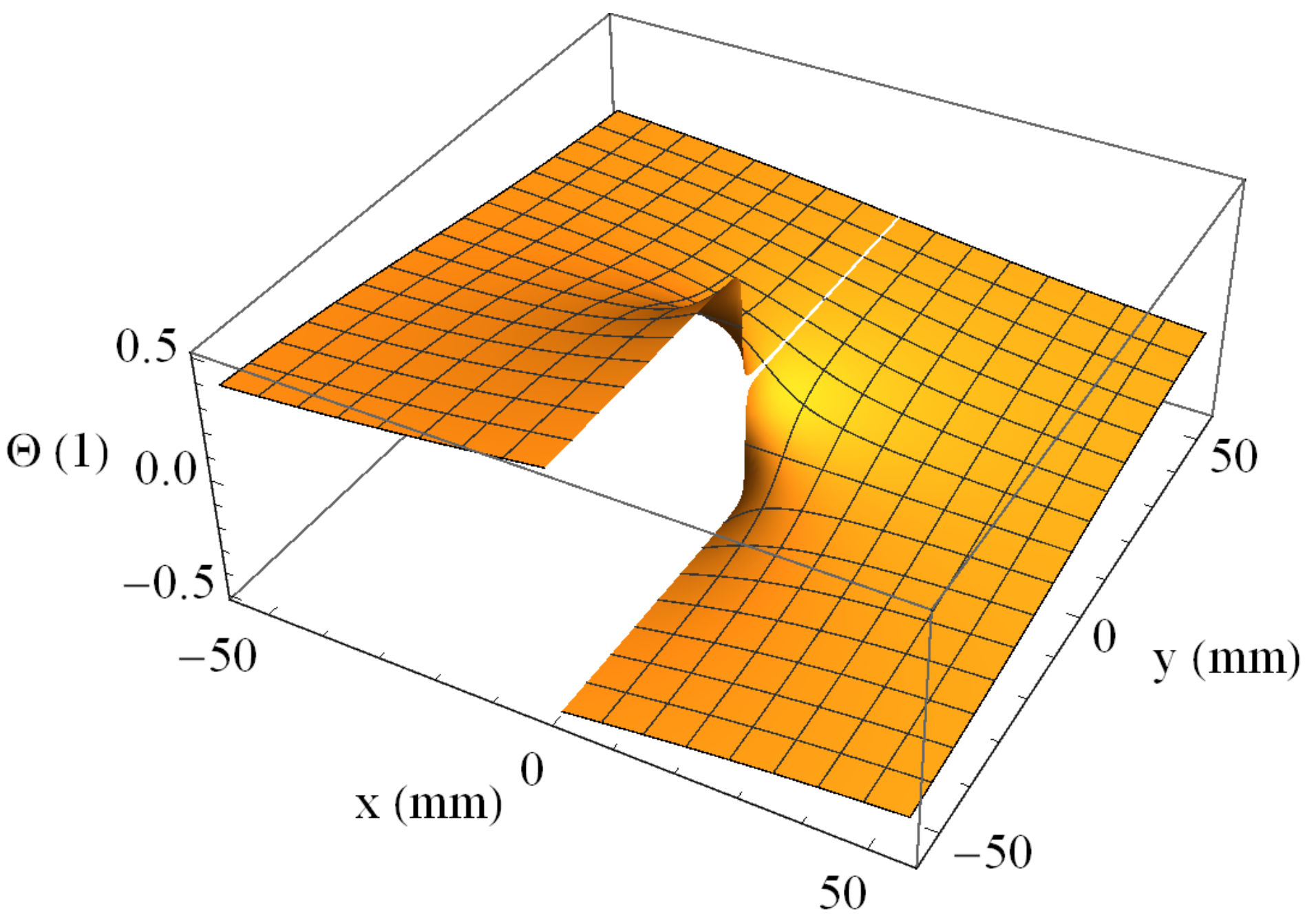
Moreover, to obtain a helical-type spatial phase to the full laser field, the approach was to simulate the reflection of the beam on a “helical” mirror. The mirror would imprint a specific phase distribution upon the beam due to its surface topology, defined by:
where s is the step between the two edges of the helical mirror and is proportional to the cylindrical coordinate , with some modifications to include the full domain:
The function that describes the helical wavefront is depicted in Figure 1.
The reflection on a helical mirror described by Equation (7) would imprint a corresponding phase on each Gausslet:
There is also a shift in the temporal factor of the Gausslet due to the delays caused by the helical mirror. Each individual Gausslet centered initially at and , is modified by the terms containing s and therefore becomes dependent on the spatial positions i and j:
and are the pulse duration and central angular frequency of the m pulselet term in the decomposition. is the speed of light. Please note the difference between the imaginary number and the index i.
3. Results of the Simulations
The propagation code, described previously and detailed in [30], helped to simulate the behavior of the 55 mm Supergaussian laser field, with 25 fs at FL. The full electric field was reconstructed through the superposition of all the spatio-temporal Gausslets.
In the following, several helical cases are presented and discussed: without or with spatio-temporal distortions. Please note that several wavefront distortions were analyzed elsewhere by Ohland and co-authors [31] and will not be discussed here further.
3.1. Ultrashort Laser Fields with Helical Phases
In this subsection, we consider the case of pulses without STC in three configurations: a non-distorted laser field with a helical phase of OAM , at best compression, then with phase jumps corresponding to fractional or higher-order OAM and, finally, with OAM for pulses chirped in time.
Through this preliminary analysis, we intend to present the ideal case and the impact of small helicity and chirp deviations on the overall field distribution, in the absence of the STC.
3.1.1. Helical Mirror with Matched Step–Wavelength
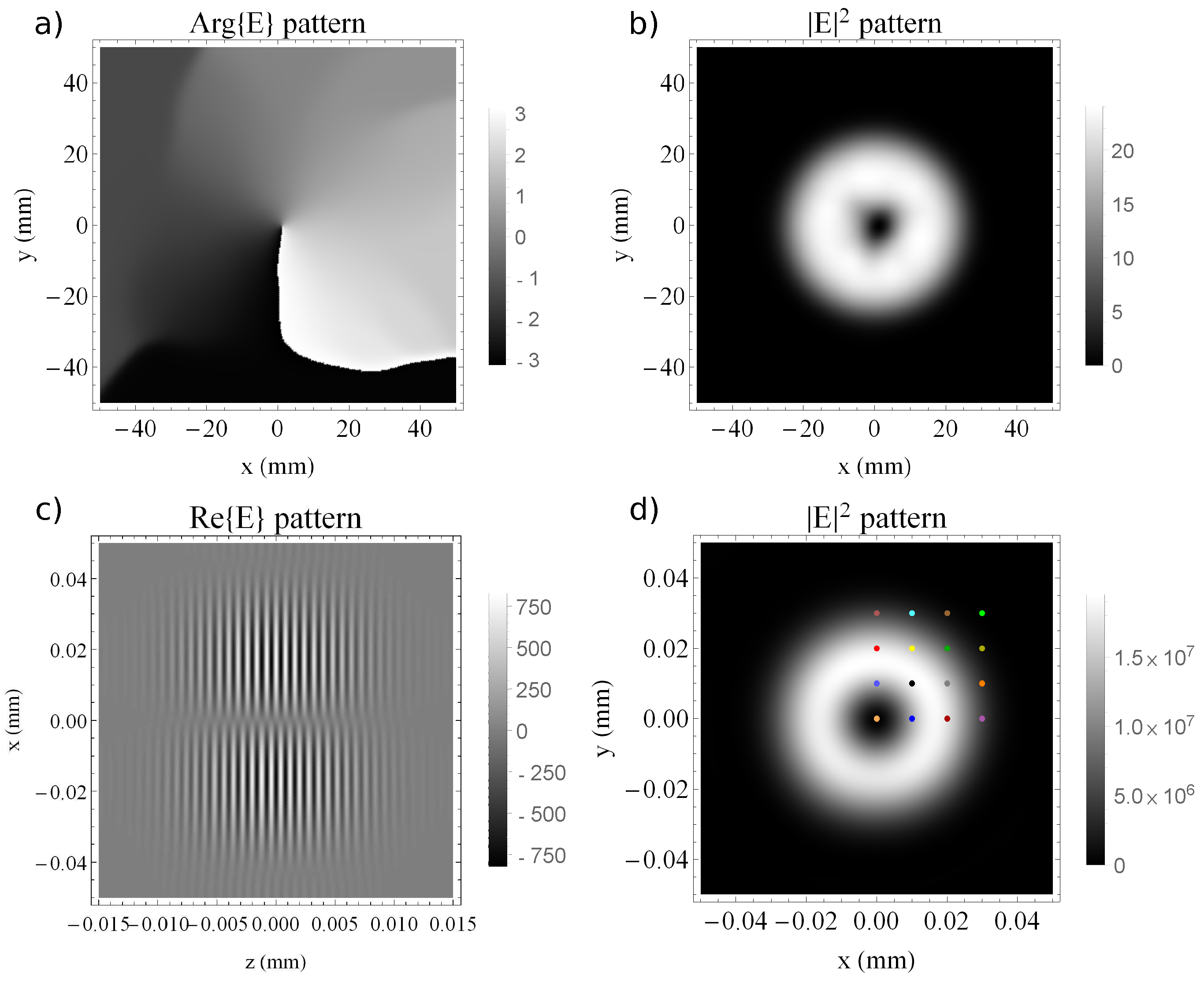
The case of the perfect helical phase at best compression, OAM corresponding to is presented in Figure 2, for the Supergaussian field. The reconstructed wavefront in Figure 2a reproduces the phase jump introduced using Equation (7), corresponding to the theoretical wavefront from Figure 1. The phase values are not relevant on the edges of the plot, because the beam does not cover the full area (the beam size is visible in plot b of Figure 2).
Furthermore, in Figure 2b one can observe the expected “doughnut” shape of the time-integrated irradiance profile associated with the Supergaussian beam, which is visible through the use of detection cameras in the laboratory [34]. The number of Gausslets in the decomposition was 121 (spatial) × 23 (temporal), as previously mentioned.
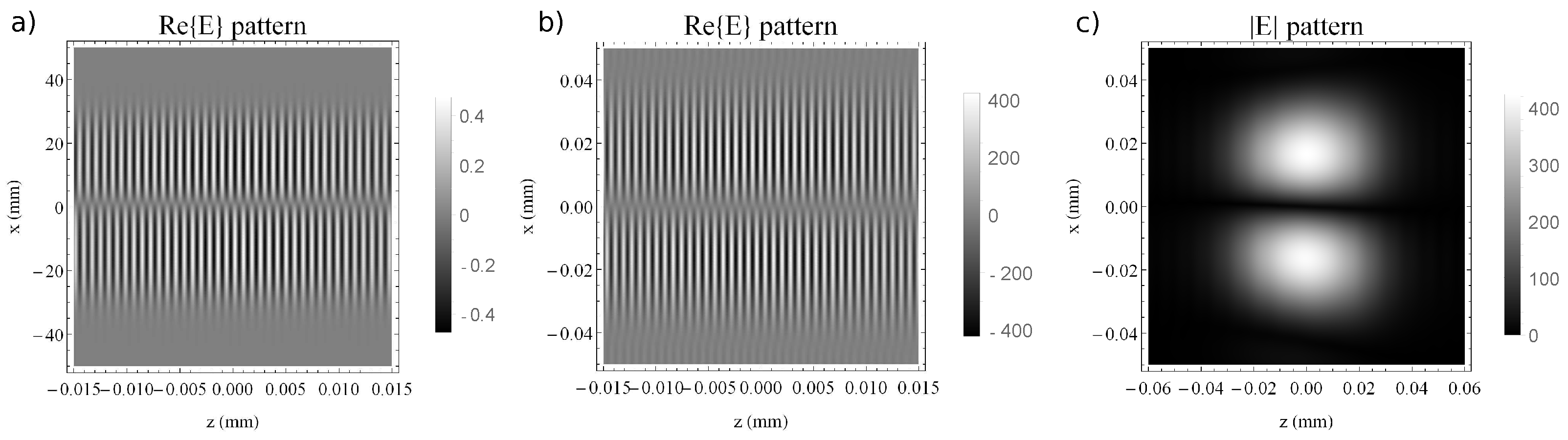
It is also possible to propagate and reconstruct the complete structure of the field in the focal plane, including the carrier modulation, as presented in Figure 2c. The phase shift between the upper and lower lobes in the plane cut is reproduced, as expected, indicating the spiral field structure in the propagation direction z. Moreover, the channel in the middle is preserved after focusing and the doughnut shape is preserved in the focal plane shown in Figure 2d, as pointed out also in [35]. It is well known that the behavior of the focused fields corresponds to the fields propagating in free space at infinity–known as the far field (FF). Therefore, similar behavior must appear at long propagation distances in free space.
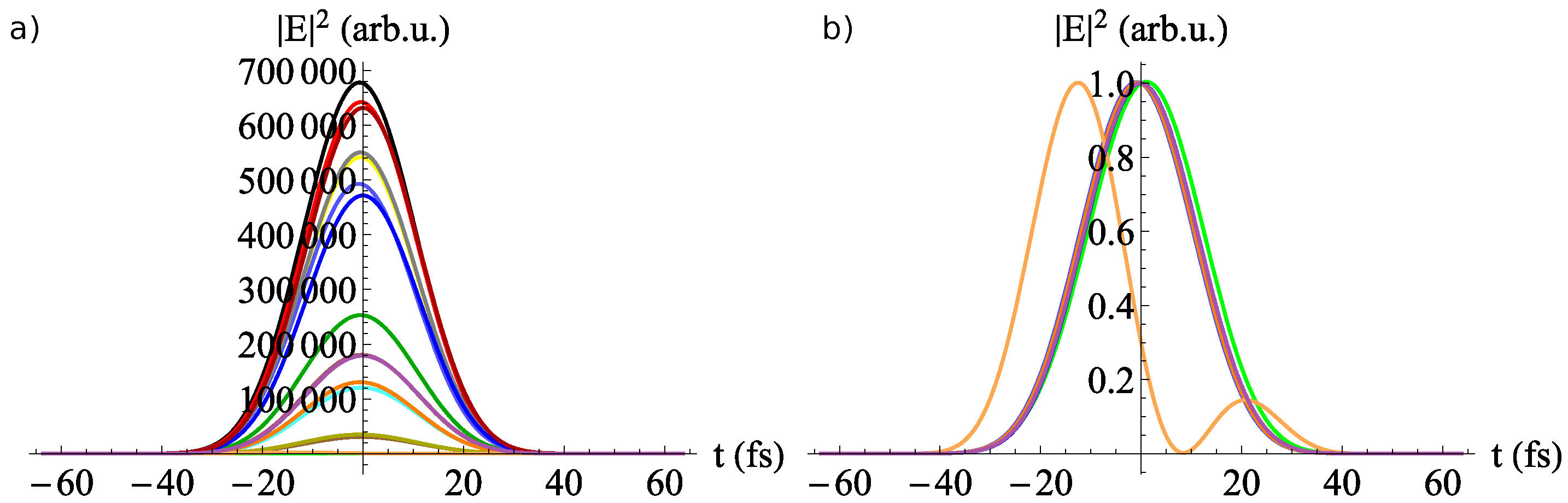
The pulse temporal shape remains Gaussian in different spatial positions from the doughnut profile. The field varies in intensity, as one can see in Figure 3a–where each temporal profile is represented with the color of the corresponding dot from the fluence profile in Figure 2d. Figure 3b was obtained by normalizing the temporal envelopes in Figure 3a in order to prove that the temporal shape envelope remained the same for all the dots. The shape of the light orange curve corresponds to the one in the center of the doughnut and it is not relevant, as its signal was very low (almost zero compared to the others, i.e., 2200 arb.u. at the peak, or % of the largest peak, so it cannot be seen in the non-normalized plot). This is also the case for the light green curve, corresponding to the edge of the beam profile.
3.1.2. Helical Mirror with Different Surface Steps
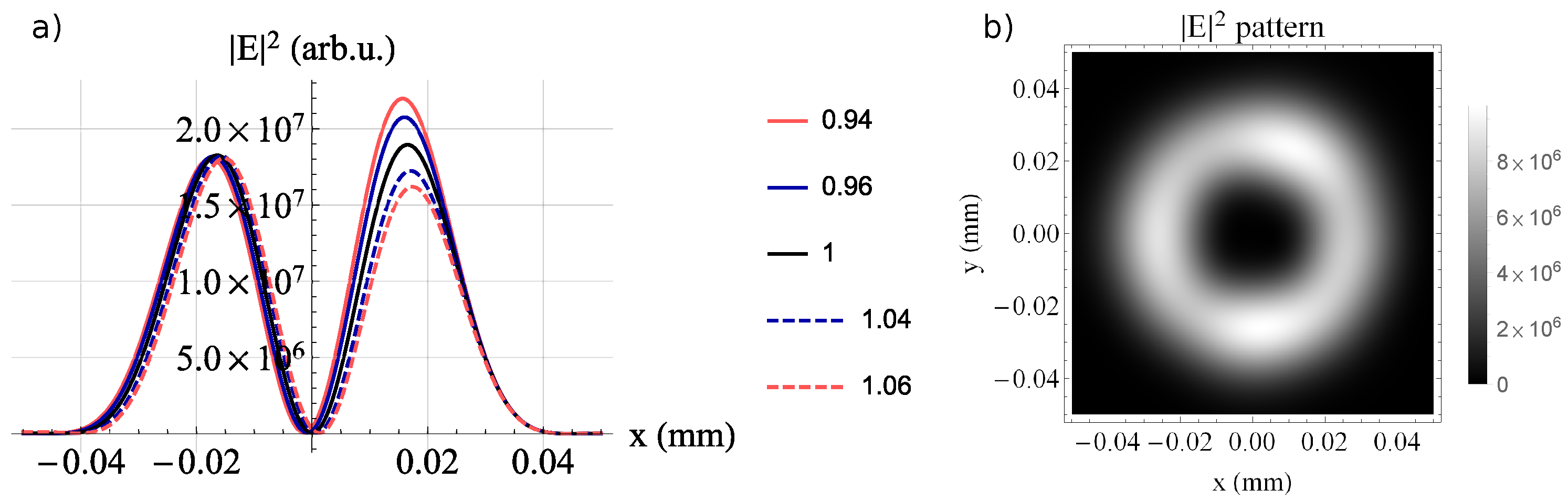
It can be observed sometimes that the doughnut shape is asymmetric, indicated by the fact that one of the lobes is more intense than the other, as in Figure 4a. Simulating the helical laser field introduced above, with different values of the step , showed that variations of a few percentage points in the factor K lead to noticeable lobe amplitude variations.Therefore, not matching the central laser wavelength with the step of the helical mirror causes distortions in the ring shape.
Figure 3.
The temporal profile () of the laser field after being reflected by the helical mirror and focused with an mm mirror. The colors correspond to the positions where the fluence profile is marked in Figure 2d: (a) non-normalized and (b) normalized. The light orange plot corresponds to , where the signal is only an irrelevant, small amount of noise. Normalization was performed so that the maximum of each plot reached 1. The maximum value of the light orange plot appeared close to fs, whereas at the signal dropped.

On the other hand, the higher the factor K, the higher the OAM and therefore the beam size increases, as one can see in Figure 4a,b. As an example, the shape for corresponding to OAM = 2 looks irregular in Figure 4b, this time due to the decomposition of the full beam into a limited number of Gaussian terms (121). The larger the spatial modulations of the beam, the more terms are needed in the decomposition to decrease the reconstruction error. In the following sections, we restrict the analysis to OV with OAM = 1, as this value is the most accessible for practical implementation in high-power laser experiments.
Figure 4.
(a) The fluence profile ( time-integrated) on x, when , of the laser field after being reflected by the helical mirror of and focused with an mm mirror. The K value is given in the legend. (b) The fluence profile ( time-integrated) of the laser field after being reflected by the helical mirror with and focused with an mm mirror.

3.1.3. Chirped Laser Pulse and Helical Spatial Phase
Chirping of the laser field can be achieved by adding dispersion to the FL pulse. Therefore, the spectral amplitude remains the same, but the spectral phase becomes non-flat and the pulse duration increases. In these simulations, the pulse duration was chirped from the pulse width at FL to . The spatial phase of this field also becomes helical after reflection on the helical mirror of step s.
The channel in the center, both in the near field (NF), shown in Figure 5a, and in the focus, shown in Figure 5b,c, is similar to the FL case, with the difference that the pulse duration is four times longer. Furthermore, the field amplitude decreases, according to the energy conservation principle. Figure 5a,b demonstrate that the wavefronts exhibited the helical beam characteristic shift between the upper and the lower lobes, indicating that a spiral pattern (and the doughnut) was also preserved. The plots in Figure 5a,b are represented at a smaller scale for z, in order to resolve the wavefront oscillations.
3.2. Laser Fields with Helical Phases and Spatio-Temporal Distortions
In order to model the STC of the initial laser field, specific variations in the parameters of the Gausslets were considered. The helical phase was introduced to these STC fields. The results of the simulations are presented and commented upon in the following.
3.2.1. Spatial Chirp
Spatial chirp (SPC) is the linear variation of the spatial properties for each frequency component in the spectrum: [30,36,37]. Here, we considered the initial Gaussian to be 25 fs FL at nm, with the temporal pulse shape measured in the spatial center of the beam, at . When there is SPC in the field, then the central frequency of the wave will change according to the SPC variation, meaning that the spectrum will be a different one at each position x: , where is the central frequency of the m pulselet in the decomposition. Simulations were performed with SPC on the x axis with the value of mm/PHz, for a consistent comparison with the non-helical case in [30].
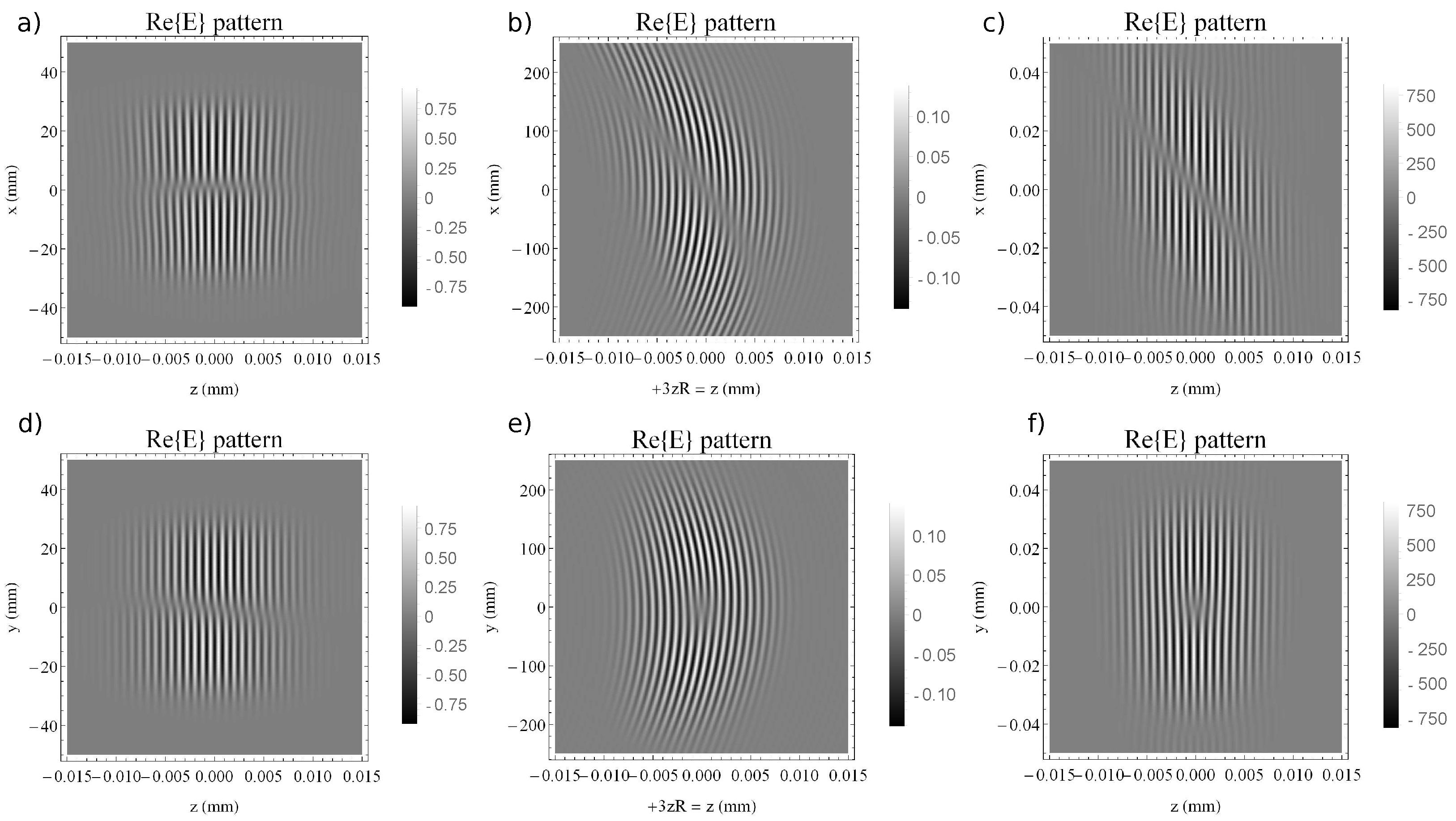
Figure 6 presents the NF, FF and focused distributions of the field in the plane (upper row) and in the plane (lower row). Figure 6a,d correspond to the NF profiles on and , respectively. In addition to the characteristic fan of the SPC and the channel that appears due to the helicity, a slightly tilted channel in the plane can be distinguished. In Figure 6b,e the wavefront is still slightly curved, as the divergence of the beams at is not perfectly zero.
As previously mentioned, the behavior of the focused fields corresponds to the fields in the FF. The reconstructed focused field is presented in Figure 6c,f. The wavefront curvature vanishes here, as expected. A gap is apparent on the longitudinal z axis in both FF and focus profiles, which can be associated with the temporal shape, in the profiles. Therefore, there is a spatio-temporal vortex that appears. A comparable behavior of the field was described in [38,39], where the production of spatio-temporal optical vortices was investigated in simulations and in experiments.
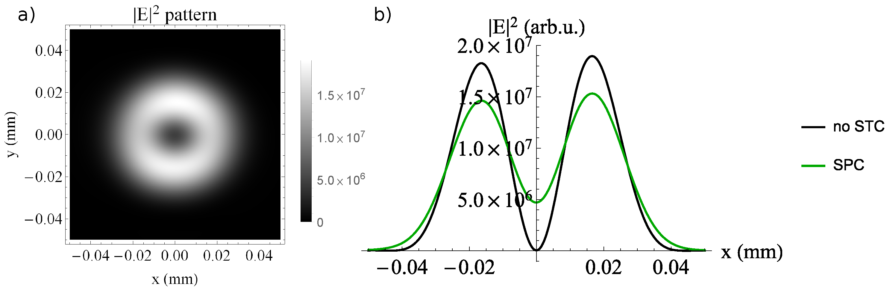
Figure 7 presents the time-integrated profile in the focus area, that corresponds in practice to an image recorded with a camera sensor. The field in the central part of the doughnut is not going down to zero anymore, as in the case of non-distorted laser pulses. The SPC from the NF generates a tilt in the pulse front in the focus [30] and the time-integrated (fluence) profile has a positive value in the center, as shown in Figure 7b. This can be interpreted as a distinctive signature of the presence of SPC in the helical pulse and it appears at relatively small residual SPC values. This sensitivity can be turned into an advantage through the design of a camera-based device that includes a focusing element and a helical phase plate that can detect such small SPC.
3.2.2. Angular Dispersion
The angular dispersion, or angular chirp (AGC), is the variation of the angle at which a specific laser field propagates with its frequency, . For example, it can be generated when different frequency components in the spectrum are diffracted at different angles by a grating and, therefore, each of the spectral components will be tilted with different angles.
The implementation of the AGC in the code used here was performed by tilting each Gausslet with a specific propagation angle (around the axis ). The linear correspondence with each m component in the temporal/spectral decomposition was as in [30]: and the AGC value was mrad/PHz on the x axis, generated, for example, by an approximately 125 µrad grating misalignment in a double-grating compressor.
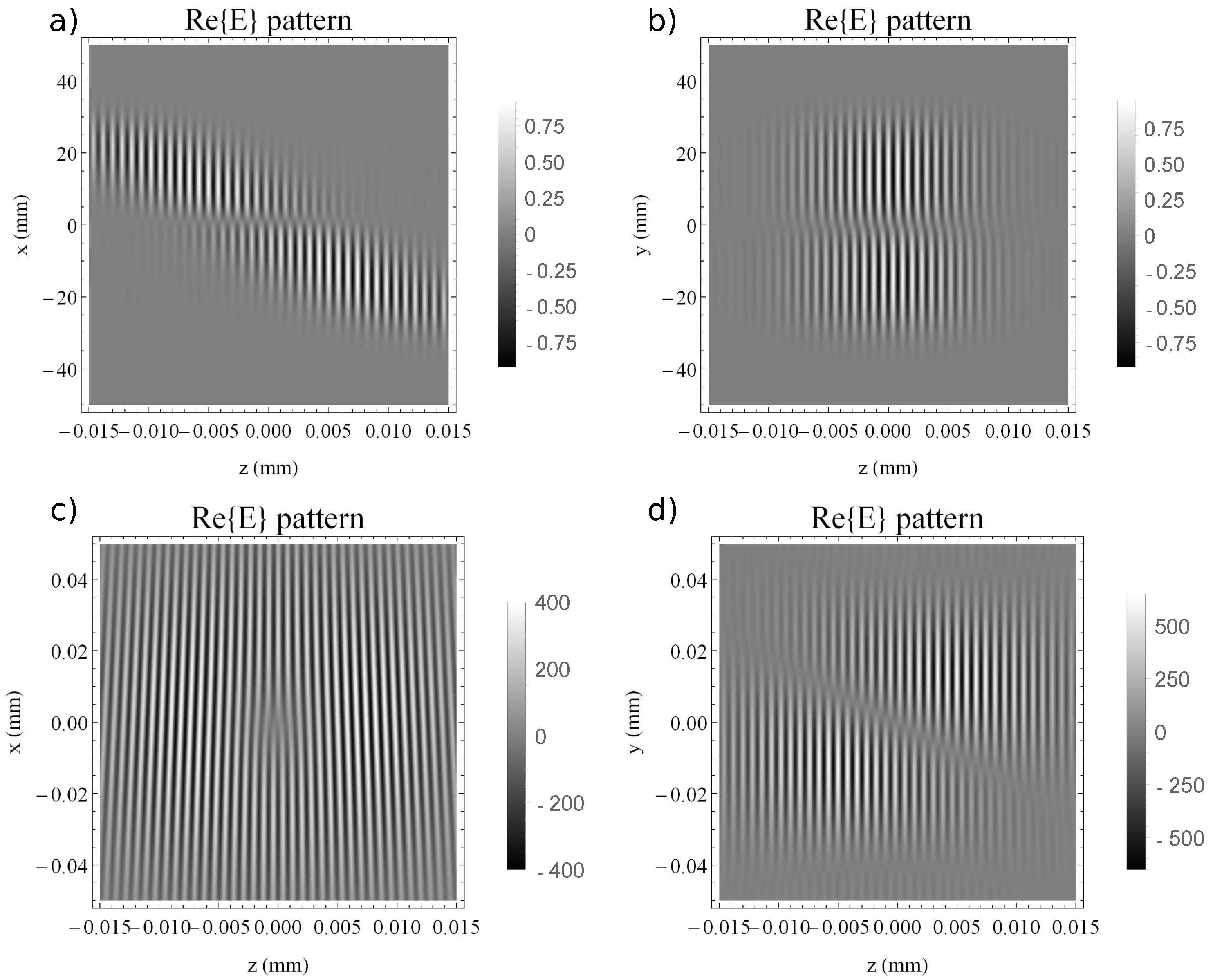
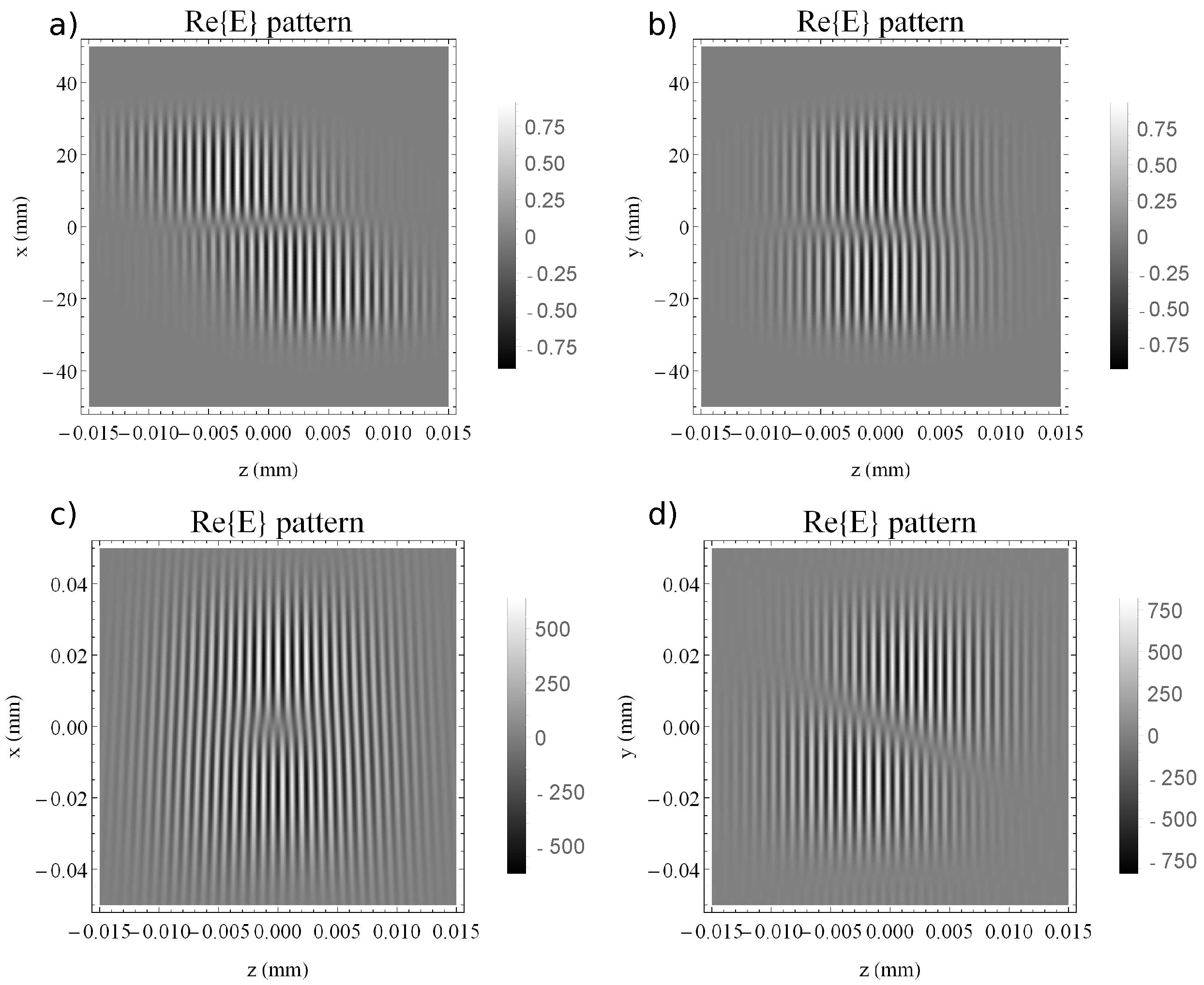
In Figure 8a,b one can observe the NF pattern in the and in the planes, with the specific central singularity of the helical phase. The pulse front tilt associated with the AGC is present, as expected, in the profile. The focused field is depicted in Figure 8c,d in the focal region. The expected spatial chirp is present and can be observed as a variable front tilt in the plane, in Figure 8c, along with a diagonal phase dislocation in the longitudinal profile on from Figure 8d.
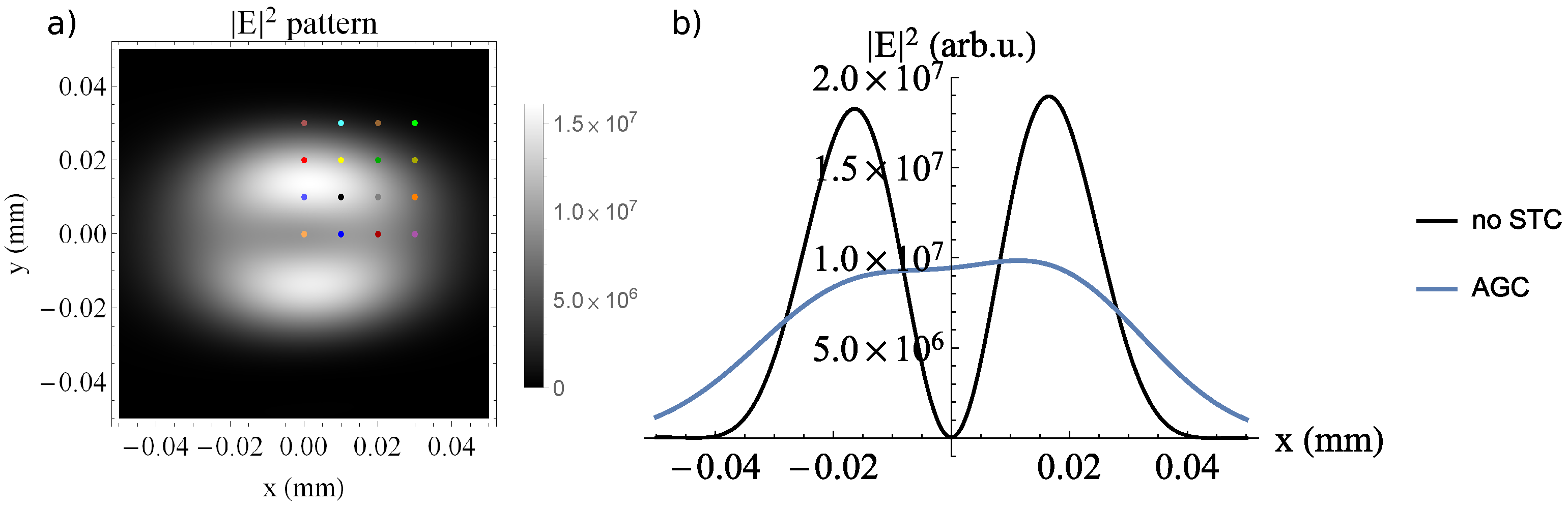
Changing the perspective, the time-integrated profile is depicted in Figure 9a. The doughnut tends to form two symmetric lobes with respect to the axis. Furthermore, the field in the central hole does not drop to zero, as shown in the time-integrated profile at , Figure 9b. This indicates, similarly to the SPC case, a signature of the high sensitivity of the intensity profile to the presence of AGC in the helical phase pulses.
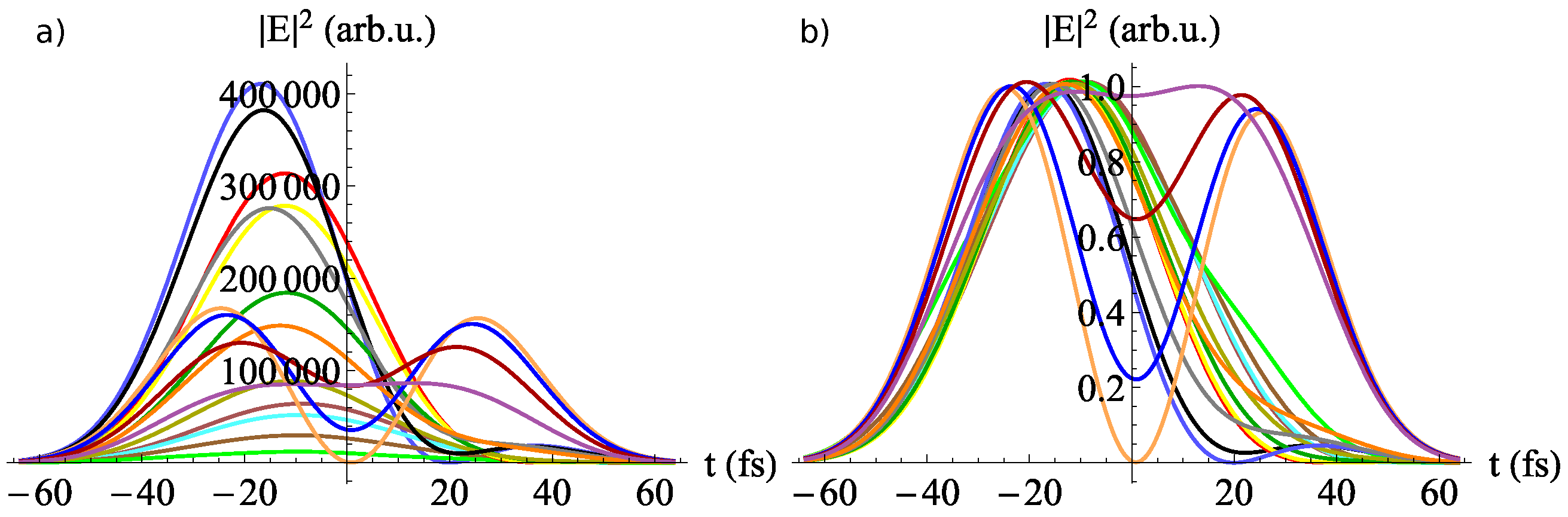
Furthermore, the temporal behavior of the pulse was analyzed in the focus, in Figure 10. The temporal evolution of the irradiance is depicted in the non-normalized (inset a) and normalized cases (inset b). One striking difference with respect to the ideal helical case depicted in Figure 3 is the presence of two temporal lobes. They can be symmetric or unbalanced in the field envelope. Further, the position of the maxima of the lobes shifts in time, whereas the lobe width varies, indicating the variable local pulse duration.
Several temporal envelopes can be observed in Figure 10, corresponding to horizontal cuts in the field representation of focused pulses with AGC from Figure 8c,d. This occurred due to the fact that there was a linear mapping between the propagation axis z and the temporal coordinate t. Hence, the presence of the two temporal lobes indicates the existence of the phase jump in the plane, as shown in Figure 8c, whereas the shifts of the lobes and the asymmetry correspond to the tilted phase dislocation channel depicted in Figure 8d in the plane.
3.2.3. Pulse Front Tilt
In lasers with STC it can happen that the wavefront and the pulse front do not coincide. When there is a linear coupling between the temporal and spatial coordinates in the formula of the laser field, this factor is known as pulse front tilt (PFT): [36].
In the current work, PFT was implemented as in [30] such that the central time coordinate (the average of each temporal Gaussian m) is shifted proportionally to the spatial position : . A value of fs/mm was used for consistent comparison with the plots from [30].
Figure 11a,b depict the detailed field distribution in the NF in the and planes. These results look similar to the ones obtained in the case of AGC, presented in Figure 8. This is due to the fact that the PFT is equivalent with the AGC (in the absence of frequency chirp) [36,37]). The same qualitative behavior is also observed after the propagation of the helical PFT pulses to the focal plane, as shown in Figure 11c,d in the and planes.
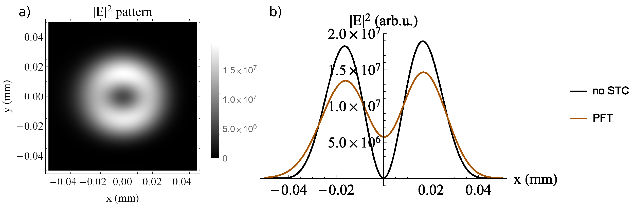
In Figure 12, the time integrated profile is depicted for the helical pulse with fs/mm, after propagation to the focal plane. Furthermore, a similar qualitative behavior is also observed here with respect to the AGC case. The depth of central hole in the beam profile is reduced in the presence of the PFT, as shown in Figure 12b, in comparison with the ideal case where no STC is present in the helical pulse.
4. Discussion
In this study, the four-dimensional propagation of ultrashort optical vortices was simulated, for the first time to our knowledge, using a Gaussian decomposition code. The expected behavior in the case of non-distorted ultrashort optical vortices was obtained. Stretching and compressing the temporal shape proved that the phase displacements were maintained so that the beam profile remained of the doughnut type both in the NF and focus regions.
However, when residual STC was present in the laser field of OV, the behavior of the singularity was modified. One effect that could be easily observed in the experiments was that the central deep areain the beam profile started to wash out. As shown in Figure 7 for the case of SPC, in Figure 9 for AGC and in Figure 12 for PFT initial distortions, the amplitude of the signal in the center became significant and this can be clearly measured with a video camera. Small values of these STC distortions were enough to provide this effect, indicating a high sensitivity of the central deep amplitude of the doughnut shape.
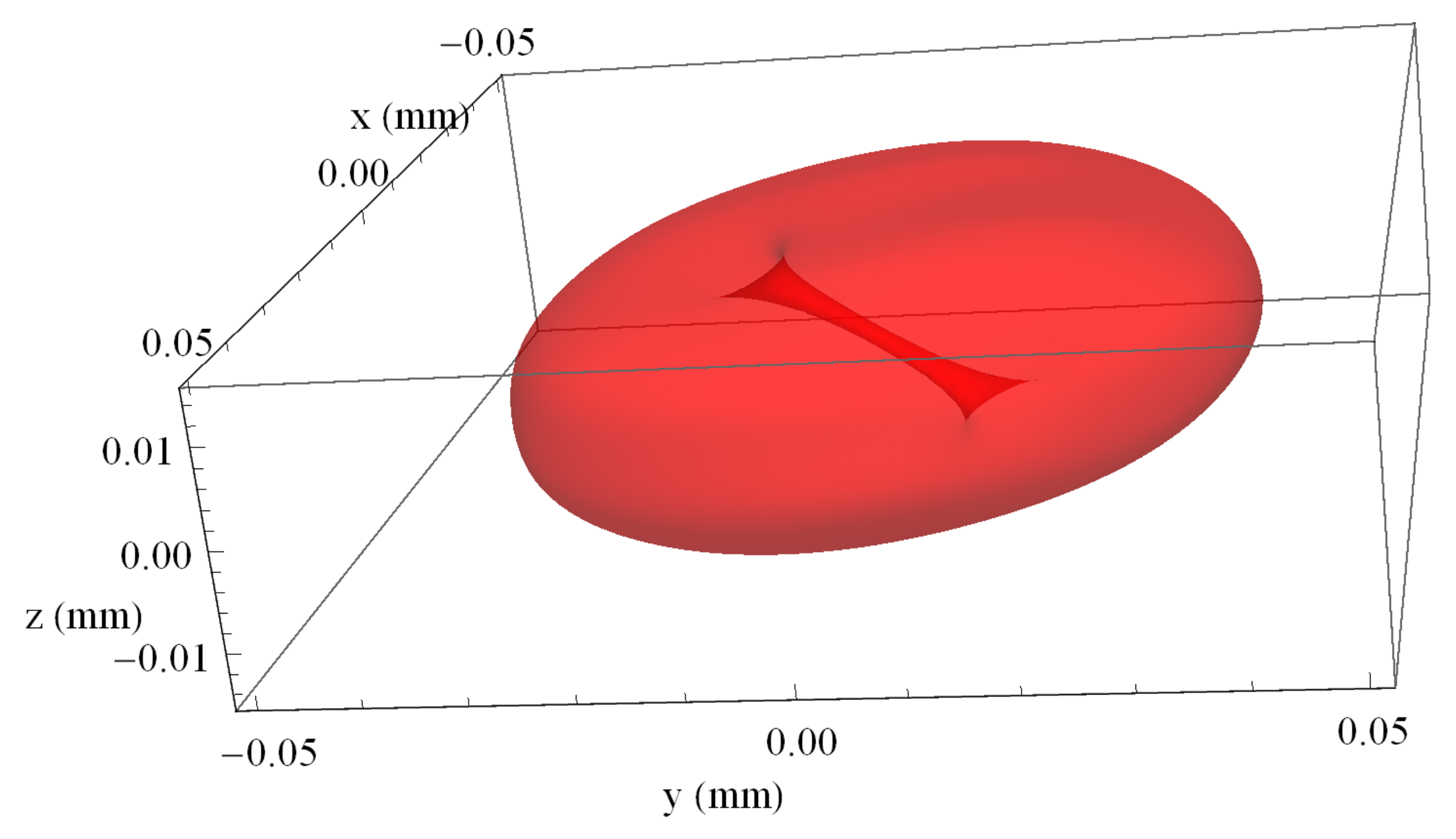
The presence of the singularity was clearly observed in the detailed cuts in the focus areas of the SPC-, AGC- and PFT-distorted OV pulses. In order to illustrate this effect specifically for the PFT case, Figure 13 presents, at scale, a three-dimensional region plot of the pulse corresponding to the two-dimensional cuts from Figure 11c,d. It indicates that the singularity was rotated but it did not disappear. The wash out effect in the beam profile was the consequence of this rotation of the singularity orientation in the pulse along the propagation. The same rotation was responsible for the wash-out of the hole in the beam profile in the case of SPC and AGC. This rotation, even in the presence of small STC, provides additional challenges in the implementation of experiments.
Moreover, as discussed in [30], the SPC in NF generates PFT in the focus. AGC and PFT are equivalent in the absence of temporal chirp, and both of them in NF generate SPC in the focus. This behavior can also be distinguished for optical vortexes, as the field distribution is influenced by both helicity and STC. The effect of generating a specific vortex pattern in time as well, aside from the spatial effect, is an outcome of these processes [39].
Consequently, the high sensitivity of the helical pulses to the residual STCs might provide a simple path towards practical implementation of spatio-temporal optical vortices [39,40] in CPA laser systems by simply misaligning the optical stretcher or the compressor. This comes with the more subtle effects of local double pulses in the temporal profile, as shown in Figure 10.
Experiments that use helical beams—such as proton acceleration [23,41] indicating the enhanced behavior of the accelerated particles when using doughnut beams—need to take into account the effects of the STCs in the implementation and metrology phase, in order to produce the expected results. There have been many proposals of experiments using ultrashort helical pulses, e.g., in the production of gamma rays [42] and positron production [43], attosecond electron bunches with OAM [44] and relativistic electron mirrors [45], and in all these, the laser intensity distribution on the target must be optimized through systematic measurements of the STC of the vortex-free laser field.
5. Conclusions
The introduction of ultrashort laser pulses and of the CPA technique during the last quarter of the 20th century raised the need for an in-depth understanding of STC in the propagation of laser fields. This was accomplished through the development of complex metrology techniques, and also through the software development of four-dimensional propagation codes for broadband ultrashort laser pulses, such as the one used here.
In a complimentary fashion, pulse shaping techniques that implement deformable mirrors, spatial light modulators or specific optical components have enabled advances in spatially-tailored laser pulses. In particular, OVs were proposed to be used in conjunction with ultra-intense pulses from CPA laser systems in order to enhance the desired light–matter interaction effects in processes such as electron and proton acceleration. Although the impact of wavefront distortions on OVs has been reported in [31], one type of spatio-temporal distortions had not been investigated to date, to our knowledge.
A Gaussian decomposition code was used to investigate the joint presence of the OV and STC in ultrashort laser pulses and their effects in the focal plane, as required in several proposed experiments. We took as a reference the HPLS laser parameters available at ELI-NP, as these are also common to several petawatt class facilities: a Supergaussian spatial profile and a 25 fs pulse duration at a 800 nm central wavelength.
The simulations showed the evolution of the OV phase dislocation in space and time. We have also pointed out that the sensitivity of the far field to the residual STCs can help in the design of new metrology devices that provide quantitative evaluations of the STC. The results of this study will help researchers to understand better the effects of residual STCs, enabling the advanced design and implementation of future extreme light experiments with complex OV pulses.
Author Contributions
Conceptualization, D.U. and A.-M.T.; methodology, A.-M.T. and D.U.; software, A.-M.T.; validation, A.-M.T., V.I. and D.U.; formal analysis, A.-M.T.; investigation, A.-M.T. and V.I.; writing—original draft preparation, A.-M.T., V.I. and D.U.; writing—review and editing, A.-M.T., V.I. and D.U.; visualization, A.-M.T.; supervision, D.U.; project administration, D.U.; funding acquisition, D.U. All authors have read and agreed to the published version of the manuscript.
Funding
This research was funded by the Institute of Atomic Physics, Romania, grant number ELI-RO 16/2020 SBUF and by the Ministry of Education and Research, CNCS-UEFISCDI (project no. PN-IIIP4-ID-PCCF-2016–0164), within PNCDI III. The authors are thankful for the financial support from the Nuclei Project (PN 19060105). The APC was funded by PN-IIIP4-ID-PCCF-2016–0164.
Institutional Review Board Statement
Not applicable.
Informed Consent Statement
Not applicable.
Data Availability Statement
Data available on request.
Acknowledgments
The authors would like to express their appreciation to Takahisa Jitsuno, Ioan Dancus, Dan Stutman, Mihail Cernaianu, Petru Ghenuche and Dan Gh. Matei from the Extreme Light Infrastructure Nuclear Physics (ELI-NP) facility of the National Institute of Physics and Nuclear Engineering Horia Hulubei (IFIN-HH) for supporting discussions and advice. This paper is based on a presentation prepared for the ’1st International Conference–Advances in 3OM: Opto-Mechatronics, Opto-Mechanics, and Optical Metrology’, 13–16 December 2021, Timisoara, Romania.
Conflicts of Interest
The authors declare no conflict of interest.
Abbreviations
The following abbreviations are used in this manuscript:
| AGC | Angular chirp |
| BPM | Beam propagation method |
| CPA | Chirped pulse amplification |
| ELI-NP | Extreme Light Infrastructure–Nuclear Physics |
| FDTD | Finite-difference time domain |
| FF | Far field |
| FL | Fourier limit |
| HPLS | High-power laser system |
| Laguerre-Gaussian | |
| NF | Near field |
| OAM | Orbital angular momentum |
| OPCPA | Optical parametric chirped pulse amplification |
| OV | Optical vortex |
| PFT | Pulse front tilt |
| PW | Petawatt |
| SPC | Spatial chirp |
| STC | Spatio-temporal couplings |
References
- Strickland, D.; Mourou, G. Compression of amplified chirped optical pulses. Opt. Commun. 1985, 56, 219–221. [Google Scholar] [CrossRef]
- Dubietis, A.; Jonušauskas, G.; Piskarskas, A. Powerful femtosecond pulse generation by chirped and stretched pulse parametric amplification in BBO crystal. Opt. Commun. 1992, 88, 437–440. [Google Scholar] [CrossRef]
- Lureau, F.; Matras, G.; Chalus, O.; Derycke, C.; Morbieu, T.; Radier, C.; Casagrande, O.; Laux, S.; Ricaud, S.; Rey, G.; et al. High-energy hybrid femtosecond laser system demonstrating 2 × 10 PW capability. High Power Laser Sci. Eng. 2020, 8, E43. [Google Scholar] [CrossRef]
- Nye, J.F.; Berry, M.V. Dislocations in wave trains. Proc. R. Soc. London A Math. Phys. Sci. 1974, 336, 165–190. [Google Scholar] [CrossRef]
- Coullet, P.; Gil, L.; Rocca, F. Optical vortices. Opt. Commun. 1989, 73, 403–408. [Google Scholar] [CrossRef]
- Bazhenov, V.; Vasnetsov, M.; Soskin, M. Laser-Beams with Screw Dislocations in Their Wave-Fronts. JETP Lett. 1990, 52, 429–431. [Google Scholar]
- Beijersbergen, M.; Allen, L.; van der Veen, H.; Woerdman, J. Astigmatic laser mode converters and transfer of orbital angular momentum. Opt. Commun. 1993, 96, 123–132. [Google Scholar] [CrossRef]
- Allen, L.; Beijersbergen, M.W.; Spreeuw, R.J.C.; Woerdman, J.P. Orbital angular momentum of light and the transformation of Laguerre-Gaussian laser modes. Phys. Rev. A 1992, 45, 8185–8189. [Google Scholar] [CrossRef]
- Grier, D.G. A revolution in optical manipulation. Nature 2003, 424, 810–816. [Google Scholar] [CrossRef]
- Mair, A.; Vaziri, A.; Weihs, G.; Zeilinger, A. Entanglement of the orbital angular momentum states of photons. Nature 2001, 412, 313–316. [Google Scholar] [CrossRef] [Green Version]
- Molina-Terriza, G.; Torres, J.P.; Torner, L. Twisted photons. Nat. Phys. 2007, 3, 305–310. [Google Scholar] [CrossRef]
- Devlin, R.C.; Ambrosio, A.; Rubin, N.A.; Mueller, J.P.B.; Capasso, F. Arbitrary spin-to–orbital angular momentum conversion of light. Science 2017, 358, 896–901. [Google Scholar] [CrossRef] [PubMed] [Green Version]
- Stav, T.; Faerman, A.; Maguid, E.; Oren, D.; Kleiner, V.; Hasman, E.; Segev, M. Quantum entanglement of the spin and orbital angular momentum of photons using metamaterials. Science 2018, 361, 1101–1104. [Google Scholar] [CrossRef] [PubMed]
- Gong, M. Recent Advances on Tunable Vortex Beam Devices for Biomedical Applications. Biomed. J. Sci. Tech. Res. 2018, 9, 5. [Google Scholar] [CrossRef]
- Fuerhapter, S.; Jesacher, A.; Bernet, S.; Ritsch-Marte, M. Spiral phase contrast imaging in microscopy. Opt. Express 2005, 13, 689–694. [Google Scholar] [CrossRef] [Green Version]
- Tamburini, F.; Anzolin, G.; Umbriaco, G.; Bianchini, A.; Barbieri, C. Overcoming the Rayleigh Criterion Limit with Optical Vortices. Phys. Rev. Lett. 2006, 97, 163903. [Google Scholar] [CrossRef] [Green Version]
- Hell, S.W. Microscopy and its focal switch. Nat. Methods 2008, 6, 24–32. [Google Scholar] [CrossRef] [Green Version]
- Barreiro, J.T.; Wei, T.C.; Kwiat, P.G. Beating the channel capacity limit for linear photonic superdense coding. Nat. Phys. 2008, 4, 282–286. [Google Scholar] [CrossRef] [Green Version]
- Lee, J.C.T.; Alexander, S.J.; Kevan, S.D.; Roy, S.; McMorran, B.J. Laguerre–Gauss and Hermite–Gauss soft X-ray states generated using diffractive optics. Nat. Photonics 2019, 13, 205–209. [Google Scholar] [CrossRef] [Green Version]
- De las Heras, A.; Pandey, A.K.; Román, J.S.; Serrano, J.; Baynard, E.; Dovillaire, G.; Pittman, M.; Durfee, C.G.; Plaja, L.; Kazamias, S.; et al. Extreme-ultraviolet vector-vortex beams from high harmonic generation. Optica 2022, 9, 71–79. [Google Scholar] [CrossRef]
- Allen, L.; Padgett, M.; Babiker, M. The Orbital Angular Momentum of Light. In Progress in Optics; Elsevier: Amsterdam, The Netherlands, 1999; pp. 291–372. [Google Scholar] [CrossRef]
- Nuter, R.; Korneev, P.; Dmitriev, E.; Thiele, I.; Tikhonchuk, V.T. Gain of electron orbital angular momentum in a direct laser acceleration process. Phys. Rev. E 2020, 101, 053202. [Google Scholar] [CrossRef] [PubMed]
- Brabetz, C.; Busold, S.; Cowan, T.; Deppert, O.; Jahn, D.; Kester, O.; Roth, M.; Schumacher, D.; Bagnoud, V. Laser-driven ion acceleration with hollow laser beams. Phys. Plasmas 2015, 22, 013105. [Google Scholar] [CrossRef]
- Dennis, M.R.; O’Holleran, K.; Padgett, M.J. Chapter 5 Singular Optics: Optical Vortices and Polarization Singularities. In Progress in Optics; Elsevier: Amsterdam, The Netherlands, 2009; pp. 293–363. [Google Scholar] [CrossRef]
- Pariente, G.; Gallet, V.; Borot, A.; Gobert, O.; Quéré, F. Space–time characterization of ultra-intense femtosecond laser beams. Nat. Photonics 2016, 10, 547–553. [Google Scholar] [CrossRef]
- Dorrer, C. Spatiotemporal Metrology of Broadband Optical Pulses. IEEE J. Sel. Top. Quantum Electron. 2019, 25, 1–16. [Google Scholar] [CrossRef]
- Greynolds, A.W. Propagation Of Generally Astigmatic Gaussian Beams Along Skew Ray Paths. In Proceedings of the Diffraction Phenomena in Optical Engineering Applications; Byrne, D.M., Harvey, J.E., Eds.; International Society for Optics and Photonics, SPIE: Bellingham, WA, USA, 1986; Volume 0560, pp. 33–51. [Google Scholar] [CrossRef]
- Harvey, J.E.; Irvin, R.G.; Pfisterer, R.N. Modeling physical optics phenomena by complex ray tracing. Opt. Eng. 2015, 54, 035105. [Google Scholar] [CrossRef] [Green Version]
- Worku, N.G.; Gross, H. Gaussian pulsed beam decomposition for propagation of ultrashort pulses through optical systems. J. Opt. Soc. Am. A 2020, 37, 98–107. [Google Scholar] [CrossRef]
- Talposi, A.M.; Ursescu, D. Propagation of ultrashort laser fields with spatiotemporal couplings using Gabor’s Gaussian complex decomposition. J. Opt. Soc. Am. A 2022, 39, 267–278. [Google Scholar] [CrossRef]
- Ohland, J.B.; Eisenbarth, U.; Roth, M.; Bagnoud, V. A study on the effects and visibility of low-order aberrations on laser beams with orbital angular momentum. Appl. Phys. B 2019, 125, 202. [Google Scholar] [CrossRef] [Green Version]
- Wolfram Research. NonlinearModelFit, Wolfram Language Function. 2008. Available online: https://reference.wolfram.com (accessed on 30 September 2021).
- Siegman, A. Lasers; University Science Books: Sausalito, CA, USA, 1986; Chapter 17. [Google Scholar]
- Serna, J.; Encinas-Sanz, F.; Nemes, G. Complete spatial characterization of a pulsed doughnut-type beam by use of spherical optics and a cylindrical lens. J. Opt. Soc. Am. A 2001, 18, 1726–1733. [Google Scholar] [CrossRef]
- Zhou, G.; Cai, Y.; Dai, C.Q. Hollow vortex Gaussian beams. Sci. China Phys. Mech. Astron. 2013, 56, 896–903. [Google Scholar] [CrossRef]
- Akturk, S.; Gu, X.; Gabolde, P.; Trebino, R. The general theory of first-order spatio-temporal distortions of Gaussian pulses and beams. Opt. Express 2005, 13, 8642–8661. [Google Scholar] [CrossRef] [PubMed]
- Akturk, S.; Gu, X.; Zeek, E.; Trebino, R. Pulse-front tilt caused by spatial and temporal chirp. Opt. Express 2004, 12, 4399–4410. [Google Scholar] [CrossRef] [PubMed]
- Sukhorukov, A.P.; Yangirova, V.V. Spatio-temporal vortices: Properties, generation and recording. In Proceedings of the Nonlinear Optics Applications; Karpierz, M.A., Boardman, A.D., Stegeman, G.I., Eds.; International Society for Optics and Photonics, SPIE: Bellingham, WA, USA, 2005; Volume 5949, pp. 35–43. [Google Scholar] [CrossRef]
- Hancock, S.W.; Zahedpour, S.; Goffin, A.; Milchberg, H.M. Free-space propagation of spatiotemporal optical vortices. Optica 2019, 6, 1547. [Google Scholar] [CrossRef]
- Chong, A.; Wan, C.; Chen, J.; Zhan, Q. Generation of spatiotemporal optical vortices with controllable transverse orbital angular momentum. Nat. Photonics 2020, 14, 350–354. [Google Scholar] [CrossRef]
- Wang, W.; Jiang, C.; Dong, H.; Lu, X.; Li, J.; Xu, R.; Sun, Y.; Yu, L.; Guo, Z.; Liang, X.; et al. Hollow plasma acceleration driven by a relativistic reflected hollow laser. Phys. Rev. Lett. 2020, 125, 034801. [Google Scholar] [CrossRef]
- Zhang, H.; Zhao, J.; Hu, Y.; Li, Q.; Lu, Y.; Cao, Y.; Zou, D.; Sheng, Z.; Pegoraro, F.; McKenna, P.; et al. Efficient bright γ-ray vortex emission from a laser-illuminated light-fan-in-channel target. High Power Laser Sci. Eng. 2021, 9, 1–24. [Google Scholar] [CrossRef]
- Zhao, J.; Hu, Y.T.; Lu, Y.; Zhang, H.; Hu, L.X.; Zhu, X.L.; Sheng, Z.M.; Turcu, I.C.E.; Pukhov, A.; Shao, F.Q.; et al. All-optical quasi-monoenergetic GeV positron bunch generation by twisted laser fields. Commun. Phys. 2022, 5, 15. [Google Scholar] [CrossRef]
- Hu, L.X.; Yu, T.P.; Sheng, Z.M.; Vieira, J.; Zou, D.B.; Yin, Y.; McKenna, P.; Shao, F.Q. Attosecond electron bunches from a nanofiber driven by Laguerre-Gaussian laser pulses. Sci. Rep. 2018, 8, 7282. [Google Scholar] [CrossRef] [Green Version]
- Hu, L.X.; Yu, T.P.; Li, H.Z.; Yin, Y.; McKenna, P.; Shao, F.Q. Dense relativistic electron mirrors from a Laguerre-Gaussian laser-irradiated micro-droplet. Opt. Lett. 2018, 43, 2615. [Google Scholar] [CrossRef]
Figure 1.
The variation of in Equation (8) with the spatial coordinates x and y, represents the topology of the helical mirror.
Figure 1.
The variation of in Equation (8) with the spatial coordinates x and y, represents the topology of the helical mirror.

Figure 2.
(a) The phase profile of the laser field after being reflected by the helical mirror, at . (b) The fluence profile ( time-integrated) of the laser field after being reflected by the helical mirror, at . (c) The field profile () on of the laser field after being reflected by the helical mirror and focused with an mm mirror. (d) The fluence profile ( time-integrated) of the laser field after being reflected by the helical mirror and focused with an mm mirror. The dots are marking the positions where the temporal profiles are plotted in Figure 3, with the corresponding color.

Figure 5.
The field profile ( on at and ) of the chirped laser, with duration after being reflected by the helical mirror (a) in the NF and (b) in the focal region of an mm mirror (the back focal plane is considered in for simplicity). (c) The corresponding amplitude profile ( on at and ) for the focused field shown in plot (b).

Figure 6.
The electric field profile () of a laser field with mm/PHz, after being reflected by the helical mirror (a) on , in the NF ( region), at , (b) in the FF at region, at and (c) in the focal region after being reflected by the helical mirror and focused by means of an mm mirror (at ). Similarly, of the same laser field, but on (d) in the NF ( region), (e) in the FF at region and (f) in the focal region. For simplicity, the z coordinate at and at focal plane was translated to .

Figure 7.
(a) The fluence profile ( time integrated) of a laser field with mm/PHz, in the focal region after being reflected by the helical mirror and focused by means of an mm mirror. (b) The fluence profile from (a) along the x axis, when (green curve), compared with the fluence profile of the laser field without SPC (black curve).

Figure 8.
The electric field profile () of the laser field with mrad/PHz in the NF region, after being reflected by the helical mirror (a) on when and (b) on when . The profile for the helical field with mrad/PHz in the focal region, after being focused by a mirror of mm, (c) on when and (d) on when .

Figure 9.
The fluence profile(time-integrated ) of the laser field with mrad/PHz in the focal plane, after being reflected by the helical mirror and the focusing mirror of mm (a) on and (b) on x when (blue curve). The AGC case is compared with the same laser field, but without STC (black curve). The colored dots in (a) represent the positions at which the time profiles from Figure 10 are calculated.

Figure 10.
Thetemporal profiles of the laser field () with mrad/PHz in the focal plane, after being reflected by the helical mirror and the focusing mirror of mm, (a) non-normalized and (b) normalized. The colors of the curves are the same as the ones of the dots depicted in the fluence profile in Figure 9a to indicate the positions at which they were calculated.

Figure 11.
The electric field profile ( at ) of the laser field with fs/mm, after being reflected by the helical mirror: in the NF (a) on for and (b) on for ; in the focus of the mm mirror (c) on for and (d) on for . For simplicity, in the focus.
Figure 11.
The electric field profile ( at ) of the laser field with fs/mm, after being reflected by the helical mirror: in the NF (a) on for and (b) on for ; in the focus of the mm mirror (c) on for and (d) on for . For simplicity, in the focus.

Figure 12.
(a) The fluence profile (time-integrated ) on of the laser field with fs/mm in the focal plane, after being reflected by the helical mirror and the focusing mirror of mm (a) in the plane and (b) along the x axis when y = 0 (brown curve)).
Figure 12.
(a) The fluence profile (time-integrated ) on of the laser field with fs/mm in the focal plane, after being reflected by the helical mirror and the focusing mirror of mm (a) in the plane and (b) along the x axis when y = 0 (brown curve)).

Figure 13.
A 3-dimensional plot irradiance profile of the laser field () with initial fs/mm, after being reflected by the helical mirror and the focusing mirror of mm, in the focus. The surface was chosen at of the maximum.
Figure 13.
A 3-dimensional plot irradiance profile of the laser field () with initial fs/mm, after being reflected by the helical mirror and the focusing mirror of mm, in the focus. The surface was chosen at of the maximum.

Publisher’s Note: MDPI stays neutral with regard to jurisdictional claims in published maps and institutional affiliations. |
© 2022 by the authors. Licensee MDPI, Basel, Switzerland. This article is an open access article distributed under the terms and conditions of the Creative Commons Attribution (CC BY) license (https://creativecommons.org/licenses/by/4.0/).
Share and Cite
MDPI and ACS Style
Talposi, A.-M.; Iancu, V.; Ursescu, D. Influence of Spatio-Temporal Couplings on Focused Optical Vortices. Photonics 2022, 9, 389. https://doi.org/10.3390/photonics9060389
AMA Style
Talposi A-M, Iancu V, Ursescu D. Influence of Spatio-Temporal Couplings on Focused Optical Vortices. Photonics. 2022; 9(6):389. https://doi.org/10.3390/photonics9060389
Chicago/Turabian StyleTalposi, Anda-Maria, Vicentiu Iancu, and Daniel Ursescu. 2022. "Influence of Spatio-Temporal Couplings on Focused Optical Vortices" Photonics 9, no. 6: 389. https://doi.org/10.3390/photonics9060389
Note that from the first issue of 2016, this journal uses article numbers instead of page numbers. See further details here.