Machine Learning-Based Optical Performance Monitoring for Super-Channel Optical Networks
by
 , , , and
Waddah S. Saif
1,2,* ,
,
Amr M. Ragheb
1,2,
Bernd Nebendahl
3,
Tariq Alshawi
1,2,
Mohamed Marey
4 and
Saleh A. Alshebeili
1,2 1
Department of Electrical Engineering, King Saud University, Riyadh 11421, Saudi Arabia
2
KACST-TIC in Radio Frequency and Photonics for the e-Society, King Saud University, Riyadh 11421, Saudi Arabia
3
Keysight Technologies, 71034 Boeblingen, Germany
4
Smart Systems Engineering Laboratory, College of Engineering, Prince Sultan University, Riyadh 11586, Saudi Arabia
*
Author to whom correspondence should be addressed.
Photonics 2022, 9(5), 299; https://doi.org/10.3390/photonics9050299
Submission received: 23 February 2022
/
Revised: 15 April 2022
/
Accepted: 26 April 2022
/
Published: 28 April 2022
(This article belongs to the Topic Fiber Optic Communication)
Abstract
:In this paper, and for the first time in literature, optical performance monitoring (OPM) of super-channel optical networks is considered. In particular, we propose a novel machine learning OPM technique based on the use of transformed in-phase quadrature histogram (IQH) features and support vector regressor (SVR) to estimate different optical parameters such as optical signal-to-noise ratio (OSNR) and chromatic dispersion (CD). Two transformation methods, the two-dimensional (2D) discrete Fourier transform (DFT) and 2D discrete cosine transform (DCT), are applied to the IQH to extract features with a considerably reduced dimensionality. For the purpose of simulation, the OPM of a 7 × 20 Gbaud dual-polarization–quadrature phase shift keying (DP-QPSK) is considered. Simulations reveal that it can accurately estimate the various optical parameters (i.e., OSNR and CD) with a coefficient of determination value greater than 0.98. In addition, the effectiveness of proposed OPM scheme is examined under different values of polarization mode dispersion and frequency offset, as well as the utilization of different higher order modulation formats. Moreover, proof-of-concept experiments are performed for validation. The results show an excellent matching between the simulation and experimental findings.
1. Introduction
The demand for bandwidth is increasing exponentially due to the massive growth in internet services such as internet of things (IoT), cloud computing, video conferencing, etc. [1,2,3]. This requires further developments in the current optical communication networks. Currently, the dense wavelength-division multiplexing (DWDM) networks have a fixed grid (i.e., 50 GHz), which leads to waste of resources especially in the case of low bit rate transmission. On the other hand, novel network paradigms called elastic optical networks (EONs) were proposed [4,5] to increase the spectral efficiency of next-generation optical networks. In this regard, optical super-channel networks are an essential kind of service provisioning in EONs [5]. In super-channel networks, a group of multiple channels is treated as a single entity. These channels are co-generated, co-propagated, and co-detected. In addition, super-channel eliminates the restriction of fixed grid DWDM technology using a flexible grid with the aim of increasing the channel capacity. In addition, EONs will be dynamic as each individual channel may experience different paths due to network reconfigurability, enabled by optical add-drop multiplexers (ROADMs). Thus, fiber channels will accumulate different types of transmission impairments [3,5]. For example, the optical amplifiers in the signal route add noise to the signal, known as amplified spontaneous emission (ASE) noise. The amount of ASE noise in the optical signal is defined by the optical signal-to-noise ratio (OSNR) parameter. In addition, the fiber channel adds chromatic dispersion (CD) and polarization mode dispersion (PMD) as well as fiber nonlinearity impairments. Therefore, it is necessary to have continuous and real-time information about the extent of channel impairments to make appropriate routing decisions, diagnose the network, repair the damage, change modulation format, etc. In such a dynamic optical network, OPM is an indispensable tool as it provides flexibility and improves networks’ controllability [6,7,8,9].
Over the past couple decades, several OPM techniques have been thoroughly studied. For example, to estimate OSNR, linear interpolation [10], polarization-nulling technique [11], and optical delay interferometer [12,13] were considered. However, the linear interpolation method is not effective for dynamic re-configurable optical networks [14]. In addition, polarization nulling does not apply to dual polarization (DP) systems [14]. Additionally, the optical delay interferometer requires precise wavelength control [15]. On the other side, to monitor chromatic dispersion (CD), clock phase detection was used in [16], which requires modifications at the transmitter side, hence increasing system cost. Moreover, these techniques are limited to monitoring a single impairment. However, from a practical perspective, the OPM system should be able to monitor multiple impairments simultaneously.
Machine learning (ML) techniques are proposed as an alternative and efficient solution in different fields of communication networks e.g., see [17,18,19,20] and references therein. Recently, there has been extensive research on the use of ML in optical communication networks, particularly in OPM [21,22,23,24]. In contrast to the traditional OPM technologies, ML algorithms manifest several benefits compared with the traditional OPM techniques [21]. For example, traditional OPM techniques do not work properly in simultaneous and independent monitoring of multiple transmission impairments since the impacts of different impairments are often physically inseparable [25]. However, ML algorithms can show superior results in such scenarios. In addition, some of the traditional techniques make use of training sequences, thus decreasing the spectral efficiency [26], which is not the case with ML-based approaches. Furthermore, the latest advances in ML technology showed new techniques (e.g., deep learning (DL)), which can help achieve excellent performance. DL techniques can deal with complicated models without the need to build exhausted mathematical models. This makes it suitable to face the challenges of the increasing complexity and dynamism of future optical communications [22,27]. For instance, in [28], an artificial neural network (ANN) in conjunction with parameters derived from signal eye diagram, using synchronous sampling, was proposed to monitor OSNR, CD and polarization mode dispersion (PMD). However, this technique needs accurate time clock recovery. In [29], the authors proposed the asynchronous amplitude histogram (AAH) to overcome the need for precise timing, where the monitoring of OSNR, CD, and PMD was considered. However, when the received signal is severely impaired by CD and PMD, it becomes difficult to distinguish between different impairments. ML-based asynchronous delay-tap sampling (ADTS) was proposed in [30] to monitor OSNR, CD, and PMD. Although the ADTS feature expands the range of monitoring due to its ability to capture more details from the received signal slope, the cost is high owing to using a pair of sampling clocks. Lately, multi-task learning (MTL) was proposed to achieve OPM and modulation format identification (MFI) simultaneously with joint training. The authors in [31] demonstrated MTL enabled OSNR monitoring, baud rate identification (BRI), and MFI using AAH. However, they only considered the back-to-back transmission [32]. Joint MFI, BRI, CD, and OSNR monitoring using MTL with AAH and adaptive ADTS were proposed in [32]. Unlike the traditional ADTS, this flexible ADTS has adaptivity depending on the sampling rate, which makes it transparent to the baud rate. Other OPM techniques based on transfer learning (TL), which does not need a huge training dataset and requires low training time, were also considered [21]. OSNR monitoring using a TL assisted deep neural network (DNN) algorithm was proposed in [33]. However, this method is limited for OSNR. The authors of [34] proposed direct utilization of raw data to perform OSNR monitoring for dual polarization (DP)-QPSK and DP-64QAM with 14/16 Gbaud in the presence of CD up to 30,000 ps/nm. However, their technique requires a large dataset for training.
In this work, the problem of OPM in multiplexed optical channels is considered. Specifically, this work provides novel contributions to the field of OPM, as described below.
- (a)
- It is the first in literature, to the best of author’s knowledge, which considers the OPM in super-channel optical networks. In contrast to the conventional WDM networks, super-channel optical networks have an additional impairment arising from subcarrier interference, which makes the OPM a challenging task.
- (b)
- It proposes a novel ML-based OPM scheme using the discrete Fourier transform/discrete cosine transform (DFT/DCT) of in-phase quadrature histogram (IQH) for features extraction and the support vector regressor (SVR) for the estimation of the channel’s impairments. IQH-based OPM for single carrier optical networks was originally proposed in [35]. IQH has also been used for OPM in few mode fiber channels [24]. Here, we consider new features (transformed IQH) for monitoring a new type of channels (super-channel). The advantages of proposed features are two-fold: (i) they provide low feature size compared to the non-transformed IQH features, hence less complexity; and (ii) they show excellent OPM results compared to the non-transformed IQH and to the conventional 1D features (i.e., AAH), as demonstrated in Section 5.
- (c)
- It evaluates the performance of IQH and transformed IQH features in the presence of different channel impairments. In addition, it investigates the impact of PMD, frequency offset (FO), and utilization of different modulation formats including the DP-QPSK, DP-8QAM, and DP-16QAM, on the monitoring accuracy.
- (d)
- It presents proof-of-concept experimental results for validation purposes.
The rest of this paper is structured as follows: Section 2 introduces the concept of EONs. Section 3 introduces the proposed features and ML algorithm. The simulation setup is presented in Section 4. The simulation results are discussed in Section 5. Proof-of-concept experimental results are presented in Section 6. Finally, concluding remarks are given in Section 7.
2. Elastic Optical Networks (EONs)
Unlike the traditional DWDM networks, which are static, EONs provide high management flexibility. In particular, EONs offer spectrum efficiency using what is called a super-channel. The key component of EONs is the bandwidth-variable transponders (BVTs) that provide high adaptivity. These transponders can adjust the networks parameters (i.e., wavelength channels, bandwidth, transmission format, data rate, etc.) according to the channel conditions and their quality of service requirements. For example, if the channel condition is excellent, it can decrease the optical power or increase the data rate by using higher-order modulation formats. However, these developments lead to increasing network complexity and putting more challenges on the operation and management of optical networks. Therefore, OPM becomes an imperative for such networks. Figure 1 illustrates the concept of using OPM in EON. The OPM modules are installed for each node to monitor the physical states and provide feedback to the control plane to constantly optimize the networks parameters. The BVTs and ROADMs are used to dynamically adjust the bandwidth and adding/dropping wavelengths, respectively, according to the commands coming from the control plane.
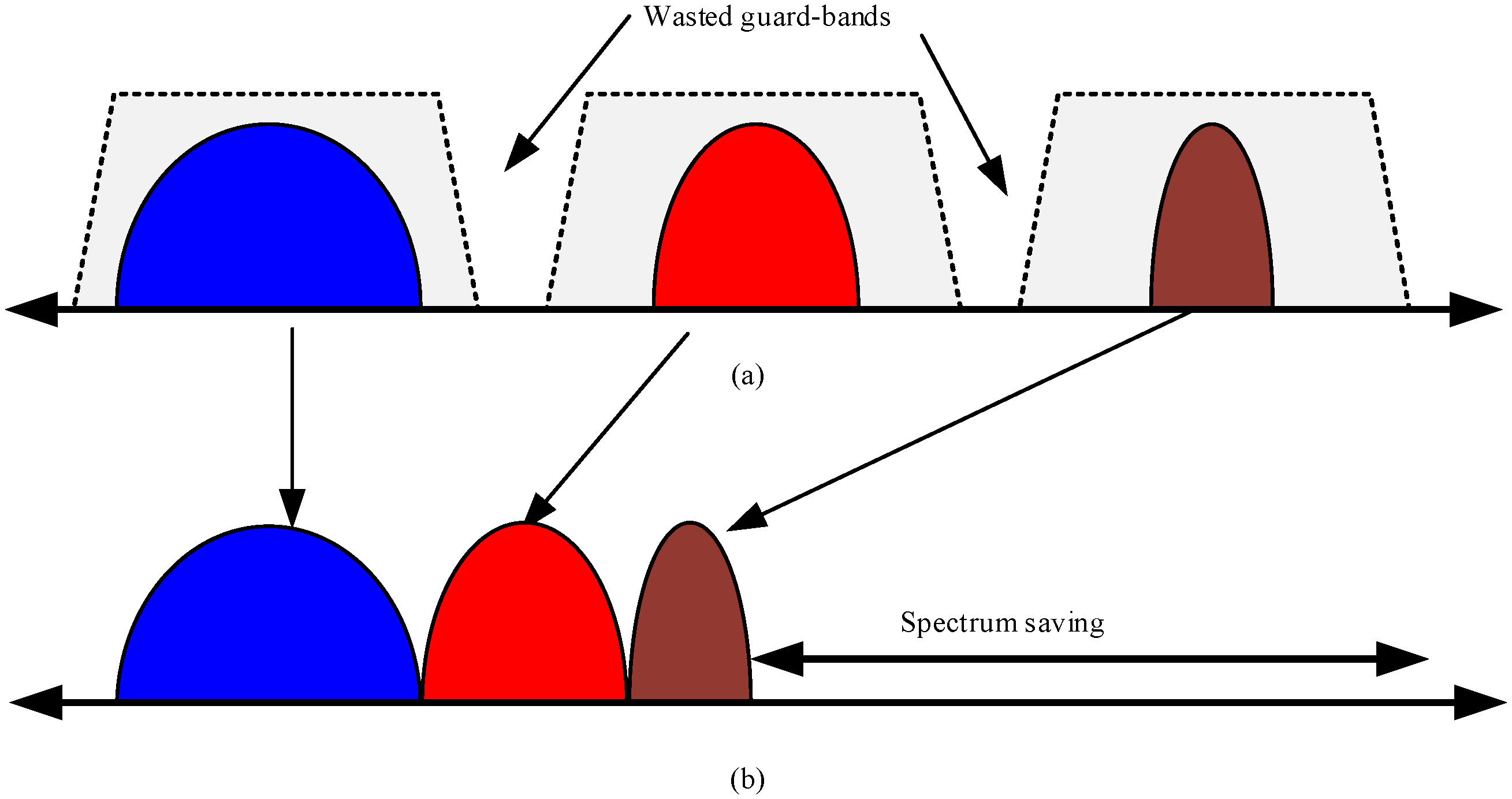
Super-channels in EONs can achieve higher spectrum efficiency compared to DWDM networks. In DWDM, the low-bandwidth services occupy less than a full wavelength causing waste in spectrum utilization as shown in Figure 2. However, super-channel networks avoid this pitfall by first eliminating the gaps between channels, and then adjusting the bandwidth using flex-grids according to fiber channel conditions.
3. Proposed OPM Techniques
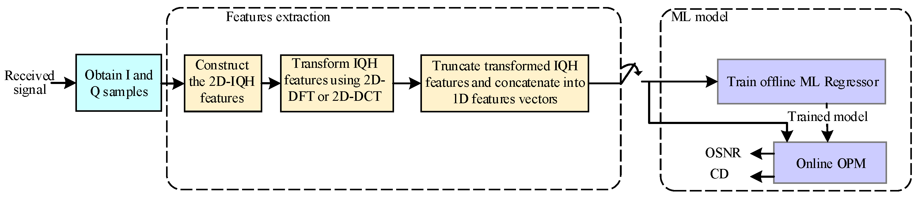
In this section, we propose a new ML-based technique for OPM in super-channel-based optical networks. Figure 3 shows the general structure of our new proposed ML-based OPM. First, the optical signal is converted to an electrical signal. Second, the resulting I and Q signals are sampled using an analog-to-digital converter (ADC). These samples are used to construct 2D-IQH features [35]. These 2D IQH features are then transformed using the 2D-DFT and 2D-DCT transforms. These transforms facilitate employing fewer samples and thus transformed 2D IQH features can be truncated and concatenated in the form of 1D features’ vectors (more details are in Section 3.1). These 1D features are then used to offline train the ML regressor (SVR in our case) to perform impairment estimation. Once the offline training is complete, the developed model and the features are then used for online OSNR and CD monitoring.
3.1. Transformed IQH Features
Previous studies [24,35] have demonstrated the effectiveness of utilizing the IQH features in OPM of single and few mode fiber (FMF) optical channels. The IQH features are built from the frequency of joint occurrence of in-phase and quadrature received samples, as demonstrated in Figure 4 for the QPSK signal at different values of OSNR, CD, and interference ratio (), defined as the ratio of the subcarrier bandwidth to subcarriers spacing. It is obvious from the figure that IQH features are sensitive to a change in the type of impairment or its level, which is a desirable property in monitoring the performance of optical channels.
Here, we propose new features extracted from applying either the 2D-DFT or 2D-DCT to the IQH samples. By doing so, fewer number of samples can be obtained to compactly represent received signal features, thereby reducing redundancy and allowing efficient utilization of ML algorithms with 1D features’ input vector. The new features are named IQH-DFT and IQH-DCT. These features along with the SVR are utilized to tackle the problem of OPM in super-channel networks. To the best of our knowledge, the problem of OPM has never been studied before for such channels. Next, the two proposed IQH-DFT and IQH-DCT features are discussed in more detail.
3.1.1. IQH-DFT Features
The 2D-DFT is widely used in image processing field; as in image filtering, image de-noising, image reconstruction, and image compression [36]. The 2D-DFT transforms an image from spatial domain into frequency domain or, in other words, it decomposes an image into components of different frequencies. Because removing some of the frequency components does not produce a noticeable effect on the quality of the original image, the 2D-DFT is often used to represent an image with a much reduced number of frequency components [37]. Since the IQH is a 2D feature, the same concept can be applied to reduce its dimensionality, and possibly to improve monitoring performance.
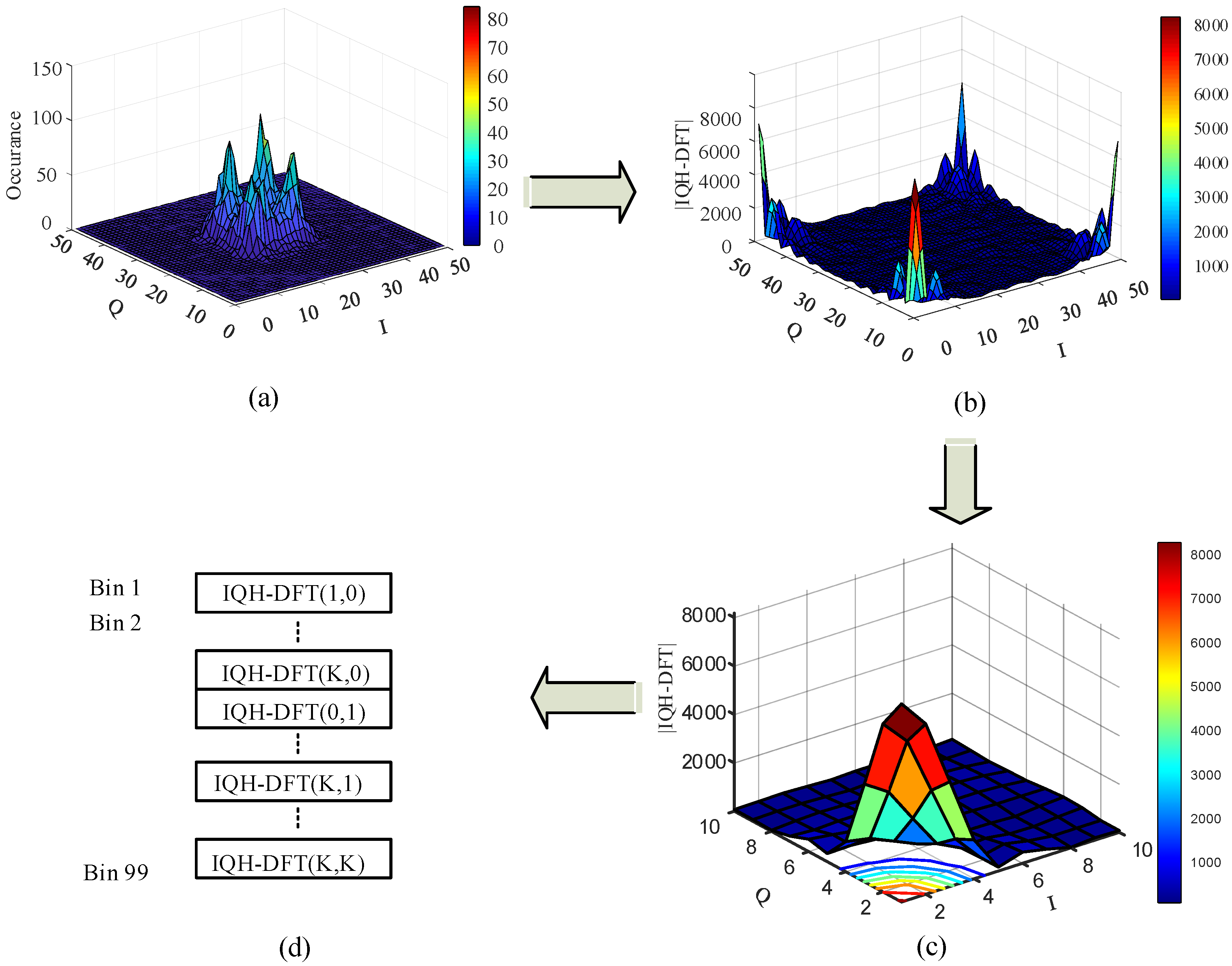
Let , where represents the IQH matrix. The IQH-DFT feature is given as
where m, n = 0,1, … K, and x, . In our development, N = 50 and K is a design parameter whose value . The proposed features’ generation method is shown in Figure 5, and can be summarized as follows:
- (a)
- (b)
- The transformed IQH features are truncated by choosing the value of K as small as possible; see, for example, Figure 5c when K = 10. In the sequel, the value of K that provides the best performance is considered. More details about the selection of value of K will be discussed in Section 5.2.
- (c)
- The truncated frequency domain features are concatenated in the form of a 1D vector after removing the DFT value at the origin (i.e., DC component). The resultant 1D features vector is denoted by V-DFT.
3.1.2. IQH-DCT Features
The 2D-DCT is the favored tool utilized in image compression, whereby it can capture more information from the image with fewer coefficients [38]. The 2D-DCT for the IQH samples can be represented mathematically as [36]
where
The 1D features vector extracted from the DCT domain (denoted by V-DCT) can be obtained in a similar manner to what has been done to generate the features vector V-DFT. The only difference is that the true values (not the magnitude) of DCT samples are considered. This is because the DCT samples are real-valued numbers (not complex). Figure 6 illustrates the generation concept of the 1D features vector, V-DCT, from the IQH of the QPSK signal.
3.2. Support Vector Regressor
SVR is one of the most popular ML regressors. For a given training dataset, X = {x1, x2, …, xM} ⊂ RD and its corresponding scalar labels y = {y1, y2, …, yM} ⊂ R1, where D is an integer ≥1 and M is the total number of samples in the training dataset. SVR attempts to find a hyperplane that best fits the dataset. SVR algorithms exploit different types of mathematical functions called kernels. Kernel functions can be either linear or nonlinear such as radial basis function (RBF), polynomial and sigmoid functions, which map the data into higher dimensional space. Comparing SVR with other kernel-based approaches, it is computationally efficient [39]. This is because it deals with a small subset of training samples called support vectors. Furthermore, it is robust to over-fitting and has the ability to reach the global minimum [40,41].
In this work, the SVR with a linear kernel is used to estimate the super-channel impairments, including OSNR and CD. The input to the SVR is the original IQH features concatenated in the form of 1D vector, V-DFT, or V-DCT. In this work, the sequential minimal optimization (SMO) algorithm has been employed to determine the optimal regressors’ parameters [42]. More details about SVR and its optimization can be found in [43,44].
4. Simulation Setup
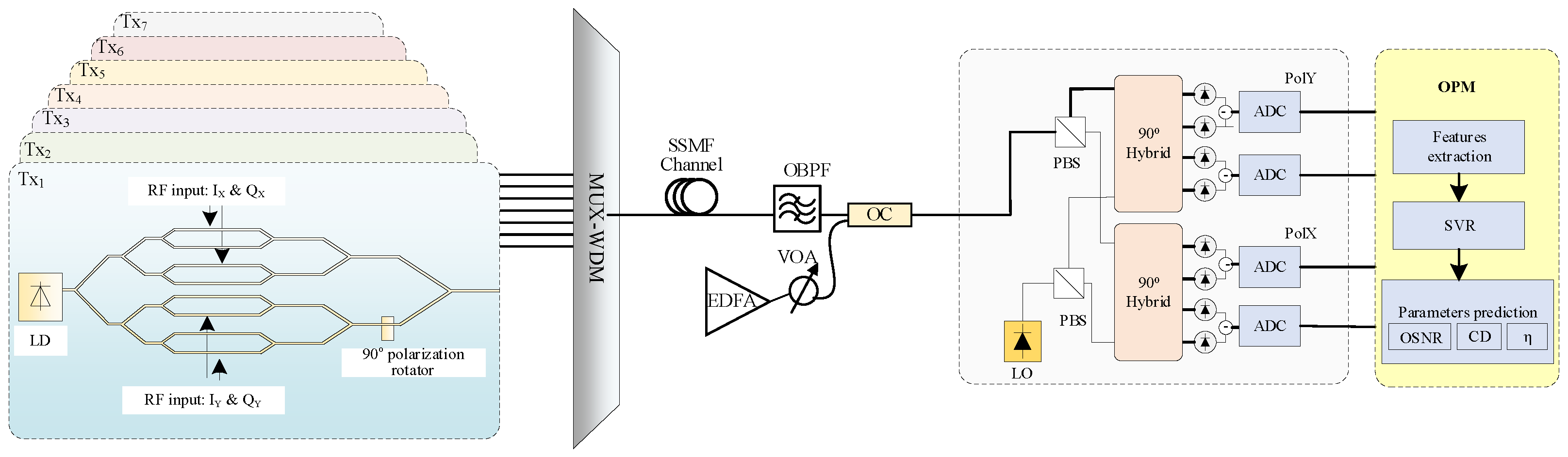
The simulation setup super-channel transceiver follows the work presented in [45] and is shown in Figure 7. A 7 × 20 Gbaud subcarriers are generated at the transmitter side. For each subcarrier, DP-QPSK at a symbol rate of 20 Gbaud is generated. The central subcarrier is operating at 1550 nm, while the wavelengths of other subcarriers are adjusted according to . The subcarriers are combined using a WDM multiplexer before transmission to an optical fiber channel. The fiber length is varied to obtain CD values in the range of 80 to 800 ps/nm. At the receiver side, one subcarrier is chosen using an optical band pass filter (OBPF). In order to add the effect of amplified spontaneous emission (ASE) noise, an erbium-doped fiber amplifier (EDFA) with a variable optical attenuator (VOA) is employed. The OSNR values are adjusted within the range of 12 to 24 dB. The received optical signal is mixed with a local oscillator (LO) to demodulate the signal. Both the received signal and LO are split into X and Y polarization components using polarization beam splitters (PBSs). Then, 90° hybrid and balanced detectors (BDs) are used to convert the mixed optical signals to electrical waveforms (IX and QX for X-Pol and (IY and QY for Y-Pol). The electrical I and Q signals are sampled using four ADCs, where the proposed OPM captures the samples directly at the output of the ADC stage. The captured samples are stored for offline processing, where 50 × 50-bin IQH features are extracted. Then, the V-DFT and V-DCT features are constructed from the transformed IQH, and used as input to the SVR.
5. Results and Discussion
In this section, we present the OPM results of the 7 × 20 Gbaud super-channel system. We generated 100 realizations for each impairment, including OSNR within the range of 12 to 24 dB (using a step of 2 dB) and CD within the range of 80 to 800 ps/nm (using a step of 80 ps/nm). The dataset is divided into 70% for training and 30% for testing, and the SVR is used to perform impairments’ estimation. Since the system subcarrier is either in the middle where it overlaps with two neighbor subcarriers, or on the side where it overlaps with only one subcarrier, we limit our study to one of each type to avoid redundancy.
The monitoring performance of three different types of features (i.e., the concatenated IQH, V-DFT, and V-DCT) is compared with the AAH features, which is taken as a reference. Note that AAH and IQH features are commonly used in literature [24,35,45,46,47,48,49,50,51,52], while V-DFT and V-DCT are our new proposed features. The effectiveness of monitoring is evaluated using visual inspection and quantitative measures. Visual inspection is performed using a standardized method called boxplot. As the boxplot width decreases, this indicates that the monitoring accuracy increases and vice versa. The coefficient of determination () is utilized as a quantitative measure, which is given as [24,53,54]
where represents the true impairment value, represents the estimate, N is the total number of impairment samples, and is the sample mean. The higher the value of is, the better the estimation. If = 1, this means a perfect match between the true and estimated values.
5.1. OPM Using Concatenated IQH Features
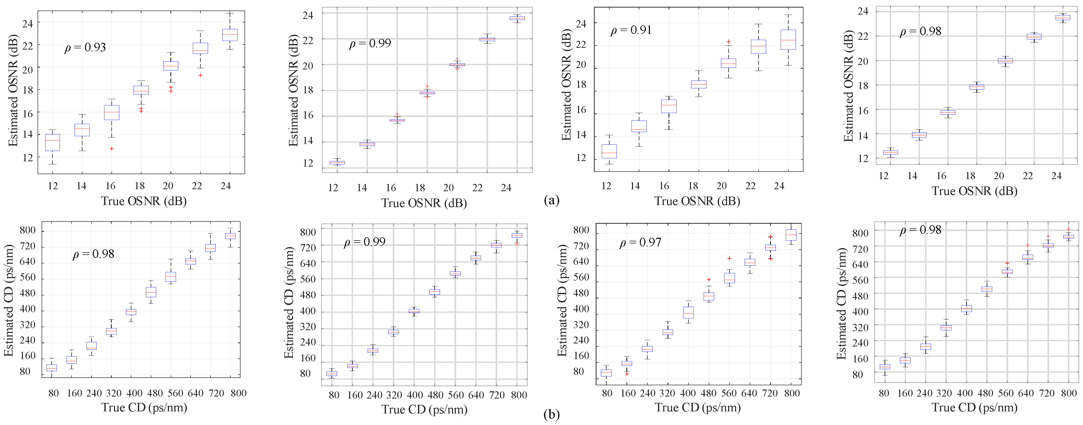
The monitoring results of OSNR and CD of the side and middle sub-carriers for both IQH and AAH features are depicted in Figure 8. The results reveal that the boxplot width of IQH, for both middle and side subcarriers, is smaller than that of AAH. Therefore, IQH features provide better estimation when compared to AAH features. These observations are further confirmed by computing the coefficient of determination for the side and middle subcarriers. For example, in the case of a side subcarrier, the coefficient of determination of AAH (IQH) for OSNR and CD are 0.93 (0.99) and 0.98 (0.99), respectively. Similarly for the middle subcarrier, the OPM accuracy of IQH features exceeds that obtained by the AAH features.
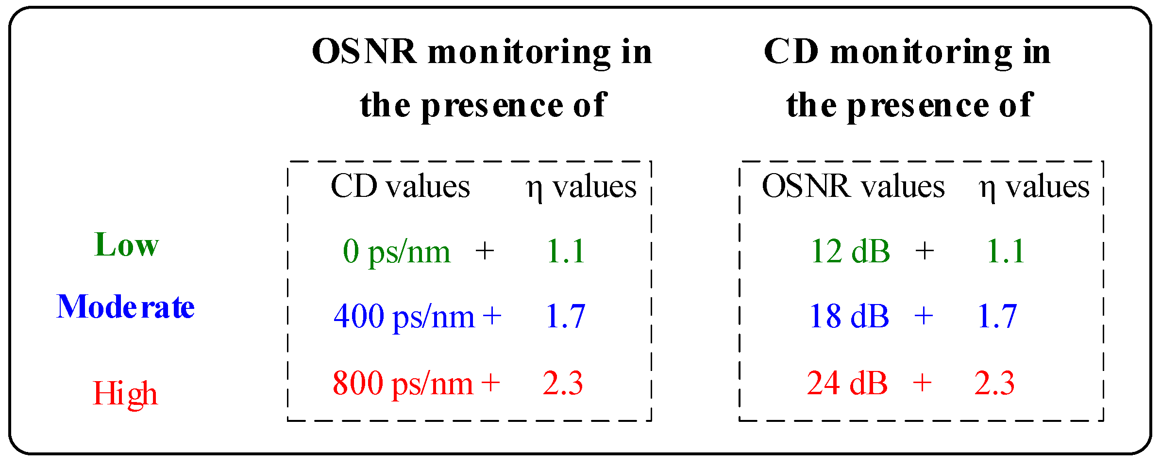
The OPM scheme using IQH with SVR is also assessed on more challenging conditions, where more than one impairment exists. Three cases for each impairment (denoted by low, moderate, and high) have been considered, as outlined in Figure 9. The OPM results are investigated in terms of (y-axis) versus the impairment type (x-axis), as shown in Figure 10.
For OSNR monitoring, the value of decreases from 0.99 and 0.98 (at = 1.1 and CD = 0 ps/nm) to 0.95 and 0.90 (at = 1.7 and CD = 400 ps/nm) for side and middle sub-carriers, respectively, as shown in Figure 10a). For high values of (i.e., = 2.3) and CD (i.e., 800 ps/nm), the monitoring accuracy in terms of decreases to 0.6 and 0.13 for side and middle sub-carriers, respectively. The reason for such a decrease in performance is owing to the high values of and CD that cause the IQH features to become cloudier, as shown in Figure 4c. Moreover, the performance of the side subcarrier is better than that of the middle subcarrier. This is because the middle subcarrier overlaps with two neighbor sub-carriers, while the side subcarrier only overlaps with one subcarrier. Similarly, for the CD, the monitoring accuracy decreases as the values of other impairments increase; see Figure 10b.
5.2. OPM Using V-DFT and V-DCT Features
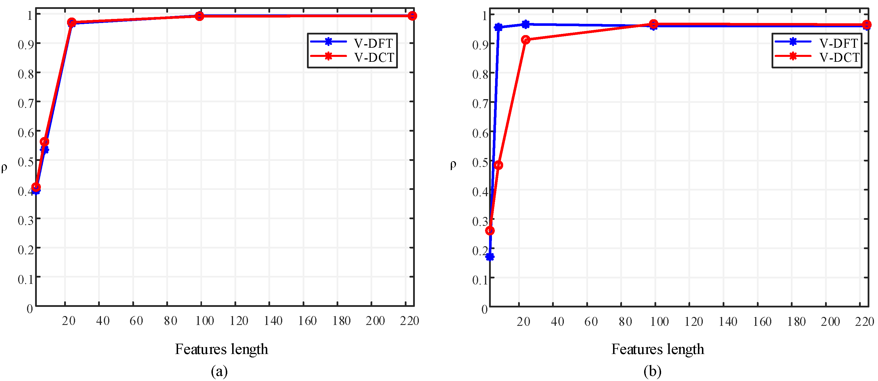
The V-DFT and V-DCT features represent the IQH in a more compact form. As discussed in Section 3.1, the optimal value of parameter K, which provides the best monitoring accuracy, needs to be selected. Towards that objective, the monitoring accuracy is evaluated at different values of K, including K = 2, 3, 5, 10, 15, which correspond to V-DFT and V-DCT features vectors of lengths 3, 5, 24, 99, 224, respectively. Figure 11 shows the monitoring results of V-DFT and V-DCT features versus the length of features vector. The results show that the monitoring accuracy almost remains unchanged as the value of K is equal to or greater than 10. Therefore, the V-DFT and V-DCT features with length ( = 99) are used in the rest of this work.
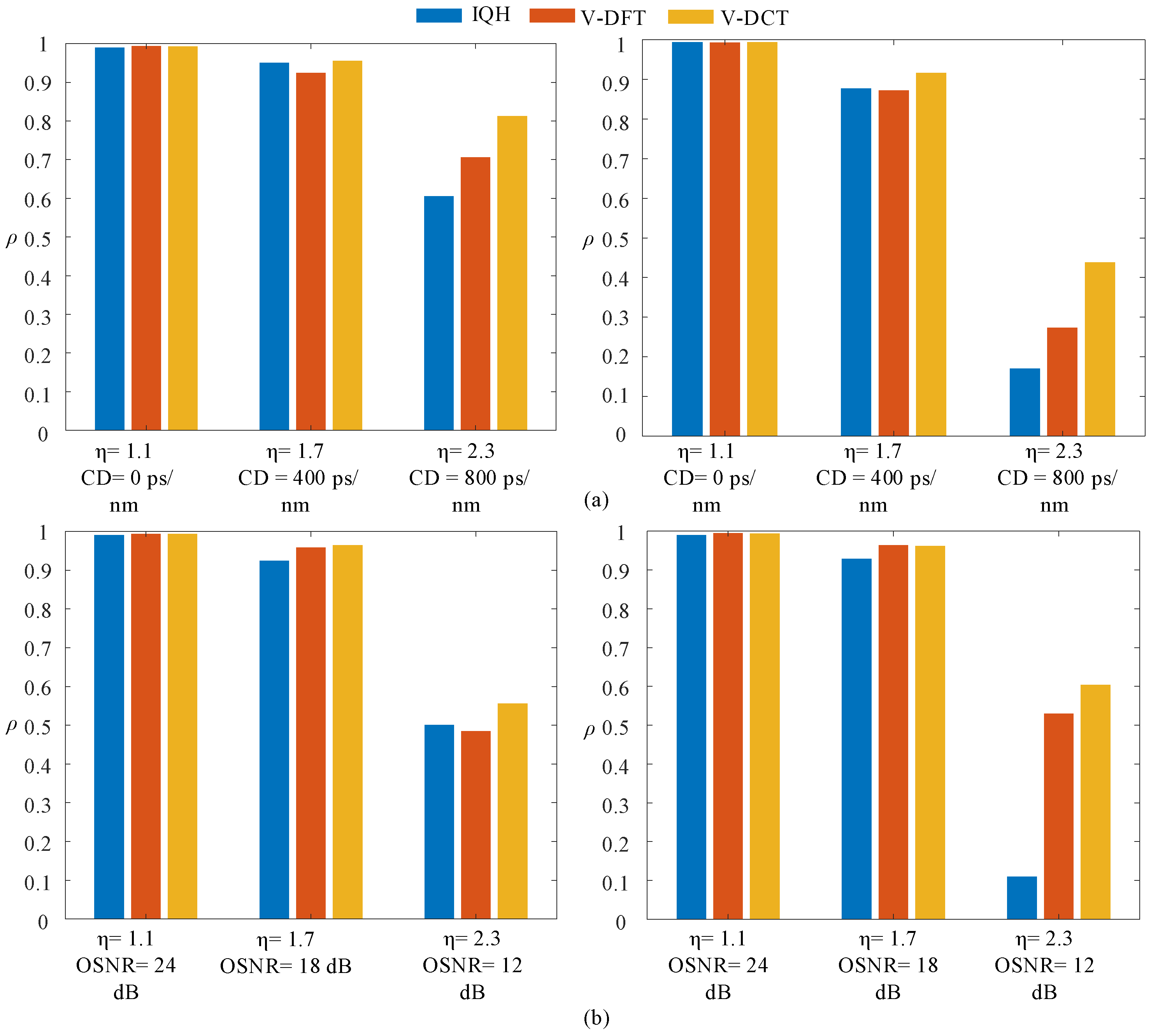
Figure 12 shows the performance of the three types of features; IQH, V-DFT, and V-DCT. It can be seen that, for OSNR and CD monitoring, and in the presence of low interference, all three features achieve the same results. As the value of increases, the V-DCT features outperform the others.
Because V-DCT features provide excellent performance compared to the other two features (i.e., IQH and V-DFT), they are used in what follows to investigate the effect of PMD, FO, and changing the type of modulation format on the OPM process in super-channel based networks. The investigation is conducted in the presence of multiple impairments, specifically, estimation of OSNR (at = 1.7 and CD = 400 ps/nm) and CD (at OSNR = 18 dB and = 1.7).
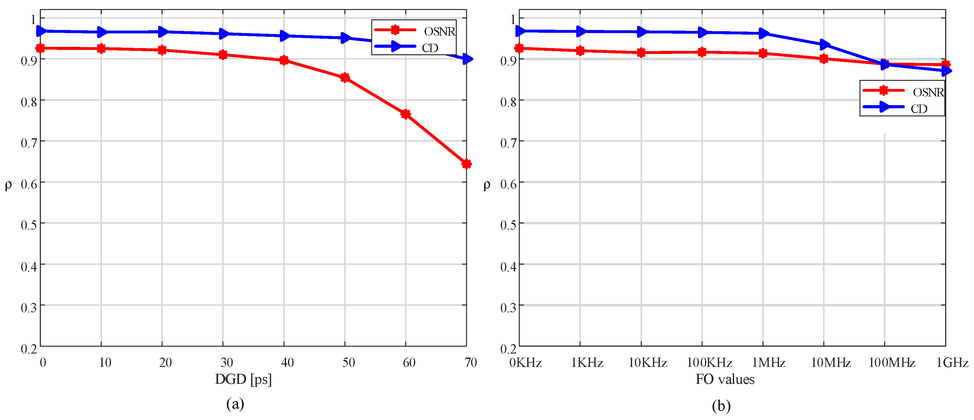
We examine the monitoring accuracy of the 1st PMD with a differential group delay (DGD) in the range of 10 to 70 ps, a state of polarization (SoP) angle of 45°, and FO ranging from 0 to 1 GHz. It is noted from Figure 13a that the OSNR accuracy has values greater than 0.9 when the DGD = 40 ps and decreases to 0.65 when the DGD reaches 70 ps. However, the CD monitoring accuracy remains greater than 0.9 even when the DGD reaches 70 ps. On the other hand, the CD monitoring accuracy almost remains unchanged even when FO reaches 1 GHz. However, the OSNR monitoring accuracy has values greater than 0.9 up to 1 MHz, and then starts decreasing and reaches 0.87 at FO = 1 GHz, as shown in Figure 13b.
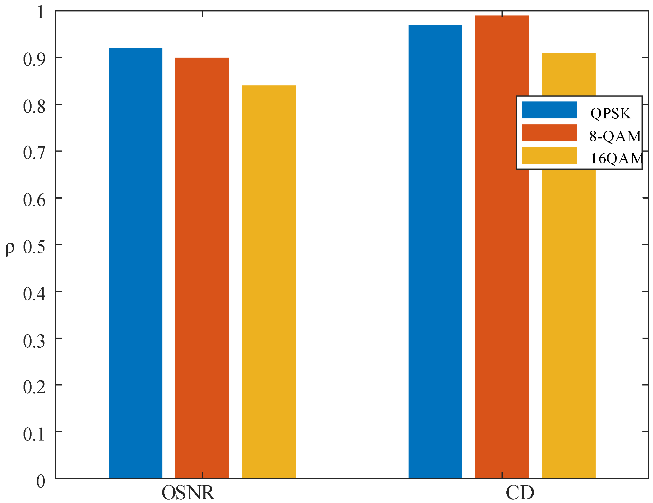
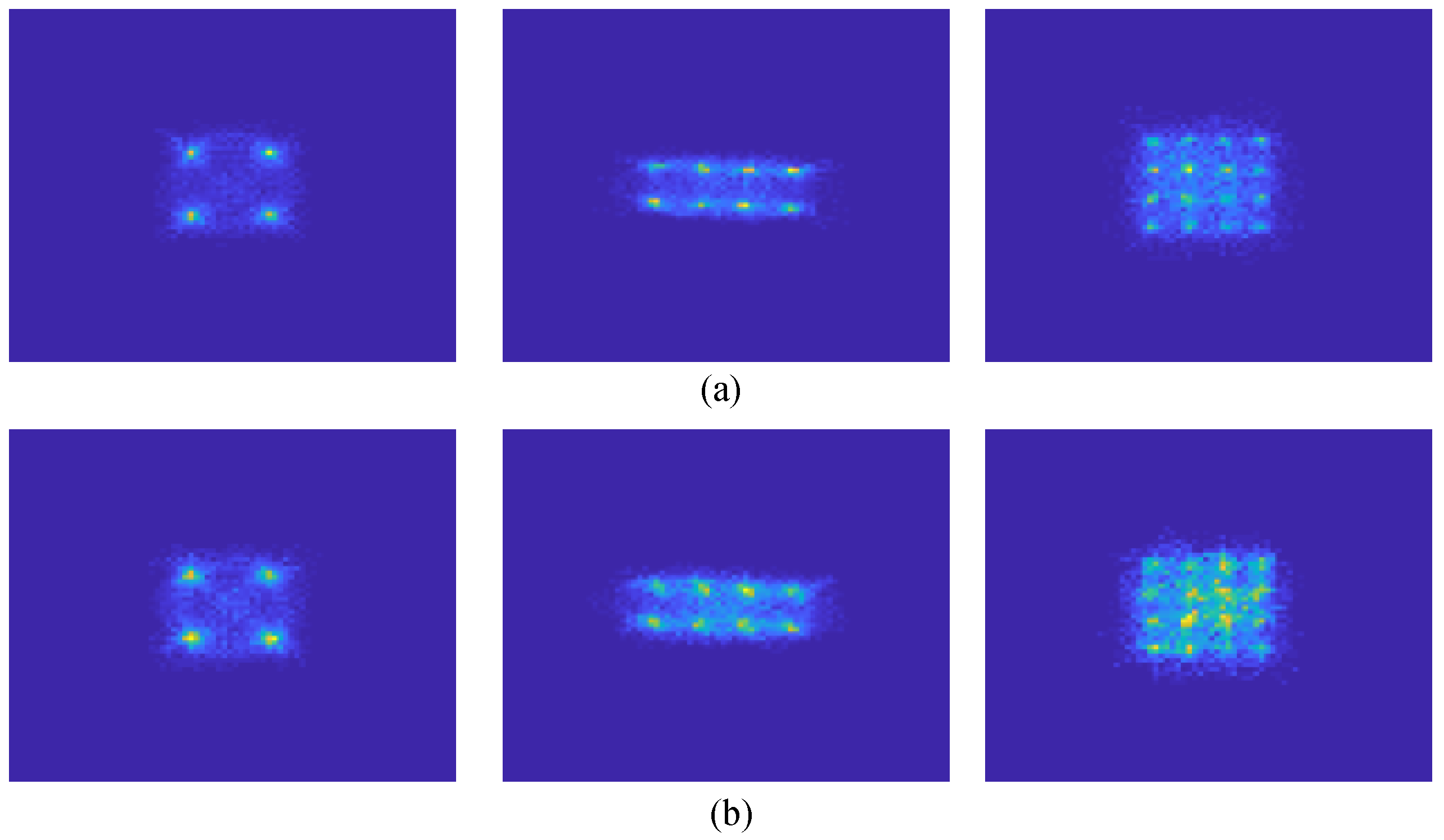
Figure 14 shows results displaying the effect of changing the modulation format on the monitoring accuracy. In this investigation, the DP-QPSK and DP-MQAM (M = 8 and 16) are considered. By virtue of Figure 14, it can be observed that, for OSNR, the accuracy decreases as modulation order increases. However, for the CD, the monitoring accuracy rises from 0.97 for DP-QPSK to 0.99 for DP-8QAM, then decreases to 0.84 for DP-16QAM. This is because the CD effect is more pronounced in DP-8QAM features than in QPSK features due to the relatively larger number of dominant IQH values, as demonstrated in Figure 15 for the case CD = 400 ps/nm. In this figure, the case of CD = 0 ps/nm is also considered for reference, and IQH features are displayed in the form of images for visualization.
On the other hand, the CD greatly affects IQH features having a larger number of dominant values as for the DP-16QAM. In this case, the features of DP-16QAM become much noisier compared to those of other two modulation formats (DP-QPSK and DP-8QAM), which in turn contributes negatively to the monitoring accuracy.
6. Experimental Validation
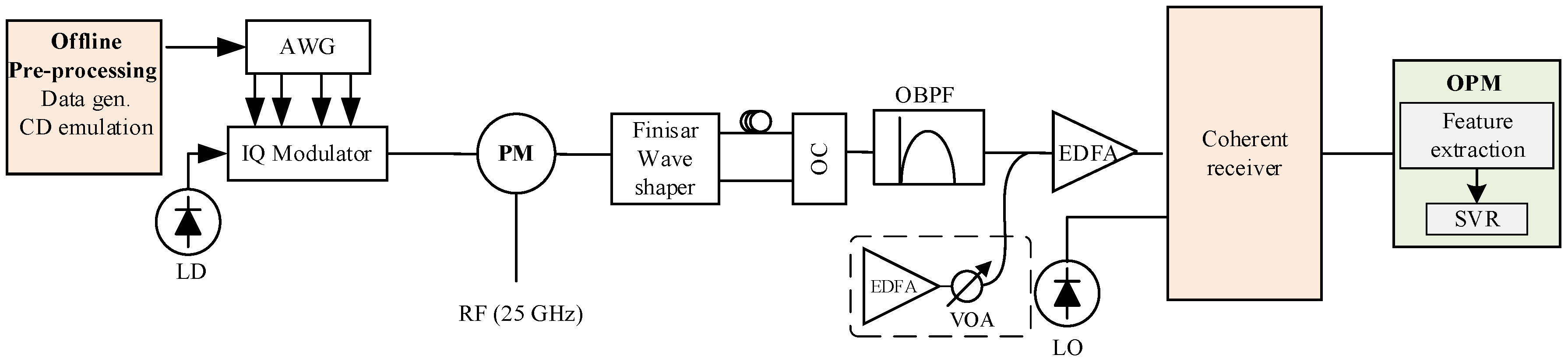
This section presents proof-of-concept experimental results to show the feasibility of the proposed OPM scheme. Figure 16 shows the setup considered to generate the signals of a super-channel transceiver, as in [45]. A narrow-linewidth distributed-feedback laser (NKT-photonics) is employed to generate optical light centered at 1550 nm. An arbitrary waveform generator (AWG) from Keysight (M8195A) with a sampling rate 64 GSa/s is used to generate electrical DP-QPSK signal. The DP-QPSK signal is modulated using the DP-IQ Mach–Zehnder modulator (DP-IQM). The modulated carrier is then applied to a frequency comb source (FCS) with 25-GHz frequency spacing, which includes RF signal source and phase modulator. A Finisar wave shaper is used to choose only seven subcarriers. These subcarriers convey the same data. Therefore, they are decorrelated by firstly separating the odd and even subcarriers, secondly delaying the even subcarriers, and finally combining the odd and delayed even subcarriers. To control the OSNR, ASE is added and adjusted using an EDFA and optical attenuator, respectively. The OSNR values are varied in the range of 12–24, with a step of 2 dB. However, the effect of CD within the range of 80 and 800 ps/nm (using a step of 80 ps/nm) is emulated electrically at the transmitter side [49,55,56]. At the receiver side, a tunable optical bandpass filter is adjusted to filter the middle subcarrier of received signal before connecting to an optical coherent receiver (N4391AKeysight optical modulation analyzer (OMA)). The acquired samples are taken directly after the analog to digital converter. These samples are used to construct the IQH, and then V-DCT features, which are used as input to the SVR.
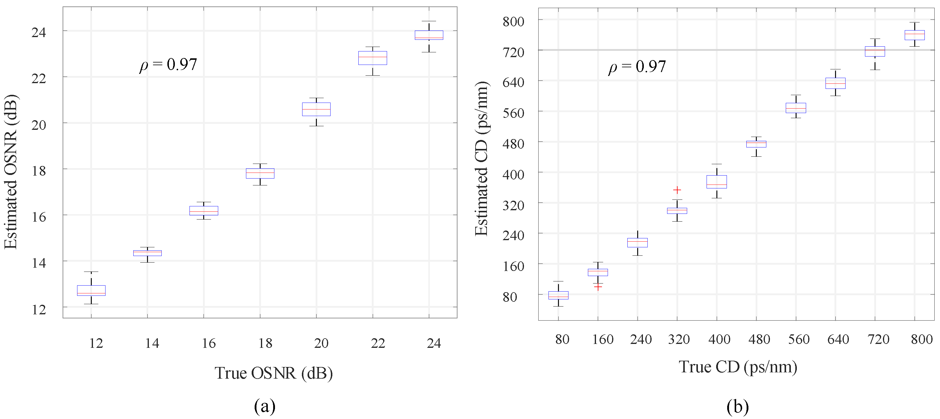
Figure 17 shows the monitoring results for OSNR (at = 1.1 and CD = 0 ps/nm) and CD (at = 1.1 and OSNR = 20). As can be observed from the figure, the coefficient of determination for both OSNR and CD is 0.97. In addition, in Figure 18, we observe excellent agreement between the simulation and experimental results.
7. Conclusions
In this paper, we demonstrated the OPM of 7 × 20 Gbaud DP-QPSK for transmission over a super-channel optical network. Two types of 1D features, including the V-DFT and V-DCT, have been proposed for the development of the OPM technique. In our development, the SVR is used to estimate the OSNR and CD. The monitoring results using the proposed V-DFT and V-DCT features are compared with those of the IQH features. The results revealed that OPM accuracy for side subcarriers outperforms that of middle subcarriers. Moreover, the results showed that the OSNR and CD can be accurately estimated for values of interference ratio up to 1.7. However, increasing the interference ratio by more than 1.7 makes the features indistinguishable for almost all different situations, which in turn destructively affects the monitoring performance. Additionally, the V-DCT based OPM scheme provides the best performance compared to the OPM techniques based on other features (i.e., AAH, IQH, and V-DFT features) and can work well even in the presence of PMD and frequency offset up 40 ps and 1 MHz, respectively. In addition, the proposed V-DCT based OPM scheme showed reasonable robustness with respect to a change in the modulation format, where its performance has been assessed using three types of modulation schemes; DP-QPSK, DP-8QAM, and DP-16QAM. Therefore, the proposed monitoring technique utilizing the V-DCT features and SVR is a promising candidate for OPM in next generation optical networks.
Author Contributions
Conceptualization, W.S.S. and S.A.A.; methodology, W.S.S. and S.A.A.; software, W.S.S. and S.A.A.; validation, W.S.S., A.M.R., B.N., T.A., M.M. and S.A.A.; investigation, W.S.S., A.M.R., B.N., T.A., M.M. and S.A.A.; writing—original draft preparation, W.S.S.; writing—review and editing, W.S.S., A.M.R., B.N., T.A., M.M. and S.A.A.; supervision, M.M. and S.A.A.; funding acquisition, S.A.A. All authors have read and agreed to the published version of the manuscript.
Funding
The authors extend their appreciation to the Deputyship for Research & Innovation, Ministry of Education in Saudi Arabia for funding this research work through the project number (DRI-KSU-1088).
Institutional Review Board Statement
Not applicable.
Informed Consent Statement
Not applicable.
Data Availability Statement
Not applicable.
Acknowledgments
The authors extend their appreciation to the Deputyship for Research & Innovation, Ministry of Education in Saudi Arabia for funding this research work.
Conflicts of Interest
The authors declare no conflict of interest.
Abbreviations
The following abbreviations are used in this manuscript:
| AAH | Asynchronous amplitude histogram |
| ADTS | Asynchronous delay-tap sampling |
| ANN | Artificial neural network |
| ASE | Amplified spontaneous emission |
| BD | Balanced detector |
| BRI | Baud rate identification |
| BVT | Bandwidth-variable transponder |
| CD | Chromatic dispersion |
| DCT | Discrete cosine transform |
| DFT | Discrete Fourier transform |
| DNN | Deep neural network |
| DP | Dual polarization |
| DWDM | Dense wavelength-division multiplexing |
| EON | Elastic optical network |
| FMF | Few mode fiber |
| FO | Frequency offset |
| IoT | Internet of things |
| IQH | In-phase quadrature histogram |
| LO | Local oscillator |
| MFI | Modulation format identification |
| ML | Machine learning |
| MTL | Multi-task learning |
| OBPF | Optical bandpass filter |
| OPM | Optical performance monitoring |
| OSNR | Optical signal-to-noise ratio |
| PBS | Polarization beam splitter |
| PMD | Polarization mode dispersion |
| RBF | Radial basis function |
| ROADM | Reconfigurable optical add-drop multiplexers |
| SMO | Sequential minimal optimization |
| SVR | Support vector regressor |
| TL | Transfer learning |
| VOA | Variable optical attenuator |
References
- Cisco. Cisco Annual Internet Report (2018–2023) White Paper; White Paper; Cisco: San Jose, CA, USA, 2020. [Google Scholar]
- Yin, Y.; Liu, L.; Proietti, R.; Yoo, S.B. Software defined elastic optical networks for cloud computing. IEEE Netw. 2016, 31, 4–10. [Google Scholar] [CrossRef]
- Winzer, P.J.; Neilson, D.T.; Chraplyvy, A.R. Fiber-optic transmission and networking: The previous 20 and the next 20 years. Opt. Express 2018, 26, 24190–24239. [Google Scholar] [CrossRef] [PubMed]
- Gerstel, O.; Jinno, M.; Lord, A.; Yoo, S.B. Elastic optical networking: A new dawn for the optical layer? IEEE Commun. Mag. 2012, 50, s12–s20. [Google Scholar] [CrossRef]
- Chatterjee, B.C.; Oki, E. Elastic Optical Networks: Fundamentals, Design, Control, and Management: Fundamentals, Design, Control, and Management; CRC Press: Boca Raton, FL, USA, 2020. [Google Scholar]
- Dong, Z.; Khan, F.N.; Sui, Q.; Zhong, K.; Lu, C.; Lau, A.P.T. Optical performance monitoring: A review of current and future technologies. J. Light. Technol. 2015, 34, 525–543. [Google Scholar] [CrossRef]
- Willner, A.E.; Pan, Z.; Yu, C. Optical performance monitoring. In Optical Fiber Telecommunications VB; Elsevier: Amsterdam, The Netherlands, 2008; pp. 233–292. [Google Scholar]
- Wang, D.; Sui, Q.; Li, Z. Toward universal optical performance monitoring for intelligent optical fiber communication networks. IEEE Commun. Mag. 2020, 58, 54–59. [Google Scholar] [CrossRef]
- Wang, D.; Jiang, H.; Liang, G.; Zhan, Q.; Mo, Y.; Sui, Q.; Li, Z. Optical Performance Monitoring of Multiple Parameters in Future Optical Networks. J. Light. Technol. 2021, 39, 3792–3800. [Google Scholar] [CrossRef]
- Suzuki, H.; Takachio, N. Optical signal quality monitor built into WDM linear repeaters using semiconductor arrayed waveguide grating filter monolithically integrated with eight photodiodes. Electron. Lett. 1999, 35, 836–837. [Google Scholar] [CrossRef]
- Lee, J.; Choi, H.; Shin, S.; Chung, Y.C. A review of the polarization-nulling technique for monitoring optical-signal-to-noise ratio in dynamic WDM networks. J. Light. Technol. 2006, 24, 4162–4171. [Google Scholar] [CrossRef]
- Liu, X.; Kao, Y.H.; Chandrasekhar, S.; Kang, I.; Cabot, S.; Buhl, L. OSNR monitoring method for OOK and DPSK based on optical delay interferometer. IEEE Photonics Technol. Lett. 2007, 19, 1172–1174. [Google Scholar] [CrossRef]
- Flood, E.; Guo, W.; Reid, D.; Lynch, M.; Bradley, A.; Barry, L.; Donegan, J. In-band OSNR monitoring using a pair of Michelson fiber interferometers. Opt. Express 2010, 18, 3618–3625. [Google Scholar] [CrossRef]
- Ji, T.; Peng, Y.; Zhu, G. In-band OSNR monitoring from Stokes parameters using support vector regression. IEEE Photonics Technol. Lett. 2019, 31, 385–388. [Google Scholar] [CrossRef]
- Xu, K.; Tsang, H.K.; Lei, G.K.; Chen, Y.M.; Wang, L.; Cheng, Z.; Chen, X.; Shu, C. OSNR monitoring for NRZ-PSK signals using silicon waveguide two-photon absorption. IEEE Photonics J. 2011, 3, 968–974. [Google Scholar] [CrossRef]
- Yu, Q.; Pan, Z.; Yan, L.S.; Willner, A.E. Chromatic dispersion monitoring technique using sideband optical filtering and clock phase-shift detection. J. Light. Technol. 2002, 20, 2267–2271. [Google Scholar]
- Zaidi, A.; Estella-Aguerri, I.; Shamai, S. On the information bottleneck problems: Models, connections, applications and information theoretic views. Entropy 2020, 22, 151. [Google Scholar] [CrossRef] [PubMed] [Green Version]
- Farsad, N.; Yilmaz, H.B.; Eckford, A.; Chae, C.B.; Guo, W. A Comprehensive survey of recent advancements in molecular communication. IEEE Commun. Surv. Tutor. 2016, 18, 1887–1919. [Google Scholar] [CrossRef] [Green Version]
- Wang, X.; Gao, L.; Mao, S.; Pandey, S. CSI-Based fingerprinting for indoor localization: A deep learning approach. IEEE Trans. Veh. Technol. 2017, 66, 763–776. [Google Scholar] [CrossRef] [Green Version]
- Aguerri, I.E.; Zaidi, A. Distributed variational representation learning. IEEE Trans. Pattern Anal. Mach. Intell. 2021, 43, 120–138. [Google Scholar] [CrossRef] [Green Version]
- Saif, W.S.; Esmail, M.A.; Ragheb, A.M.; Alshawi, T.A.; Alshebeili, S.A. Machine Learning Techniques for Optical Performance Monitoring and Modulation Format Identification: A Survey. IEEE Commun. Surv. Tutor. 2020, 22, 2839–2882. [Google Scholar] [CrossRef]
- Khan, F.N.; Fan, Q.; Lu, C.; Lau, A.P.T. An optical communication’s perspective on machine learning and its applications. J. Light. Technol. 2019, 37, 493–516. [Google Scholar] [CrossRef]
- Musumeci, F.; Rottondi, C.; Nag, A.; Macaluso, I.; Zibar, D.; Ruffini, M.; Tornatore, M. An overview on application of machine learning techniques in optical networks. IEEE Commun. Surv. Tutor. 2018, 21, 1383–1408. [Google Scholar] [CrossRef] [Green Version]
- Saif, W.S.; Ragheb, A.M.; Alshawi, T.A.; Alshebeili, S.A. Optical Performance Monitoring in Mode Division Multiplexed Optical Networks. J. Light. Technol. 2020, 39, 491–504. [Google Scholar] [CrossRef]
- Khan, F.N.; Lu, C.; Lau, A.P.T. Optical performance monitoring in fiber-optic networks enabled by machine learning techniques. In Proceedings of the Optical Fiber Communications Conference and Exposition (OFC), San Diego, CA, USA, 7–9 March 2018; pp. 1–3. [Google Scholar]
- Xiang, Q.; Yang, Y.; Zhang, Q.; Yao, Y. Joint and accurate OSNR estimation and modulation format identification scheme using the feature-based ANN. IEEE Photonics J. 2019, 11, 1–11. [Google Scholar] [CrossRef]
- Mata, J.; de Miguel, I.; Duran, R.J.; Merayo, N.; Singh, S.K.; Jukan, A.; Chamania, M. Artificial intelligence (AI) methods in optical networks: A comprehensive survey. Opt. Switch. Netw. 2018, 28, 43–57. [Google Scholar] [CrossRef]
- Wu, X.; Jargon, J.A.; Skoog, R.A.; Paraschis, L.; Willner, A.E. Applications of artificial neural networks in optical performance monitoring. J. Light. Technol. 2009, 27, 3580–3589. [Google Scholar]
- Shen, T.S.R.; Meng, K.; Lau, A.P.T.; Dong, Z.Y. Optical performance monitoring using artificial neural network trained with asynchronous amplitude histograms. IEEE Photonics Technol. Lett. 2010, 22, 1665–1667. [Google Scholar] [CrossRef]
- Jargon, J.A.; Wu, X.; Willner, A.E. Optical performance monitoring by use of artificial neural networks trained with parameters derived from delay-tap asynchronous sampling. In Proceedings of the 2009 Conference on Optical Fiber Communication, San Diego, CA, USA, 22–26 March 2009; pp. 1–3. [Google Scholar]
- Cheng, Y.; Fu, S.; Tang, M.; Liu, D. Multi-task deep neural network (MT-DNN) enabled optical performance monitoring from directly detected PDM-QAM signals. Opt. Express 2019, 27, 19062–19074. [Google Scholar] [CrossRef] [PubMed]
- Luo, H.; Huang, Z.; Wu, X.; Yu, C. Cost-Effective Multi-Parameter Optical Performance Monitoring Using Multi-Task Deep Learning With Adaptive ADTP and AAH. J. Light. Technol. 2021, 39, 1733–1741. [Google Scholar] [CrossRef]
- Xia, L.; Zhang, J.; Hu, S.; Zhu, M.; Song, Y.; Qiu, K. Transfer learning assisted deep neural network for OSNR estimation. Opt. Express 2019, 27, 19398–19406. [Google Scholar] [CrossRef]
- Tanimura, T.; Hoshida, T.; Kato, T.; Watanabe, S.; Rasmussen, J.C.; Suzuki, M.; Morikawa, H. Deep learning based OSNR monitoring independent of modulation format, symbol rate and chromatic dispersion. In Proceedings of the 42nd European Conference on Optical Communication (ECOC 2016), Dusseldorf, Germany, 18–22 September 2016; pp. 1–3. [Google Scholar]
- Saif, W.S.; Alshawi, T.; Esmail, M.A.; Ragheb, A.; Alshebeili, S. Separability of histogram based features for optical performance monitoring: An investigation using t-SNE technique. IEEE Photonics J. 2019, 11, 1–12. [Google Scholar] [CrossRef]
- Gonzalez, R.; Woods, R. Digital Image Processing; Pearson: New York, NY, USA, 2018. [Google Scholar]
- Rasheed, M.H.; Salih, O.M.; Siddeq, M.M.; Rodrigues, M.A. Image compression based on 2D Discrete Fourier Transform and matrix minimization algorithm. Array 2020, 6, 100024. [Google Scholar] [CrossRef]
- Jain, A.K. Fundamentals of Digital Image Processing; Prentice-Hall, Inc.: Englewood Cliffs, NJ, USA, 1989. [Google Scholar]
- Thrane, J.; Wass, J.; Piels, M.; Diniz, J.C.M.; Jones, R.; Zibar, D. Machine Learning Techniques for Optical Performance Monitoring From Directly Detected PDM-QAM Signals. J. Light. Technol. 2017, 35, 868–875. [Google Scholar] [CrossRef] [Green Version]
- Lin, X.; Dobre, O.A.; Ngatched, T.M.N.; Eldemerdash, Y.A.; Li, C. Joint Modulation Classification and OSNR Estimation Enabled by Support Vector Machine. IEEE Photonics Technol. Lett. 2018, 30, 2127–2130. [Google Scholar] [CrossRef]
- Vapnik, V.N. An overview of statistical learning theory. IEEE Transactions on Neural Networks 1999, 10, 988–999. [Google Scholar] [CrossRef] [PubMed] [Green Version]
- Platt, J. Sequential Minimal Optimization: A Fast Algorithm for Training Support Vector Machines; Technical Report MSR-TR-98-14, Advances in Kernel Methods—Support Vector Learning; Microsoft: Redmond, WA, USA, 1998. [Google Scholar]
- Vapnik, V. The Nature of Statistical Learning Theory; Springer: New York, NY, USA, 2000. [Google Scholar]
- Hearst, M.; Dumais, S.; Osuna, E.; Platt, J.; Scholkopf, B. Support vector machines: A practical consequence of learning theory. IEEE Intell. Syst. 1998, 13, 18–28. [Google Scholar] [CrossRef] [Green Version]
- Saif, W.S.; Ragheb, A.M.; Nebendahl, B.; Alshawi, T.; Marey, M.; Alshebeili, S.A. Performance Investigation of Modulation Format Identification in Super-Channel Optical Networks. IEEE Photonics J. 2022, 14, 1–10. [Google Scholar] [CrossRef]
- Khan, F.N.; Zhou, Y.; Lau, A.P.T.; Lu, C. Modulation format identification in heterogeneous fiber-optic networks using artificial neural networks. Opt. Express 2012, 20, 12422–12431. [Google Scholar] [CrossRef] [Green Version]
- Khan, F.N.; Zhong, K.; Al-Arashi, W.H.; Yu, C.; Lu, C.; Lau, A.P.T. Modulation format identification in coherent receivers using deep machine learning. IEEE Photonics Technol. Lett. 2016, 28, 1886–1889. [Google Scholar] [CrossRef]
- Khan, F.N.; Zhong, K.; Zhou, X.; Al-Arashi, W.H.; Yu, C.; Lu, C.; Lau, A.P.T. Joint OSNR monitoring and modulation format identification in digital coherent receivers using deep neural networks. Opt. Express 2017, 25, 17767–17776. [Google Scholar] [CrossRef]
- Guesmi, L.; Ragheb, A.M.; Fathallah, H.; Menif, M. Experimental Demonstration of Simultaneous Modulation Format/Symbol Rate Identification and Optical Performance Monitoring for Coherent Optical Systems. J. Light. Technol. 2018, 36, 2230–2239. [Google Scholar] [CrossRef]
- Zhao, Y.; Shi, C.; Wang, D.; Chen, X.; Wang, L.; Yang, T.; Du, J. Low-complexity and nonlinearity-tolerant modulation format identification using random forest. IEEE Photonics Technol. Lett. 2019, 31, 853–856. [Google Scholar] [CrossRef]
- Wan, Z.; Yu, Z.; Shu, L.; Zhao, Y.; Zhang, H.; Xu, K. Intelligent optical performance monitor using multi-task learning based artificial neural network. Opt. Express 2019, 27, 11281–11291. [Google Scholar] [CrossRef] [Green Version]
- Saif, W.S.; Ragheb, A.M.; Seleem, H.E.; Alshawi, T.A.; Alshebeili, S.A. Modulation format identification in mode division multiplexed optical networks. IEEE Access 2019, 7, 156207–156216. [Google Scholar] [CrossRef]
- Kva, T.O. Note on the R2 measure of goodness of fit for nonlinear models. Bull. Psychon. Soc. 1983, 21, 79–80. [Google Scholar]
- Esmail, M.A.; Saif, W.S.; Ragheb, A.M.; Alshebeili, S.A. Free space optic channel monitoring using machine learning. Opt. Express 2021, 29, 10967–10981. [Google Scholar] [CrossRef]
- Tanimura, T.; Hoshida, T.; Kato, T.; Watanabe, S.; Morikawa, H. Convolutional neural network-based optical performance monitoring for optical transport networks. J. Opt. Commun. Netw. 2019, 11, A52–A59. [Google Scholar] [CrossRef]
- Eltaieb, R.A.; Farghal, A.E.A.; Ahmed, H.d.H.; Saif, W.S.; Ragheb, A.; Alshebeili, S.A.; Shalaby, H.M.H.; Abd El-Samie, F.E. Efficient Classification of Optical Modulation Formats Based on Singular Value Decomposition and Radon Transformation. J. Light. Technol. 2020, 38, 619–631. [Google Scholar] [CrossRef]
Figure 1.
Basic principle of OPM in next generation EONs. Here, BVT is the bandwidth-variable transponder and ROADM is reconfigurable optical add/drop multiplexers.
Figure 1.
Basic principle of OPM in next generation EONs. Here, BVT is the bandwidth-variable transponder and ROADM is reconfigurable optical add/drop multiplexers.

Figure 2.
Optical spectrum for (a) DWDM and (b) super-channel networks.

Figure 3.
Schematic diagram for our proposed OPM using ML techniques.

Figure 4.
IQH-based features for QPSK signal at different OSNR values (i.e., left (12 dB), middle (18 dB), and (24 dB)) at: (a) CD = 80 ps/nm and interference ratio = 1.1; (b) CD = 400 ps/nm and interference ratio = 1.7; and (c) CD = 800 ps/nm and interference ratio = 2.3.
Figure 4.
IQH-based features for QPSK signal at different OSNR values (i.e., left (12 dB), middle (18 dB), and (24 dB)) at: (a) CD = 80 ps/nm and interference ratio = 1.1; (b) CD = 400 ps/nm and interference ratio = 1.7; and (c) CD = 800 ps/nm and interference ratio = 2.3.

Figure 5.
The concept of generating the 1D features vector, V-DFT, from the IQH of the QPSK signal. (a) IQH features, (b) IQH-DFT features, (c) Truncated IQH-DFT, (d) V-DFT features.
Figure 5.
The concept of generating the 1D features vector, V-DFT, from the IQH of the QPSK signal. (a) IQH features, (b) IQH-DFT features, (c) Truncated IQH-DFT, (d) V-DFT features.

Figure 6.
The concept of generating the 1D features vector, V-DCT, from the IQH of the QPSK signal. (a) IQH features, (b) IQH-DCT features, (c) Truncated IQH-DCT, (d) V-DCT features.
Figure 6.
The concept of generating the 1D features vector, V-DCT, from the IQH of the QPSK signal. (a) IQH features, (b) IQH-DCT features, (c) Truncated IQH-DCT, (d) V-DCT features.

Figure 7.
Simulation setup of the proposed OPM in super-channel networks. LD: laser diode, EDFA: Erbium-doped fiber amplifier, VOA: variable optical attenuator, WDM: wavelength division multiplexing, MUX: multiplexer, OBPF: optical band pass filter, PBS: polarization beam splitter, OC: optical coupler, ADC: analog to digital convertor, LO: local oscillator, SVR: support vector regressor, : interference ratio, OPM: optical performance monitoring.

Figure 8.
OPM results using AAH (1st column and 3rd column ) and IQH (2nd column and 4th column) with SVR for side (1st column and 2nd column) and middle (3rd column and 4th column) sub-carriers (a) OSNR and (b) CD.
Figure 8.
OPM results using AAH (1st column and 3rd column ) and IQH (2nd column and 4th column) with SVR for side (1st column and 2nd column) and middle (3rd column and 4th column) sub-carriers (a) OSNR and (b) CD.

Figure 9.
Monitoring scenarios for different impairments.

Figure 10.
OPM results using IQH with SVR of side and middle sub-carriers (a) OSNR monitoring and (b) CD monitoring.
Figure 10.
OPM results using IQH with SVR of side and middle sub-carriers (a) OSNR monitoring and (b) CD monitoring.

Figure 11.
Examples of monitoring results as a function of IQH-DFT and IQH-DCT features lengths: (a) OSNR monitoring at = 1.1 and CD = 0 ps/nm; (b) CD monitoring at = 1.1 and OSNR = 24 dB.
Figure 11.
Examples of monitoring results as a function of IQH-DFT and IQH-DCT features lengths: (a) OSNR monitoring at = 1.1 and CD = 0 ps/nm; (b) CD monitoring at = 1.1 and OSNR = 24 dB.

Figure 12.
Comparisons between monitoring results using different feature types of both side (left) and middle (right) sub-carriers: (a) OSNR monitoring and (b) CD monitoring.
Figure 12.
Comparisons between monitoring results using different feature types of both side (left) and middle (right) sub-carriers: (a) OSNR monitoring and (b) CD monitoring.

Figure 13.
OPM results using V-DCT at different values of (a) FO and (b) PMD.

Figure 14.
OPM results using V-DCT features and different modulation formats.

Figure 15.
Images of IQH features of QPSK (1st column), 8QAM (2nd column), and 16QAM (3rd column) at: (a) CD= 0 ps/nm; (b) CD = 400 ps/nm.
Figure 15.
Images of IQH features of QPSK (1st column), 8QAM (2nd column), and 16QAM (3rd column) at: (a) CD= 0 ps/nm; (b) CD = 400 ps/nm.

Figure 16.
Experimental setup of the proposed OPM in super-channel networks. LD: laser diode, AWG: arbitrary waveform generator, RF: radio frequency, PM: phase modulator, EDFA: Erbium-doped fiber amplifier, VOA: variable optical attenuator, OSNR: optical signal-to-noise ratio, OBPF: optical band pass filter, OC: optical coupler, LO: local oscillator.

Figure 17.
OPM experimental results for (a) OSNR and (b) CD.

Figure 18.
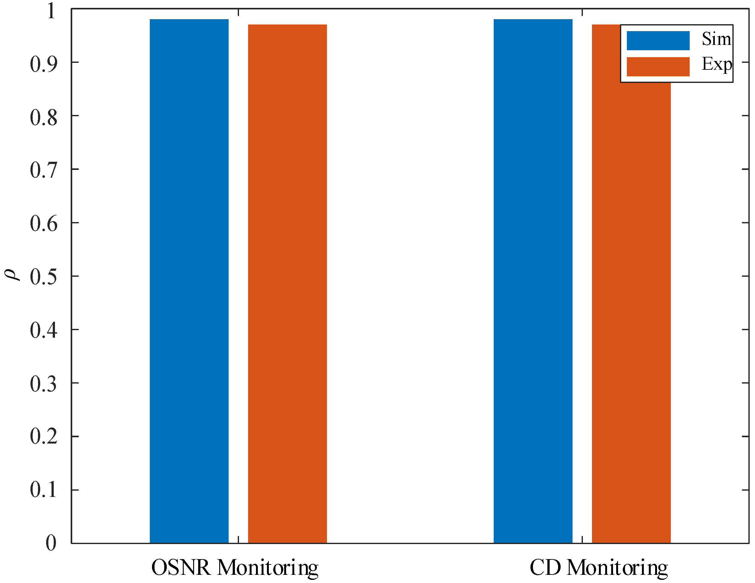
Simulation vs. experimental results for monitoring OSNR and CD.

Publisher’s Note: MDPI stays neutral with regard to jurisdictional claims in published maps and institutional affiliations. |
© 2022 by the authors. Licensee MDPI, Basel, Switzerland. This article is an open access article distributed under the terms and conditions of the Creative Commons Attribution (CC BY) license (https://creativecommons.org/licenses/by/4.0/).
Share and Cite
MDPI and ACS Style
Saif, W.S.; Ragheb, A.M.; Nebendahl, B.; Alshawi, T.; Marey, M.; Alshebeili, S.A. Machine Learning-Based Optical Performance Monitoring for Super-Channel Optical Networks. Photonics 2022, 9, 299. https://doi.org/10.3390/photonics9050299
AMA Style
Saif WS, Ragheb AM, Nebendahl B, Alshawi T, Marey M, Alshebeili SA. Machine Learning-Based Optical Performance Monitoring for Super-Channel Optical Networks. Photonics. 2022; 9(5):299. https://doi.org/10.3390/photonics9050299
Chicago/Turabian StyleSaif, Waddah S., Amr M. Ragheb, Bernd Nebendahl, Tariq Alshawi, Mohamed Marey, and Saleh A. Alshebeili. 2022. "Machine Learning-Based Optical Performance Monitoring for Super-Channel Optical Networks" Photonics 9, no. 5: 299. https://doi.org/10.3390/photonics9050299
Note that from the first issue of 2016, this journal uses article numbers instead of page numbers. See further details here.