All articles published by MDPI are made immediately available worldwide under an open access license. No special
permission is required to reuse all or part of the article published by MDPI, including figures and tables. For
articles published under an open access Creative Common CC BY license, any part of the article may be reused without
permission provided that the original article is clearly cited. For more information, please refer to
https://www.mdpi.com/openaccess.
Feature papers represent the most advanced research with significant potential for high impact in the field. A Feature
Paper should be a substantial original Article that involves several techniques or approaches, provides an outlook for
future research directions and describes possible research applications.
Feature papers are submitted upon individual invitation or recommendation by the scientific editors and must receive
positive feedback from the reviewers.
Editor’s Choice articles are based on recommendations by the scientific editors of MDPI journals from around the world.
Editors select a small number of articles recently published in the journal that they believe will be particularly
interesting to readers, or important in the respective research area. The aim is to provide a snapshot of some of the
most exciting work published in the various research areas of the journal.
The intermediate-band solar cell (IBSC) has been proposed as a high-efficiency solar cell because of the extended absorption it allows for, which results from the intermediate band. In order to further increase the efficiency of IBSCs, we study a novel device with dual intermediate bands. Because of the extended absorption from the second intermediate band, the efficiency of a dual IBSC can reach 86.5% at a full concentration. Moreover, we study the performance of the IBSC based on InAs/InGaAs quantum dots. The efficiency of the device is shown to be able to reach 74.4% when the In composition is 75%. In addition, the transition process between the dual intermediate bands greatly affects the efficiency, so it is important to design the dual intermediate bands in a precise manner.
In order to improve the efficiency of solar cells and overcome the Schockley–Queisser limit, researchers have proposed many new theories and technologies. These include the intermediate-band solar cell (IBSC), with a detailed balance-limiting efficiency of 63.2% compared to 40.7% for a single-junction solar cell at full concentration; when compared with tandem cells, the IBSC can not only achieve multispectral absorption, but can also achieve higher efficiency because it is not limited by current matching conditions [1,2,3,4]. Even under one sun, the IBSC can achieve an efficiency of 46.8% instead of 31% for a single-junction solar cell [1,4]. The IBSC achieves ultra-high efficiency because it introduces an additional energy band that lies within the normal bandgap. Therefore, it breaks through the limitation of the traditional bandgap and creates extra photon absorption through the sequential absorption of the two sub-bandgaps, which greatly broadens the absorption of the solar spectrum. The IBSC is regarded as the third generation of solar cells that breaks the limiting efficiency of traditional photovoltaic devices [5,6]. The IBSC, with an efficiency of 63.2%, is inserted at an intermediate level of 0.71 eV below the conduction band into a material with a bandgap of 1.95 eV [7], which means that it is unable to absorb photons below 0.71 eV. However, the number of such photons is considerable, which ultimately makes the IBSC fail to surpass the limiting efficiency of 63.2%. Some researchers also proposed the concept of a photon ratchet IBSC; however, in terms of the photon absorption process, it is still essentially a solar cell with a single intermediate band, and the ratchet band focuses on increasing the lifetime of carriers [4,8].
Although the IBSC is attractive in theory, there are challenges when it comes to implementing it in experiments [9]. It has been suggested that the intermediate band is formed by highly mismatched alloys (HMAs) [10,11,12], but it can easily cause a nonradiative recombination center. To make the IBSC possible, more mature semiconductor technology must be adopted. This technology allows the intermediate band to be realized, which mainly relies on the wave function overlap between high-density QDs to form a miniband that transports electrons [13,14,15]. The first IBSC based on QDs was developed in 2004 [16]. It used GaAs materials as a barrier material for InAs quantum dots (QD-IBSC), producing uniform, self-assembled growth of QDs, making it an ideal material for IBSCs [17,18,19].
This paper attempts to add the second intermediate band based on a solar cell with a single intermediate band that uses GaAs as the host material, with the aim of increasing the solar spectrum absorption and raising the photocurrent. Finally, this research aims to break through the detailed balance-limiting efficiency of 63.2% and explore the optimal component for InAs/GaAs/InxGa1−xAs QD-IBSC in order to maximize efficiency.
2. Materials and Methods
According to the Shockley–Queisser model, the efficiency of the solar cell can reach a maximum when it only exists as radiation recombination. Under detailed balance requirements, the model shown in Figure 1 and Figure 2 is established [1,3].
In the solar cell, in addition to the process of photon absorption, the opposite process of spontaneous emission is also considered. In addition to the electron transitions between the valence band (VB) and the conduction band (CB) (including the stimulated absorption process G1 and spontaneous emission R1), transitions also take place between the VB and the intermediate bands IB and IB2 (stimulated absorption process G2, G4 and spontaneous emission process R2, R4) and between IB, IB2, and CB (stimulated absorption process G3, G6 and spontaneous emission process R3, R6).
Under detailed balance requirements, the solar cell should satisfy the following conditions [1,3]:
(1)
Nonradiative transitions between any two of the four bands are forbidden.
(2)
The quasi-Fermi levels are constant due to the infinite carrier mobility. The solar cell includes four independent quasi-Fermi levels: EF,CB, EF,VB, EF,IB, and EF,IB2.
(3)
The solar cell uses Ohmic contacts so that only electrons can be extracted from the CB, and only holes can be extracted from the VB to form the photocurrent. Extraction from the dual intermediate bands is prohibited.
(4)
The solar cell is thick enough to ensure full absorption of photons. Additionally, it can only radiate through the area of illumination because a perfect mirror is located on the back.
(5)
When a solar cell absorbs one photon, only one electron–hole pair is created.
(6)
No high-energy photons are used in a low-energy process. In absorption processes Gi (i = 1 to 6), their energy absorption follows the principle of independent absorption as follows: The minimum energy Ei of the photons causes Gi to occur, because, above six different positions of the dual intermediate bands, the energy changes, except for E1 = EG = 1.424 eV (GaAs). For example, when E1 > E4 > E3 > E2 > E6 > E5, as shown in Figure 2, photons (the energy between E4 and E1) can only produce electronic transitions from the VB to the IB2, but they fail to deliver electronics from the IB to CB or other processes.
(7)
The condition of electric neutrality: no current can be extracted from the dual intermediate bands; so, the number of electrons transitioning from the VB is equal to the number of electrons accepted from the CB. It can also be expressed as follows:
G2 − R2 + G4 − R4 = G3 − R3 + G6 − R6
Both the solar cell and the sun are treated as blackbodies. According to the blackbody radiation formula, for a blackbody with a temperature of T and a chemical potential of μ, the number of photons it emits with an energy between EL and EH (unit time and unit area) obeys the following formula [3]:
where h is Planck’s constant, c is the speed of light, k is Boltzmann’s constant, and E is the energy of radiation.
The temperature of the sun is Ts = 6000 K, the dual-intermediate-band solar cell is at a temperature of Tc = 300 K, and the chemical potential of the sun is considered to be 0 eV when calculating the number of photons radiated by the sun as a blackbody. According to Figure 2 and condition (6), the Gi process absorbs the photons’ energy in descending order as follows:
In this case, the lowest photon energy absorbed by the dual-intermediate-band solar cell is E5, which can result in the G5 process. Using Equation (2), the above six absorption and radiation processes can be written separately by Ni = Gi − Ri, which represents the net number of photons absorbed by the solar cell. Combined with Condition (5), it also represents the net number of electrons produced:
Both the IB and IB2 are continuous values in material. To solve Equations (1) and (2), the energy is gridded and divided into a matrix when we use the finite element method. Additionally, the final result can approach infinite situations in an actual solar cell. Not only is the case in Figure 2 taken into account, but other conditions are also considered; so, the elements of Equations (3) and (4) differ between different situations (Equations (3) and (4), for example, are associated with the example of Condition (6) or Figure 2). Through this fitting method, a series of numerical solutions of Ni with respect to IB and IB2 can be obtained. Combined with the Equation (1), all the processes that involve dual intermediate bands can be calculated, including the VB transition N2 + N4 and the number of electrons N3 + N6 as accepted by the CB, as well as different chemical potentials μ in relation to the dual intermediate bands. Finally, the efficiency is calculated such that the number Ntotal of net photons absorbed (or net electrons produced) by the solar cell unit time and unit area is:
Ntotal = N1 + N2 + N4 = N1 + N3 + N6
The photocurrent density is:
J = qNtotal
This equation, together with
allows us to calculate the efficiency , where q is the electron charge 1.6 × 10⁻¹⁹ C, is the Stefan–Boltzmann constant 5.67 × 10⁻⁸ W/m2 K4, and represents the power emitted by the sun blackbody per unit area.
To research the trend of efficiency with intermediate bands and optimize absorption, we add an ideal concentrator to achieve full concentration condition [3]. Ignoring the influence of atmospheric absorption and scattering and assuming that is the power that radiates to the solar cell per unit area, so the Gi is multiplied by the coefficient π. Meanwhile, considering the solid angle of the solar cell radiation to the environment, the π is also added in front of each radiation process Ri. Finally, Equation (8) is multiplied by the coefficient π [20].
3. Results and Discussions
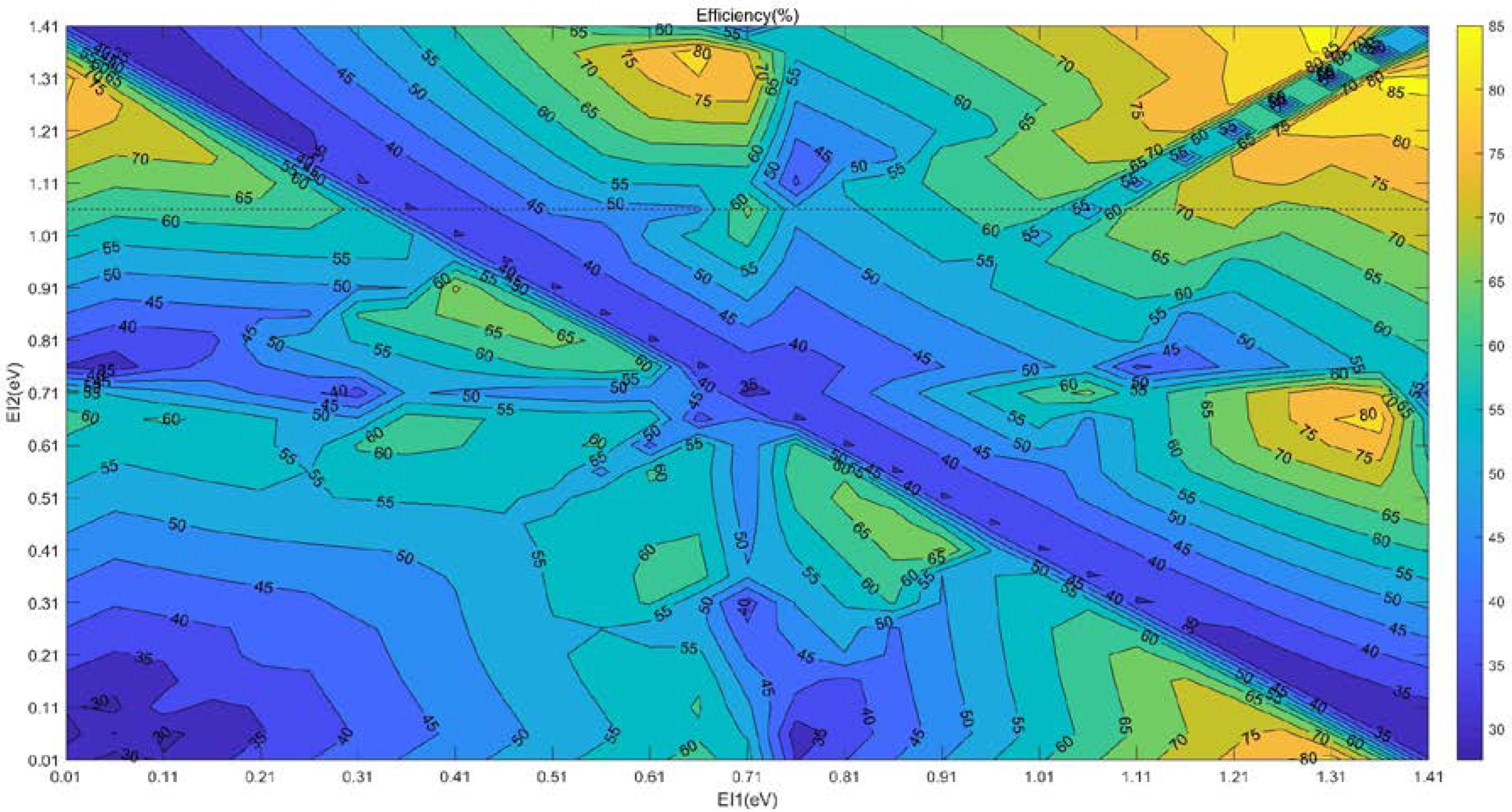
First, the calculation of the dual-intermediate-band solar cell is shown in Figure 3, where the EI1 (EI2) represents the space between the first (second) intermediate band and the VB. The efficiency clearly shows a flawless symmetrical distribution along the diagonal line EI1 = EI2 (it appears to be different because of the aspect ratio). When the positions of the dual intermediate bands are switched, both the absorption spectrum and quasi-Fermi levels associated with its own radiation are uniform, and the efficiency is also identical.
When EI1 = 1.31 eV and EI2 = 1.41 eV (which are interchangeable), the efficiency reaches the maximum value of 86.5%. If EI1 is equal to EI2, the dual intermediate bands degrade into a single IB; so, the diagonal line represents a single-intermediate-band solar cell with a maximum efficiency of 54.3% and EI1 = EI2 = 0.96 eV. The maximum efficiency is close to the limiting efficiency of 63.2% (EG = 1.95 eV and EI1 = 1.24 eV, but it is EG = 1.424 eV in this paper) [3,7]. In most areas of Figure 3, especially in the upper right area, the efficiency is higher than that of a solar cell with a single intermediate band.
For the reverse diagonal line L (EI2 = 1.42 eV − EI1, connected to the point EI1 = 0.01 eV, EI2 = 1.41 eV, and the point EI1 = 1.41 eV and EI2 = 0.01 eV) in Figure 3, the efficiency is about 35% in L, as well as all the points around it, which are low values in the entire graph. To understand why this is, each of points with small fluctuations near L can be defined as:
EI1 + EI2 + ∆ = 1.424 eV
where ∆ is a minimal value that can be positive or negative. The following analysis is performed with ∆ > 0 and EI2 > EI1+ ∆; in this way, with E3 = 1.424 eV − EI1 = EI2 + ∆ and E6 = 1.424 eV − EI2 = EI1 + ∆ combined with Equation (2), it is easy to solve for Equation (10):
The energy range is only ∆ for G2 and G4, while the energy range is larger for G3 and G6, resulting in G2 + G4 << G3 + G6. However, Equation (1) or Equation (6) is strict: the solar cell must convert the energy into a lower value; that is, G2 + G4 must be used as the lowest absorption value, and the total efficiency must be calculated by adding the G1 process. The spectral absorption of the dual intermediate bands is very small; so, the solar cell has similar characteristics to a GaAs solar cell without any intermediate band and utilizes most of the photons that transport electrons from the VB to the CB.
The above calculations are based on GaAs host materials, and all the possibilities are considered when GaAs is inserted into the dual intermediate bands. To achieve IBSC in experiments, the current IBSC uses mainly QDs (QD-IBSC), which always apply the Stranski–Krastanow (SK) growth mode in hetero-epitaxially mismatched systems and then a self-assembled InAs QDs island structure is formed on the GaAs surface due to strain [18]. By combining the previous calculations, it can be shown that the ternary alloy InxGa1−xAs QDs are used as the second intermediate band in the InAs/GaAs QDs system. The bandgap of the normal InAs material is 0.36 eV; however, due to the three-dimensional quantum confinement effect of QDs, the continuous bands show atom-like discrete energy levels (where the ground state is similar to s, and the excited state is similar to p). For an InAs/GaAs QDs system, the energy-level space between the ground-state electrons and holes in InAs QDs is 1.06 eV [21,22], and the bandgap becomes 0.7 eV [17]. If the VB is assumed to be continuous at both the QDs and the GaAs, the ground state in the InAs QDs valence band will be aligned with the GaAs valence band edge (∆EV = 0) [13,23]. In this way, the ground state in the CB of InAs QDs can be approximated as the first intermediate band, that is, the position 1.06 eV above the VB of the entire device. The same treatment can be performed for InxGa1−xAs QDs as the second intermediate band, the band diagram of which is shown in Figure 4. The density of the QDs is high enough to improve absorption coefficient, the carriers’ transfer is perfect, and the QDs have no defects. Combined with our calculation, the analyzation can be performed.
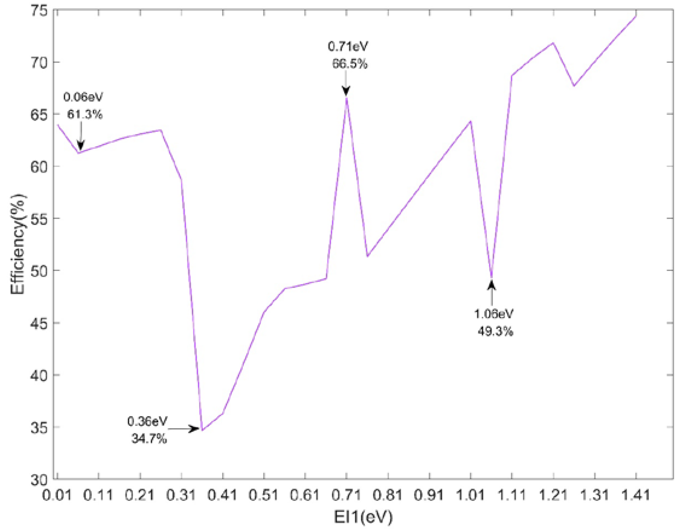
In Figure 3, in the case of EI2 = 1.06 eV, we extract the efficiency of all points from 0.01 eV to 1.41 eV for EI1, as shown in Figure 5 (all the points on the black dotted line in Figure 3).
The maximum efficiency is 74.4% when EI1 is 1.41 eV. For InxGa1−xAs QDs, the bandgap changes with composition because the energy-level space for the QD increases when its size is reduced [24]. If the size of InxGa1−xAs QDs is assumed to be the same as InAs QDs, then the ground-state energy levels of electrons and holes are considered to be relatively unchanged relative to the edge of the QD’s CB and VB. Therefore, the energy-level space between the ground-state electrons and holes is mainly due to the change in the bandgap. When the ground-state energy-level space of InxGa1-xAs changes from 1.06 eV of InAs (x = 1) to 1.41 eV, this indicates that the bandgap has increased by 0.35 eV, and the bandgap of InxGa1−xAs QDs is 0.7 eV + 0.35 eV = 1.05 eV, assuming that the bandgap between QDs and normal materials is fixed in proportion; that is, 0.7 eV/0.36 eV = 1.94. For InxGa1−xAs QDs, when its bandgap is 1.05 eV, the corresponding bandgap of the normal material is 1.05 eV/1.94 = 0.54 eV. According to Equation (11), the bandgap Eg of InxGa1-xAs varies with the composition [25]:
Eg = 0.36x + 1.42(1 − x) − 0.479x(1 − x)
Through these rough analyses and calculations, we can determine that the In component is 0.75, which means that the QD-IBSC for InAs/GaAs/InxGa1−xAs device can reach maximum efficiency of 74.4% through the use of In0.75Ga0.25As QDs.
The analysis of several feature points is given below for the four arrow points in Figure 5: A (0.06 eV, 61.3%), B (0.36 eV, 34.7%), C (0.71 eV, 66.5%), and D (1.06 eV, 49.3%). Point B has the lowest efficiency; it is not difficult to show this result when we consider the previous discussion about the L line. For point C, E2 = 0.71 eV, E3 = 0.714 eV, E4 = 1.06 eV, E6 = 0.364 eV, and its absorption cut-off energy is E5 = 0.35 eV, which is much larger than the cut-off energy of point A, 0.06 eV, but its efficiency is higher than that of point A. This phenomenon seems to contradict the intention of inserting the intermediate band, but this is explained in the next paragraph. For point D, E2 = E4 = 1.06 eV, E3 = E6 = 0.364 eV, and E5 becomes 0 eV; the dual intermediate bands degrade into a single IB and then the efficiency reaches a lower value of 49.3%.
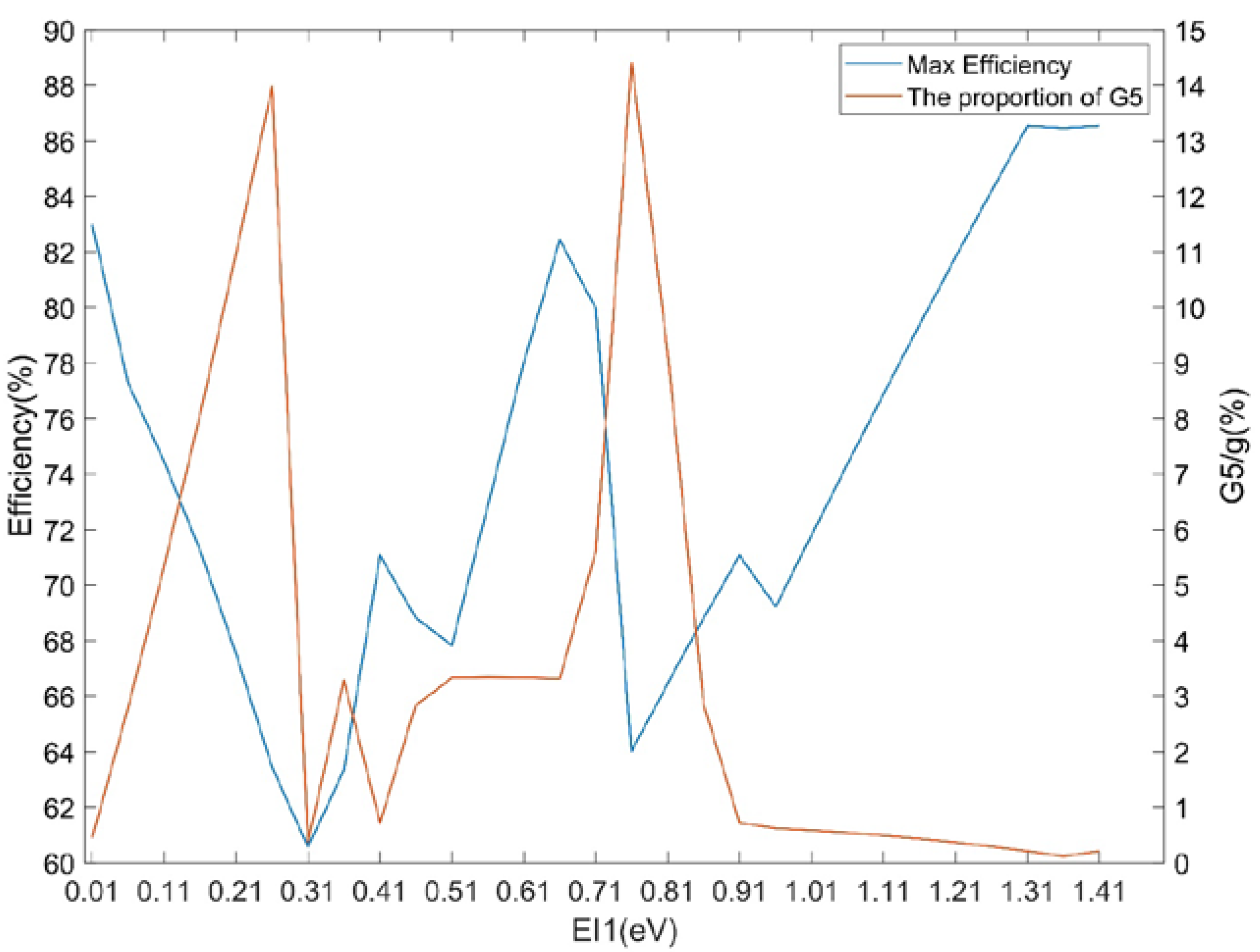
Next, EI1 is changed from 0.01 eV to 1.41 eV for a specific EI1, and the point is drawn that maximizes the efficiency in a series of EI2 (EI1 and EI2 are symmetrical in Figure 3, and changing EI2 is also permitted). These conditions allow for the process of dividing G5 by the total number of absorption photons g (not the net photons Ntotal), as shown in Figure 6.
An interesting phenomenon is that the G5/g and the maximum efficiency generally show an opposite trend. At its low efficiency point, the G5/g is large. The possible reason for this can be seen in Figure 2; the solar cell involves three different quantum efficiencies (QEs) for absorption. In the first process, the G1 absorbs a photon that is larger than the bandgap in order to generate a photocurrent with a QE of 100%. In the second process, if the G2, G3, G4, and G6 are involved, the electrons of the VB need two photons to arrive at the CB before the photocurrent generates; so, its QE is 50%. In the last transition G5 between the dual intermediate bands, an electron for the VB acquires three photons to generate at least a photocurrent, and its QE is 33.3%. Although the G5 process actually exists and cannot be eliminated, its optical–electrical conversion leads to more situations that satisfy the constraints of Equation (1) or Equation (6), which may be helpful in improving efficiency. However, it is unfortunate that the low QE eventually decreases the efficiency because G5 fails to utilize photons directly and efficiently. This discussion only pertains to devices with the same number of energy bands, and the greater the proportion of the first process the better. However, if compared with the structure with different numbers of energy bands, for example, a conventional solar cell, it only includes the process where the QE is 100%; on the other hand, the efficiency of the IBSC includes an additional process where the QE = 50%, but the IBSC is more efficient than a solar cell without an intermediate band. In other words, more intermediate bands include more QEs, and the minimum value of QE further reduces, but it is beneficial for multiple intermediate bands to broaden the long-wave absorption of the solar spectrum, and, thus, the theoretical efficiency increases rather than decreases.
Therefore, the G5 process may be the reason why point C is more efficient than point A. The absorption ranges of G5 at point A and point C are:
As discussed above, the G5 process fails to contribute a photocurrent directly to the CB. The larger the proportion of the G5, the worse the impact on the efficiency, which causes point A to be lower than point C.
Furthermore, combining the results shown in Figure 2 and Figure 4 indicates that a QD’s energy level is discrete, which is not conducive to electron transitions. To form two quasi-continuous intermediate bands, QDs must be uniform and dense so that electrons’ wave functions can overlap in barrier, and it is helpful to improve the absorption coefficient. For carrier transfer and collect, doping Si into QDs is helpful to fill the trap states and nonradiative centers and offer electrons to the IB [18]. At the same time, the G5 process is inevitable, as mentioned above, and its low QE also decreases the high-efficiency conversion. When ensuring the high density of QDs, it is necessary to design dual intermediate bands in a reasonable way and appropriately reduce the proportion of G5, which is advantageous for solar cells with dual intermediate bands.
4. Conclusions
In summary, this article shows that, based on the GaAs material, the maximum efficiency can reach 86.5% when the dual intermediate bands are above the VB with EI1 = 1.31 eV and EI2 = 1.41 eV. The solar cell with dual intermediate bands successfully extends the spectral absorption and, thus, increases the photocurrent compared with the solar cell with a single intermediate band, and the efficiency of the solar cell with dual intermediate bands was further increased. Then, on the basis of theoretical calculation of the QD-IBSC, the solar cell with InAs/GaAs/InxGa1−xAs quantum-dot dual intermediate bands is discussed in detail; the maximum efficiency is 74.4% when In0.75Ga0.25As QDs are used as an intermediate band. To create a high-performance solar cell with dual intermediate bands, the process of G5 is also worth noting. It is important to design the dual intermediate bands in a precise way when the high density of QDs grows.
Author Contributions
Conceptualization, S.W. (Shenglin Wang) and X.Y.; methodology, S.W. (Shenglin Wang) and X.Y.; software, S.W. (Shenglin Wang); validation, S.W. (Shenglin Wang) and X.Y.; formal analysis, S.W. (Shenglin Wang) and X.Y.; investigation, S.W. (Shenglin Wang), S.W. (Shuai Wang), H.W. (Haomiao Wang), and H.W. (Hong Wang); resources, T.Y.; data curation, S.W. (Shenglin Wang); writing—original draft preparation, S.W. (Shenglin Wang); writing—review and editing, S.W. (Shenglin Wang), X.Y., H.C., Z.L., and L.M.; visualization, S.W. (Shenglin Wang); supervision, T.Y. and X.Y.; project administration, T.Y. and X.Y.; funding acquisition, T.Y. and X.Y. All authors have read and agreed to the published version of the manuscript.
Funding
This research was funded by the National Key Research and Development Program of China (no. 2019YFB1503601) and the National Natural Science Foundation of China (nos. 62035012, 62074143, and 62004191).
Institutional Review Board Statement
Not applicable.
Informed Consent Statement
Not applicable.
Data Availability Statement
Not applicable.
Acknowledgments
The authors express their appreciation to the anonymous reviewers for their valuable suggestions.
Conflicts of Interest
The authors declare no conflict of interest.
References
Shockley, W.; Queisser, H.J. Detailed and Balance Limit of Efficience of p-n Junction Solar Cells. J. Appl. Phys.1961, 32, 510–519. [Google Scholar] [CrossRef]
Ariugo, G.L.; Martí, A. Absolute limiting efficiencies for photovoltaic energy conversion. Sol. Energy Mater. Sol. Cells1994, 94, 213–240. [Google Scholar]
Luque, A.; Martí, A. Increasing the efficiency of ideal solar cells by photon induced transitions at intermediate levels. Phys. Rev. Lett.1997, 76, 5014–5017. [Google Scholar] [CrossRef]
Green, M.A. Third generation photovoltaics: Ultra-high conversion efficiency at low cost. Prog. Photovolt. Res. Appl.2001, 9, 123–135. [Google Scholar] [CrossRef]
Ratner, M. Third Generation Photovoltaics: Advanced Solar Energy Conversion. Phys. Today2004, 57, 71–72. [Google Scholar] [CrossRef] [Green Version]
Luque, A.; Martí, A.; Stanley, C. Understanding intermediate-band solar cell. Nat. Photonics2012, 6, 146–152. [Google Scholar] [CrossRef] [Green Version]
Sahoo, G.S.; Mishra, G.P. Use of ratchet band in a quantum dot embedded intermediate band solar cell to enrich the photo response. Mater. Lett.2018, 218, 139–141. [Google Scholar] [CrossRef]
Luque, A.; Martí, A. Photovoltaics: Towards the intermediate band. Nat. Photonics2011, 5, 137–138. [Google Scholar] [CrossRef]
Lopez, N.; Reichertz, L.A.; Yu, K.M.; Campman, K.; Walukiewicz, W. Engineering the Electronic Band Structure for Multiband Solar Cells. Phys. Rev. Lett.2011, 106, 028701. [Google Scholar] [CrossRef] [PubMed]
Martí, A.; Cuadra, L.; Luque, A. Quantum dot intermediate band solar cell. In Proceedings of the Conference Record of the Twenty-Eighth IEEE Photovoltaic Sepecialists Conference-2000, Anchorage, AK, USA, 15–22 September 2000; pp. 940–943. [Google Scholar]
Tomic, S.; Jones, T.S.; Harrison, N.M. Absorption characteristics of a quantum dot array induced intermediate band: Implications for solar cell design. Appl. Phys. Lett.2008, 93, 263105. [Google Scholar] [CrossRef] [Green Version]
Sugaya, T.; Amano, T.; Mori, M.; Niki, S. Miniband formation in InGaAs quantum dot superlattice. Appl. Phys. Lett.2010, 97, 043112. [Google Scholar] [CrossRef]
Luque, A.; Martí, A.; Stanley, C.; López, N.; Cuadra, L.; Zhou, D.; Pearson, J.L.; McKee, A. General equivalent circuit for intermediate band devices: Potentials, currents and electroluminescence. J. Appl. Phys.2004, 96, 903–909. [Google Scholar] [CrossRef]
Antolin, E.; Martí, A.; Farmer, C.D.; Linares, P.G.; Hernández, E.; Sánchez, A.M.; Ben, T.; Molina, S.I.; Stanley, C.R.; Luque, A. Reducing carrier escape in the InAs/GaAs quantum dot intermediate band solar cell. J. Appl. Phys.2010, 108, 064513. [Google Scholar] [CrossRef] [Green Version]
Yang, X.G.; Wang, K.F.; Gu, Y.X.; Ni, H.; Wang, X.; Yang, T.; Wang, Z. Improved efficiency of InAs/GaAs quantum dots solar cells by Si-doping. Sol. Energy Mater. Sol. Cells2013, 113, 144–147. [Google Scholar] [CrossRef]
Naito, S.; Yoshida, K.; Miyashita, N.; Tamaki, R.; Hoshii, T.; Okada, Y. Effect of Si doping and sunlight concentration on the performance of InAs/GaAs quantum dot solar cells. J. Photonics Energy2017, 7, 025505. [Google Scholar] [CrossRef] [Green Version]
Zhu, M.F.; Xiong, S.Z. Basic and Application of Solar Cell; Science Press: Beijing, China, 2009; pp. 578–580. [Google Scholar]
Murata, T.; Asahi, S.; Sanguinetti, S.; Kita, T. Infrared photodetector sensitized by InAs quantum dots embedded near an Al0.3Ga0.7As/GaAs heterointerface. Sci. Rep.2020, 10, 11628. [Google Scholar] [CrossRef] [PubMed]
Zhu, Y.; Asahi, S.; Watanabe, K.; Miyashita, N.; Okada, Y.; Kita, T. Two-step excitation induced photovoltaic properties in an InAs quantum dot-in-well intermediate-band solar cell. J. Appl. Phys.2021, 129, 074503. [Google Scholar] [CrossRef]
Martí, A.; Cuadra, L.; Luque, A. Partial Filling of a Quantum Dot Intermediate Band for Solar Cells. IEEE Trans. Electron Devices2001, 48, 2394–2399. [Google Scholar] [CrossRef]
Fafrad, S.; Wasilewski, Z.R.; Allen, C.N.; Picard, D.; Spanner, M.; McCaffrey, J.P.; Piva, P.G. Manipulating the energy levels of semiconductor quantum dots. Phys. Rev. B1999, 59, 15368. [Google Scholar] [CrossRef] [Green Version]
Dong-Su, K.; Forrest, S.R.; Lange, M.J.; Cohen, M.J.; Paff, R.J. Study of InxGa1-xAs/InAsyP1-y structures lattice mismatched to InP substrates. J. Appl. Phys.1996, 80, 6229–6234. [Google Scholar]
Figure 1.
Simple structure of dual-intermediate-band solar cell.
Figure 1.
Simple structure of dual-intermediate-band solar cell.
Figure 2.
Solar cell with energy bands and transitions of dual intermediate bands. GaAs is a barrier material, and IB and IB2 are the dual intermediate bands.
Figure 2.
Solar cell with energy bands and transitions of dual intermediate bands. GaAs is a barrier material, and IB and IB2 are the dual intermediate bands.
Figure 3.
Efficiency contour plot of dual intermediate bands. The right color gradient bar shows the efficiency.
Figure 3.
Efficiency contour plot of dual intermediate bands. The right color gradient bar shows the efficiency.
Figure 4.
Dual intermediate band structure for the InAs/GaAs/InxGa1−xAs QDs system.
Figure 4.
Dual intermediate band structure for the InAs/GaAs/InxGa1−xAs QDs system.
Figure 5.
Efficiency for EI2 = 1.06 eV, where EI1 changes from 0.01 eV to 1.41 eV.
Figure 5.
Efficiency for EI2 = 1.06 eV, where EI1 changes from 0.01 eV to 1.41 eV.
Figure 6.
Maximum efficiency and the value of G5/g for a certain EI1 when EI2 changes from 0.01 eV to 1.41 eV. Only the point of maximum efficiency is shown.
Figure 6.
Maximum efficiency and the value of G5/g for a certain EI1 when EI2 changes from 0.01 eV to 1.41 eV. Only the point of maximum efficiency is shown.
Publisher’s Note: MDPI stays neutral with regard to jurisdictional claims in published maps and institutional affiliations.
Wang, S.; Yang, X.; Chai, H.; Lv, Z.; Wang, S.; Wang, H.; Wang, H.; Meng, L.; Yang, T.
Detailed Balance-Limiting Efficiency of Solar Cells with Dual Intermediate Bands Based on InAs/InGaAs Quantum Dots. Photonics2022, 9, 290.
https://doi.org/10.3390/photonics9050290
AMA Style
Wang S, Yang X, Chai H, Lv Z, Wang S, Wang H, Wang H, Meng L, Yang T.
Detailed Balance-Limiting Efficiency of Solar Cells with Dual Intermediate Bands Based on InAs/InGaAs Quantum Dots. Photonics. 2022; 9(5):290.
https://doi.org/10.3390/photonics9050290
Chicago/Turabian Style
Wang, Shenglin, Xiaoguang Yang, Hongyu Chai, Zunren Lv, Shuai Wang, Haomiao Wang, Hong Wang, Lei Meng, and Tao Yang.
2022. "Detailed Balance-Limiting Efficiency of Solar Cells with Dual Intermediate Bands Based on InAs/InGaAs Quantum Dots" Photonics 9, no. 5: 290.
https://doi.org/10.3390/photonics9050290
Note that from the first issue of 2016, this journal uses article numbers instead of page numbers. See further details here.
Article Metrics
No
No
Article Access Statistics
For more information on the journal statistics, click here.
Multiple requests from the same IP address are counted as one view.
Wang, S.; Yang, X.; Chai, H.; Lv, Z.; Wang, S.; Wang, H.; Wang, H.; Meng, L.; Yang, T.
Detailed Balance-Limiting Efficiency of Solar Cells with Dual Intermediate Bands Based on InAs/InGaAs Quantum Dots. Photonics2022, 9, 290.
https://doi.org/10.3390/photonics9050290
AMA Style
Wang S, Yang X, Chai H, Lv Z, Wang S, Wang H, Wang H, Meng L, Yang T.
Detailed Balance-Limiting Efficiency of Solar Cells with Dual Intermediate Bands Based on InAs/InGaAs Quantum Dots. Photonics. 2022; 9(5):290.
https://doi.org/10.3390/photonics9050290
Chicago/Turabian Style
Wang, Shenglin, Xiaoguang Yang, Hongyu Chai, Zunren Lv, Shuai Wang, Haomiao Wang, Hong Wang, Lei Meng, and Tao Yang.
2022. "Detailed Balance-Limiting Efficiency of Solar Cells with Dual Intermediate Bands Based on InAs/InGaAs Quantum Dots" Photonics 9, no. 5: 290.
https://doi.org/10.3390/photonics9050290
Note that from the first issue of 2016, this journal uses article numbers instead of page numbers. See further details here.

 ,
, 


