Deep Neural Network Based Reconciliation for CV-QKD

Abstract

High-speed reconciliation is indispensable for supporting the continuous-variable quantum key distribution (CV-QKD) system to generate the secure key in real-time. However, the error correction process’s high complexity and low processing speed limit the reconciliation speed. Therefore, reconciliation has also become the bottleneck of system performance. In this paper, we proposed a high-speed reconciliation scheme that uses the deep neural network to optimize the decoding process of the low-density parity-check (LDPC) code. We first introduced a network structure of decoding implementation based on the deep neural network, which can be applied to decoding algorithms of parallel strategy and significantly reduce the decoding complexity. Subsequently, we proposed two improved decoding algorithms based on this structure, named linear fitting algorithm and deep neural network-assisted decoding algorithm. Finally, we introduced a high-speed reconciliation scheme based on the CPU-GPU hybrid platform. Simulation results show that the proposed reconciliation scheme reduces the complexity and enables us to realize the high-speed CV-QKD system. Furthermore, the improved decoding algorithm can also reduce the FER, thereby increasing the secret key rate.

1. Introduction

Quantum key distribution (QKD) [1] enables two remote communication terminals, commonly called Alice and Bob, to share the unconditional secure key, even in the presence of eavesdropper Eve. In recent decades, QKD has been widely studied and has achieved remarkable progress because it ensures the confidentiality and security of the communication process [2]. According to the coding dimension of transmitted information, QKD could be divided into the discrete variable QKD (DV-QKD) [3,4] and the continuous-variable QKD (CV-QKD) [5,6,7,8]. The former encodes information in discrete variables, such as the polarization or phase of a single photon, and it has relatively mature development, coupled with a farther communication distance. The latter encodes information in continuous variables, such as the regular components of coherent states, and it achieves a higher secret key rate at a close distance. Due to the easier preparation and measurement of quantum states, CV-QKD has a higher practical value and has been extensively studied.

Reconciliation [9,10,11] plays an indispensable role in CV-QKD, and its performance is the main factor of system performance [12]. In reconciliation, we first perform related processing on the original key. Then, we use mature channel error correction technology to correct the inconsistent data bits between the two communication terminals, thereby obtaining the secure key. We need to use an error correction code near Shannon channel capacity, usually the low-density parity-check (LDPC) code [2,13,14], to realize efficient reconciliation. However, under the condition of extremely low signal-to-noise ratio (SNR), better error correction performance is usually accompanied by higher algorithm complexity. Therefore, the high complexity and low processing speed of decoding implementation still limit the reconciliation performance.

Belief propagation (BP) [15,16,17] and layered belief propagation (LBP) [18,19] are two main LDPC decoding algorithms in reconciliation. In [20], Dakai Lin proposed a well-structured decoding scheme that reached a reconciliation speed of 25 Mb/s. Simplified algorithms in classic communication systems effectively reduce the complexity of message iteration but also cause performance degradation and cannot be applied to CV-QKD systems [21]. Deep learning [22] can obtain more significant performance improvements than traditional methods in many fields, and we can apply it to the research of channel decoding. In [23], the BP algorithm is described as the forward neural network. Results prove that the combination of deep neural network and BP decoding algorithm can improve the decoding performance. In [24], Fei Liang combines traditional BP decoder and convolutional neural network (CNN) to improve error correction performance. In [25], Lugosch proposes the neural offset min-sum (NOMS) decoding algorithm conducive to hardware implementation. Although these neural network decoding algorithms improve performance to a certain extent, they also cause additional complexity. Therefore, they are not well suited for reconciliation.

In this paper, we proposed a high-speed reconciliation scheme by using the deep neural network to optimize the performance of the LDPC decoding process. First, we introduced the network structure of the decoding implementation. Then, we proposed some improved decoding algorithms based on the network structure. Finally, we proposed a high-speed reconciliation scheme based on the CPU-GPU hybrid platform. Simulation results show that the proposed method effectively reduces the decoding complexity and enables us to achieve high-speed decoding of 26.7 Mbits/s. Moreover, some improved algorithms can slightly increase the secret key rate.

The rest of this paper is organized as follows. First, we introduced some preliminaries in Section 2. Then, in Section 3, we proposed a high-speed reconciliation scheme. We provided the network training strategy and related simulation results of the proposed scheme in Section 4. Finally, conclusions and future works are drawn in Section 5.

2. Preliminaries

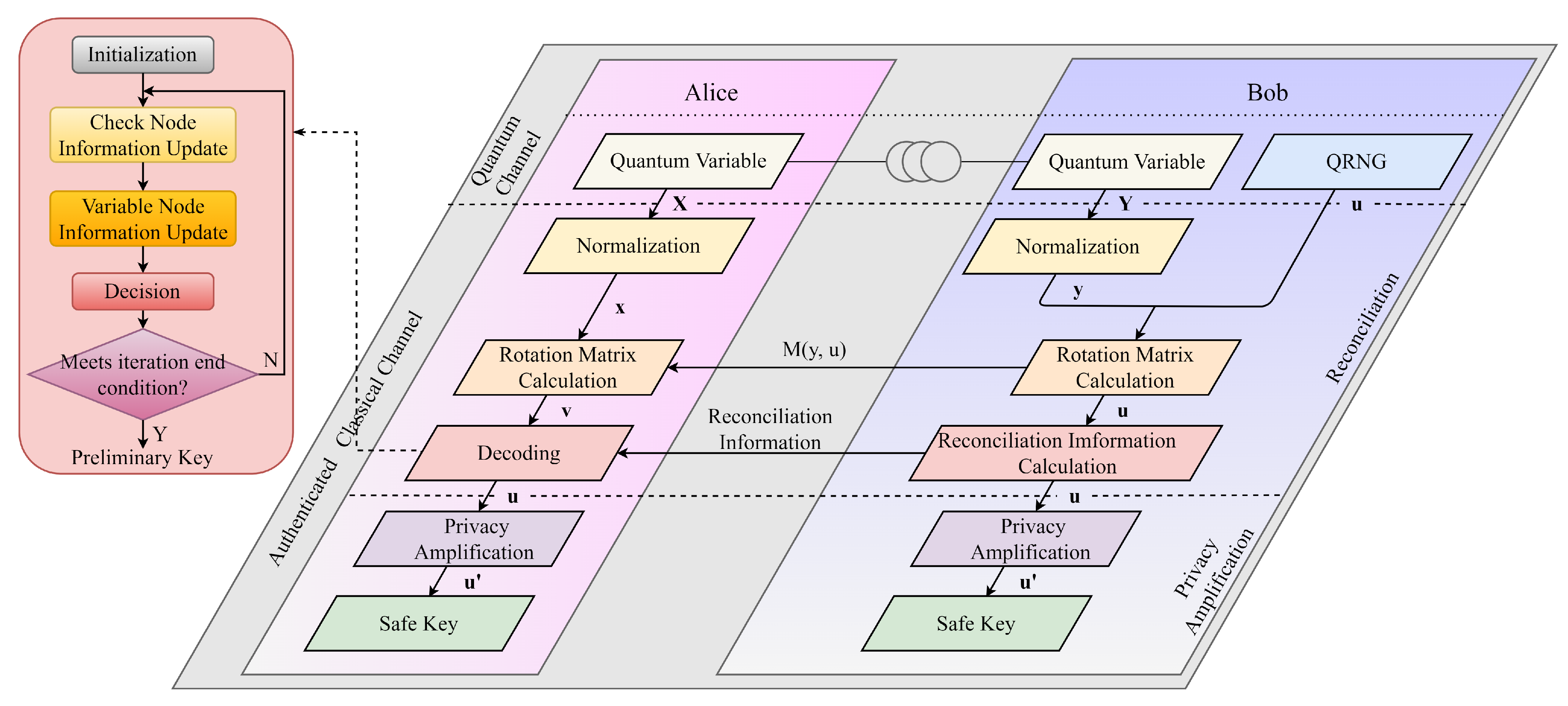
2.1. Brief Description of CV-QKD Post-Processing

Generally, in the Gaussian-modulated coherent CV-QKD system, when the transmitter Alice sends string X to the receiver Bob via the quantum channel, the detected string Y can only be a certain correlated with X, but not consistent, due to the influence of noise, channel loss, and even potential Eve in the quantum channel. According to the characteristics of the quantum channel, both X and Y are continuous variables that obey the Gaussian distribution [26], which can be expressed as

$$X\sim N\left(0,{\sigma }_x^2\right),Y\sim N\left(0,{\sigma }_y^2\right).$$

(1)

where ${\sigma }_y^2={\sigma }_x^2+{\sigma }_{\mathrm{e}}^2$, and ${\sigma }_{\mathrm{e}}^2$ is the noise variance of quantum channel.

In order to ensure that Alice and Bob can obtain the secure key, we need to post-process the original key (X and Y). Figure 1 shows the flow chart of post-processing. Post-processing mainly includes the reconciliation [9,10,11] and the privacy amplification [27,28,29], both performed on the authenticated classical channel, and Eve can obtain the information exchanged between two communication terminals.

Since information is carried on the continuous variables and cannot be corrected directly, it is usually necessary to convert them into discrete forms through reconciliation algorithms. Sign reconciliation [30] or slice reconciliation [10] is generally only suitable for the high SNR conditions. The theory proves that Gaussian variables that obey independent and identical distribution obey uniform distribution on the multi-dimensional sphere. Therefore, we can transform the reconciliation process into the error correction problem on the binary additive white Gaussian noise channel (BIAWGNC) through normalization and rotation mapping operations. This method is called the multi-dimensional reconciliation algorithm [31]. We can obtain high-performance reconciliation with the error correction code close to Shannon channel capacity, usually the LDPC code. Further, in order to achieve secure long-distance communication, we need to adopt the reverse reconciliation [32], that is, Alice complete error correction based on Bob’s reconciliation information, effectively avoiding the influence of Eve, overcoming the channel loss limitation of 3 dB, and significantly improving the security of the entire system.

Alice and Bob obtain the preliminary final key after the reconciliation process. However, since the information exchange is carried out on the public channel, Eve may infer the key information from these parts of reconciliation information. Therefore, one necessary step, named privacy amplification, usually deletes part of the information to ensure the security of the final key.

2.2. Reconciliation with LDPC Code

In simple terms, reconciliation is actually a process in which two legal terminals accomplish error correction through information exchange. LDPC code, designed by density evolution algorithm [33,34,35,36], is close to Shannon limit on the AWGN channel and achieves a higher decoding throughput [37,38,39], applying the BP algorithm, more precisely, the log-likelihood ratio BP (LLR-BP) algorithm. Since the LDPC code has excellent error correction performance, we apply it to reconciliation, significantly reducing the frame error rate (FER), increasing the secret key rate, and extending the secure communication distance.

Tanner graph is the graphical representation of check matrix of LDPC code [37,40,41], composed of check nodes $C_j$, variable nodes $V_i$, and connecting edges. Equation (2) shows a simple check matrix, and Figure 2 shows the corresponding Tanner graph and information transmission process.

$$H=\left[\begin{array}{cccccc}1\hfill & 1\hfill & 0\hfill & 1\hfill & 0\hfill & 0\hfill \\ 1\hfill & 0\hfill & 1\hfill & 0\hfill & 1\hfill & 0\hfill \\ 0\hfill & 1\hfill & 1\hfill & 0\hfill & 0\hfill & 1\hfill \end{array}\right]$$

(2)

We usually use circles to represent the variable nodes $V_i$ and squares to represent the check nodes $C_j$. In addition, if $H(i,j)$ is not 0, then $V_i$ is connected to $C_j$. Otherwise, they are not connected [42]. Messages are transmitted iteratively between check and variable nodes through the edges to achieve decoding. Let $L\left(P_i\right)$ be the log-likelihood ratio of the received message, k be the number of iterations, and the LLR-BP decoding algorithm is divided into the following steps:

• Step 1, initialization.

  $$L\left(q_{ij}^{\left(0\right)}\right)=L\left(P_i\right)=2y_i/{\sigma }^2,i=1,2\dots N.$$

  (3)

  where $y_i$ is the ith bit of the received message and ${\sigma }^2$ is the noise variance of the transmission channel.
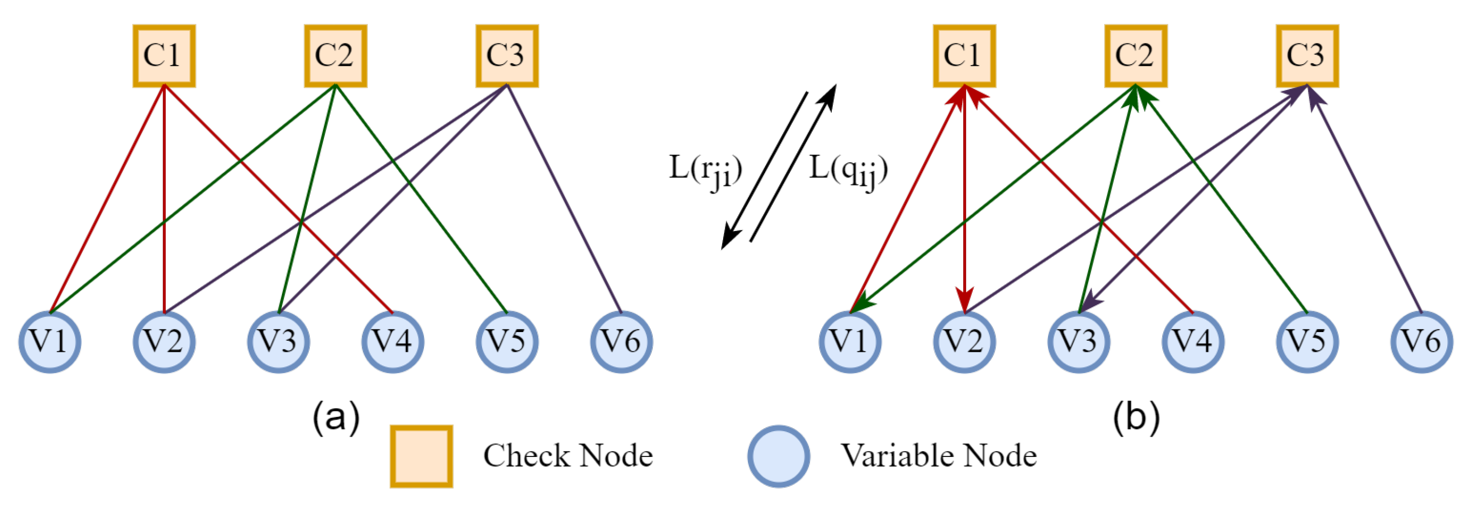
• Step 2, check nodes information update.

  $$L\left(r_{ji}^{\left(k\right)}\right)=2{tanh}^{-1}\left(\prod _{i^{\prime }\in C\left(j\right)\backslash i}tanh\left(L\left(q_{i^{\prime }j}^{(k-1)}\right)/2\right)\right).$$

  (4)

  where $L\left(r_{ji}\right)$ is the information transmitted by the check node $C_j$ to the variable node $V_i$. It is calculated based on the information from the set of all variable nodes connected to $C_j$, excluding the variable node $V_i$, and can be expressed as $i^{\prime }\in C\left(j\right)\backslash i$.
• Step 3, variable nodes information update.

  $$L\left(q_{ij}^{\left(k\right)}\right)=L\left(P_i\right)+\sum _{j^{\prime }\in C\left(i\right)\backslash j}L\left(r_{j^{\prime }i}^{\left(k\right)}\right).$$

  (5)

  where $L\left(q_{ij}\right)$ is the information transmitted by the variable node $V_i$ to the check node $C_j$. It is calculated based on the information from the set of all check nodes connected to $V_i$, excluding the check node $C_j$, and can be expressed as $j^{\prime }\in C\left(i\right)\backslash j$.
• Step 4, log-likelihood ratio of variable nodes update and decision.

  $$L\left(Q_i^{\left(k\right)}\right)=L\left(P_i\right)+\sum _{j^{\prime }\in C\left(i\right)}L\left(r_{j^{\prime }i}^{\left(k\right)}\right),{\widehat{y}}_i=\left\{\begin{array}{c}1,L\left(Q_i\right)\le 0\hfill \\ 0,L\left(Q_i\right)>0\hfill \end{array}.\right.$$

  (6)

  where ${\widehat{y}}_i$ is the ith bit of the decoded message. The iteration ends when k reaches the maximum number of iterations or $H·{\widehat{y}}^T=0$; otherwise, go back to Step 2.

3. High-Speed Multi-Dimensional Reconciliation

Speed and efficiency are two key technical parameters of reconciliation. The former has an important impact on the number of keys obtained by the system per unit time. Considering the system’s security, we need to realize real-time key generation. The latter directly affects the secret key rate [6,31,43] and secure communication distance of the system. The higher the value, the longer the transmission distance supported.

We adopt the reverse multi-dimensional reconciliation scheme with LDPC code in this paper. The specific process follows [31]: First, the original keys X and Y are normalized to obtain x and y separately. Second, Bob generates a spherical code u, calculates the rotation mapping relationship $M(y,u)$, which satisfies $M(y,u)y=u$, and sends $M(y,u)$ to Alice. Alice does the same rotation on x to obtain the noisy form v of u. Finally, Bob selects the appropriate LDPC code whose check matrix is H, uses u to calculate the syndrome $c_B$, which satisfies $c_B=H{u}^T$, and sends $c_B$ to Alice as the reconciliation information. Alice uses this information, v, and H to complete decoding and finally obtains the same binary bit u as Bob. Therefore, multi-dimensional reconciliation can be divided into reconciliation and error correction processes. The former has low computational complexity; the latter is the most important and the most complicated step. Our purpose is to use the powerful data processing capability of the deep neural network to optimize decoding performance, thereby increasing the reconciliation speed and improving the secret key rate.

3.1. Proposed Network Structure of Decoding Implementation

The LLR-BP algorithm is a message-passing algorithm, and its implementation directly corresponds to the Tanner graph. Fortunately, the Tanner graph is a natural network structure, and we can naturally think of a neural network with similar structures.

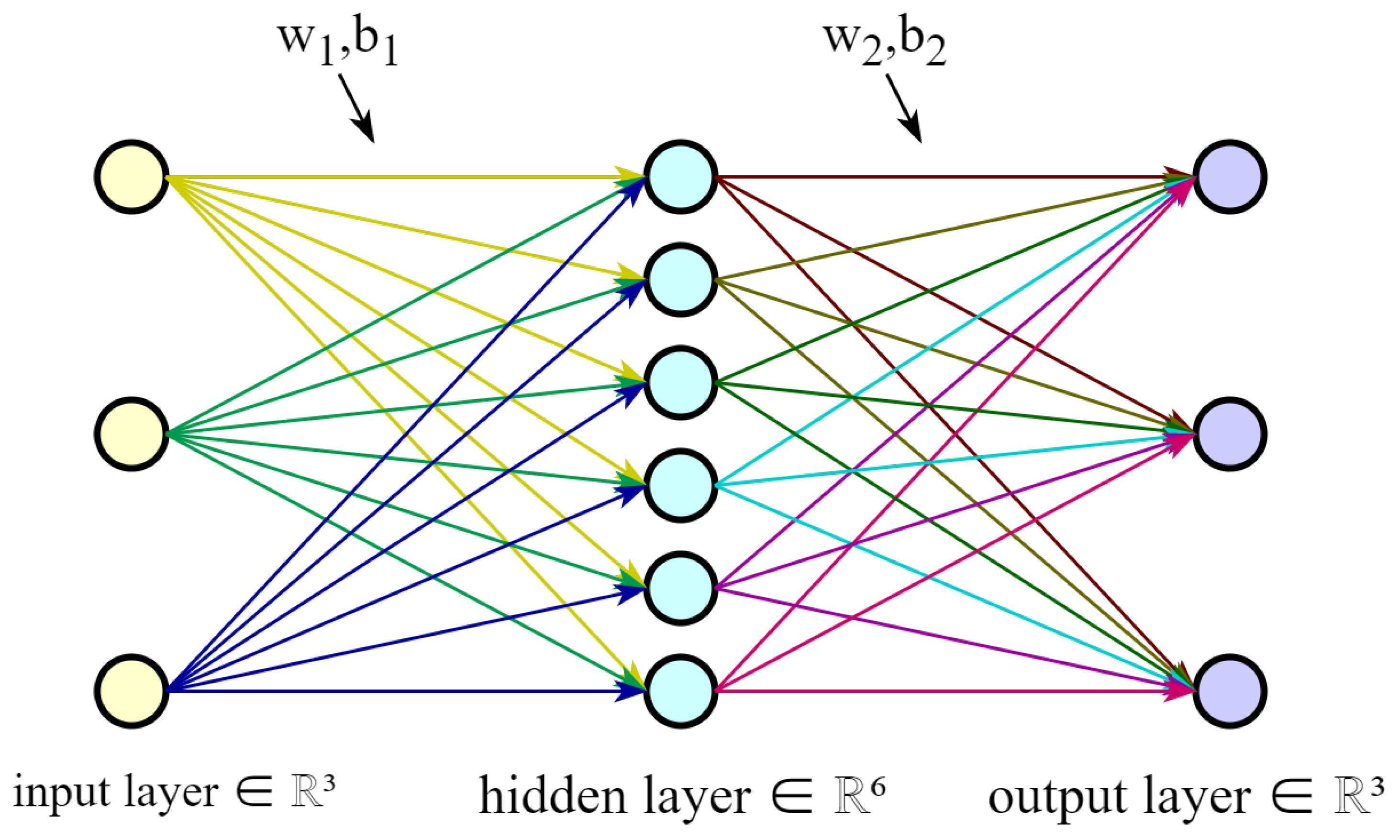
3.1.1. Multi-Layer Perceptron (MLP)

MLP is also called the artificial neural network (ANN) [44]. It includes an input layer, an output layer, and multiple hidden layers. Figure 3 shows the simplest MLP, a three-layer network structure with only one hidden layer.

As can be seen from the above figure, the two layers of MLP are fully connected, which means that neurons in different network layers are all connected. Denote the vector x represents the network’s input, so the output of the hidden layer is $f\left(w_{1}x+b_1\right)$. $w_1$ is the weight, $b_1$ is the bias, and f is the activation function, which commonly uses $sigmoid$ function or $tanh$ function.

$$f_{\mathrm{sigmoid}}\left(x\right)=\frac{1}{e^{-x}+1},f_{\tan \mathrm{h}}\left(x\right)=\frac{e^x-e^{-x}}{e^x+e^{-x}}.$$

(7)

If the activation function is not defined, the output of this layer is equal to $(w_{1}x+b_1)$. Therefore, the most critical elements of constructing a neural network include the dimensions of each network layer, the calculation formula of each neuron, the depth of the network, and the network connections between layers.

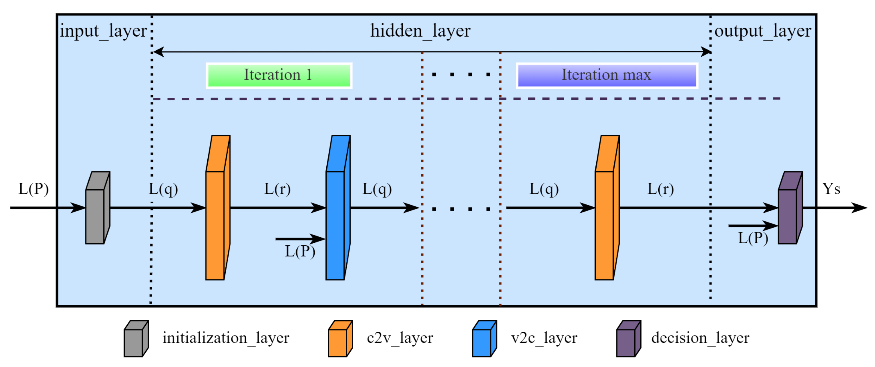
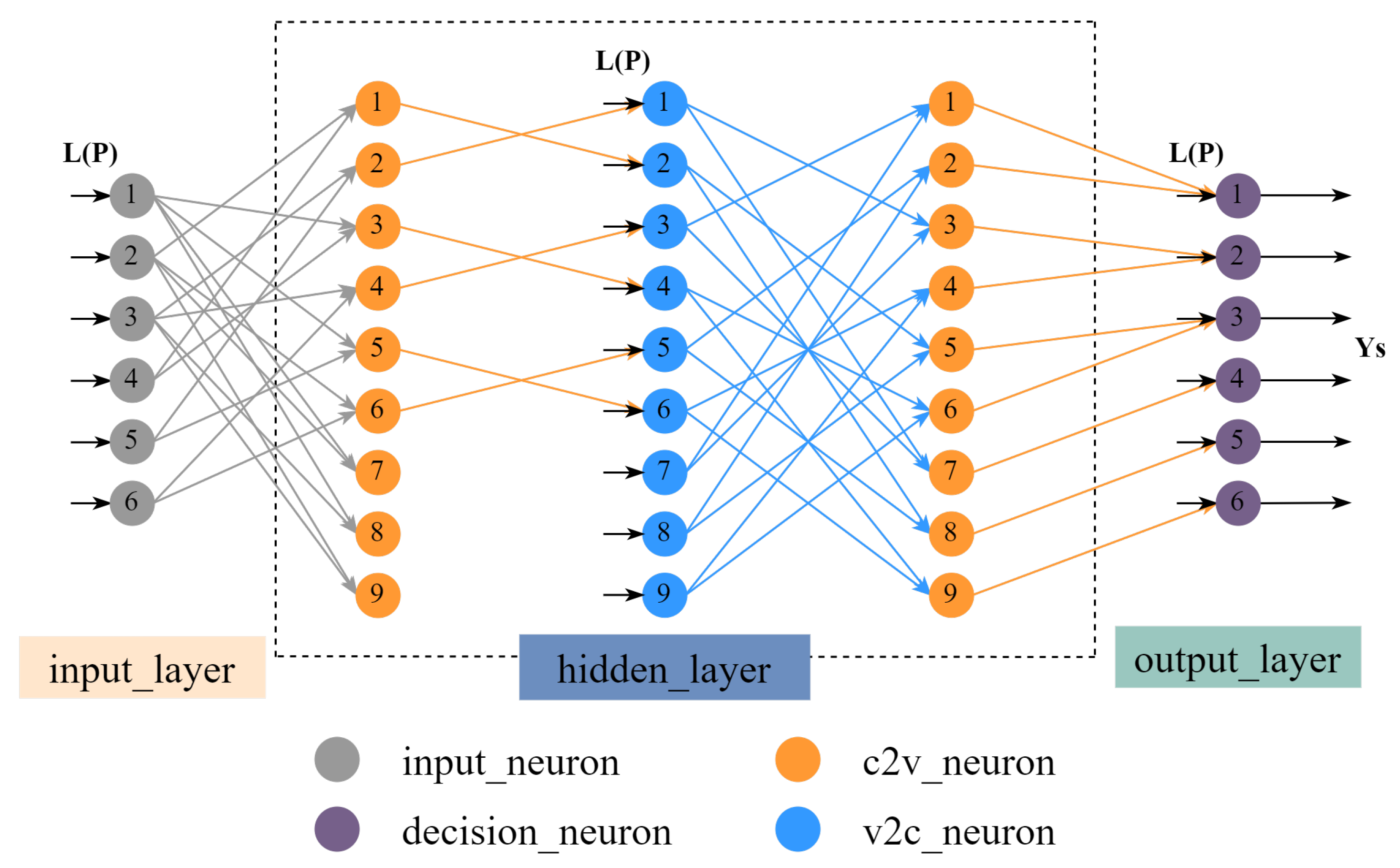
3.1.2. Proposed Decoding Network Structure

According to the content described in Section 2, the decoding performance of the LDPC code is mainly related to the following factors, e.g., the information update algorithm, the structure of the check matrix, the maximum number of iterations, etc. These factors also determine the network structure of the decoding implementation.

• The information update algorithm affects the error correction performance and determines the neurons’ specific connection mode between the network layers. Different from the fully connected network structure of MLP, our network connection depends on the information needed for the calculation of the neuron information. In other words, we only need to send the information needed in the calculation formula of the node to the node.
• The structure of the check matrix determines its maximum error correction capability. Furthermore, the number of columns determines the dimensions of the input and output layers, and the number of non-zero elements determines the dimensions of the hidden layer.
• The maximum number of iterations has a considerable influence on the error correction performance and determines the depth of the network. We can adjust the maximum number of iterations within a certain range to improve error correction performance. If the maximum number of iterations is set too small, the network depth is low, and the decoding success rate is low. On the contrary, if the maximum number of iterations is too large, it will cause excessive network depth and high time consumption.

Figure 4 shows the network structure of the decoding implementation. It is worth noting that the network structure we proposed does not wholly correspond to the traditional decoding iterative process. There are three reasons for this. (a) Under low SNR, decoding usually stops when the upper limit of the number of iterations is reached. (b) If the correct codeword has been obtained in a few iterations, the transmitted information has already converged at this time, and subsequent network propagation will not change its sign. (c) We also consider the training of the deep neural network decoding algorithm. In order to ensure that the training of the neural network can obtain the optimal parameters of the network, we need to adopt the most complex decoding conditions when training the network, that is, the decoding stops when the upper limit of the number of iterations is reached. Therefore, the entire network can be divided into one input layer, $(2I-1)$ hidden layers, and one output layer, where I is the maximum number of iterations. Assuming that the check matrix H is a $(M,\mathrm{N})$ matrix and the number of non-zero elements is E, the specific design of the three network layers is described as follows.

First, the input layer is composed of N neurons. This layer corresponds to the initialization process of decoding. Therefore, the input of this layer is the log-likelihood ratio (LLR) of the channel received information, and the output is the initial information of the variable nodes.

Then, the hidden layer is composed of E neurons. All iterations except the last iteration correspond to two hidden layers, named c2v_layer and v2c_layer. They calculate check and variable nodes information, respectively. The last iteration only includes one c2v_layer because it does not need to calculate variable node information. In the Tanner graph, the non-zero elements of the check matrix determine the connecting edge between the variable node and the check node. Drawing on this idea, we first sort the non-zero elements of the check matrix by column and then correspond each non-zero element to a neuron in the hidden layer. Therefore, the number of neurons in all hidden layers is E. In addition, there are already definite network connections between different layers instead of the fully connected structure of traditional neural networks. The reason is that these neurons only need the corresponding node information in the calculation formula. It should be noted that neither the input layer nor the hidden layer needs to define an activation function. We can directly calculate the corresponding value according to the LLR-BP decoding algorithm.

Finally, the output layer comprises N neurons and outputs the final decoded codeword. The activation function of this layer is defined as

$$\sigma \left(x\right)=\frac{1-sgn\left(x\right)}{2},sgn\left(x\right)=\left\{\begin{array}{c}-1,x<=0\\ 1,x>0\end{array}\right.$$

(8)

For clarity, we take Equation (2) as an example to illustrate using the check matrix to generate the corresponding network structure. First, we number the non-zero elements of the check matrix in column order.

$$\widehat{H}=\left[\begin{array}{cccccc}1\hfill & 3\hfill & 0\hfill & 7\hfill & 0\hfill & 0\hfill \\ 2\hfill & 0\hfill & 5\hfill & 0\hfill & 8\hfill & 0\hfill \\ 0\hfill & 4\hfill & 6\hfill & 0\hfill & 0\hfill & 9\hfill \end{array}\right]$$

(9)

Then, the non-zero elements correspond to the neurons in the hidden layer in order. Moreover, the connecting edge of the neuron is only the information needed for formula calculation. Figure 5 shows the network structure of the above matrix.

3.1.3. Advantages of Proposed Network Structure

Our method is to expand the iterative decoding process into a forward propagation network to reduce complexity, thereby speeding up the decoding process. Compared with the traditional decoding implementation, the decoding network structure has the following advantages.

• The node information of the traditional algorithm is transmitted in the form of a matrix with the same shape as the check matrix. The network structure we proposed expands the two-dimensional matrix into a one-dimensional vector, optimizes the storage structure of the check matrix, and saves a lot of storage space.
• We arrange the transmitted information in order, which makes the memory read and write orderly, so the time delay of data read and write is significantly reduced, improving the decoding speed.
• We have neglected the update of variable nodes with degree 1 in the network construction, reducing unnecessary operations of traditional decoding algorithms.
• The forward propagation network eliminates the need for multiple iterations of decoding. Without iteration, we input the channel message into the network and obtain the decoded codewords [45].
• Since the network is fully parallel, we can use powerful hardware, such as graphics processing unit (GPU) or field-programmable logic gate array (FPGA), to process multiple data at once.
• This network structure is suitable for decoding algorithms with parallel strategy, and training network parameters can also improve the decoding algorithm. All we need to do is adjust the neuron’s calculation formula.

3.2. Linear Fitting Decoding Algorithm

The LLR-BP decoding algorithm has excellent error correction performance, but its computational complexity is relatively high, especially the calculation of check node information. The main calculations in the formula are concentrated in $tanh\left(x\right)$ and $tan{h}^{-1}\left(x\right)$. We focus on simplifying complexity on $tanh\left(x\right)$ because $tan{h}^{-1}\left(x\right)$ is calculated only once.

Since $tanh\left(x\right)$ is an odd function and takes $y=\pm 1$ as the asymptote, we assume that the approximation function $F\left(x\right)$ has the following form,

$$F\left(x\right)=\left\{\begin{array}{cc}h\left(x\right),\hfill & x\in [0,+\infty )\hfill \\ -h(-x),\hfill & x\in (-\infty ,0)\hfill \end{array}\right..$$

(10)

where $h\left(x\right)$ has the following algebraic form,

$$h\left(x\right)=\frac{\left.\left.\left(\dots \left(a_{n}x+a_{n-1}\right)x+a_{n-2}\right)\dots \right)x+a_1\right)x}{\left.\left.\left(\dots \left(b_{n}x+b_{n-1}\right)x+b_{n-2}\right)\dots \right)x+b_1\right)x+b_0}.$$

(11)

where n is the highest power of the numerator (or denominator), and $a_n$ and $b_n$ are weight coefficients. Then, we can use the deep learning method to obtain the optimal weight coefficients. The sample label is $tanh\left(x\right)$, the network output is $F\left(x\right)$, and the training goal is to minimize the difference between the above two. We use the mean square error (MSE) loss function to train the network, which is defined as

$$\mathrm{MSE}=\frac{1}{m}\sum _{i=1}^m{[tanh\left(i\right)-F\left(i\right)]}^2.$$

(12)

where m is the number of samples.

Table 1. The MSE under different parameter settings.

n	MSE
3	6.133325138919856 × 10${}^{-7}$
4	1.2272255835313485 × 10${}^{-8}$
5	8.221156127182263 × 10${}^{-13}$

illustrates the MSE under different parameter settings.

3.3. Deep Neural Network-Assisted Decoder

The above method is to optimize the algorithm by reducing the complexity, and then we will introduce an algorithm to improve the error correction performance. We can increase the role of LLR information with a larger absolute value in information update because the larger the absolute value of the LLR, the greater the probability difference between 0 and 1, and the more reliable this LLR value is. On the contrary, we need to reduce the influence of this value in the decoding process. In short, our idea is to add a corresponding correction factor for each node information to adjust the reliability of the transmitted information, thereby increasing the convergence speed of the algorithm. Corresponding to the network structure, we add weight or bias to the network [23,25]. We can use the backpropagation algorithm to update the parameters in the network and realize the optimal design of the network. In this part, we first propose a general model of the simulation system based on the deep neural network-assisted decoder (DNNAD). Subsequently, we introduce the specific structure of the DNNAD.

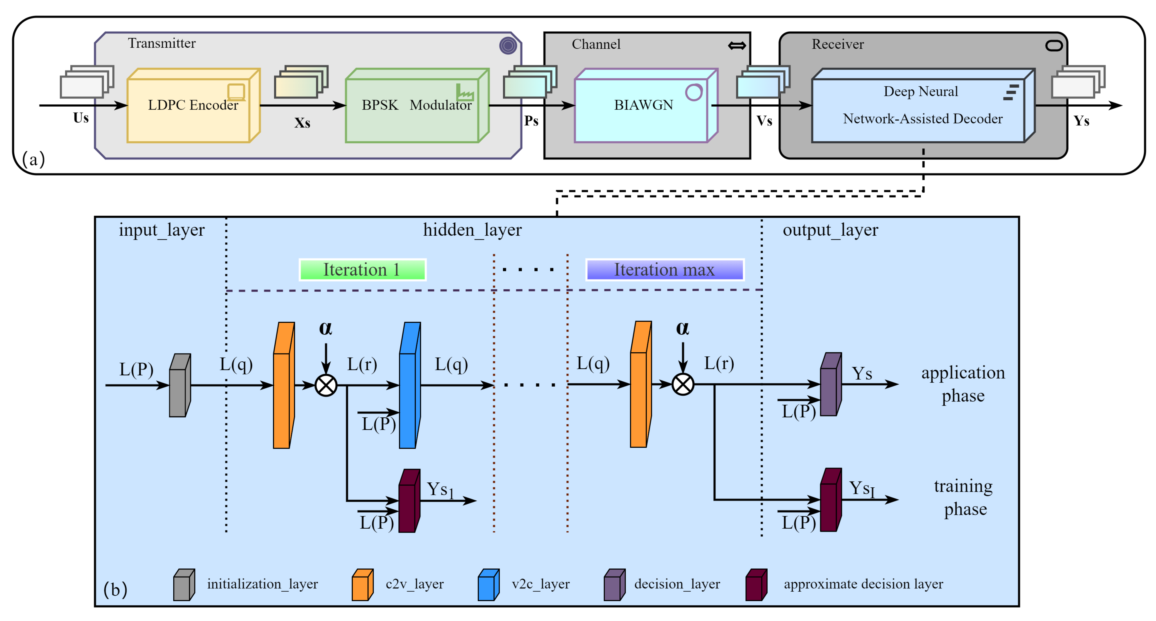
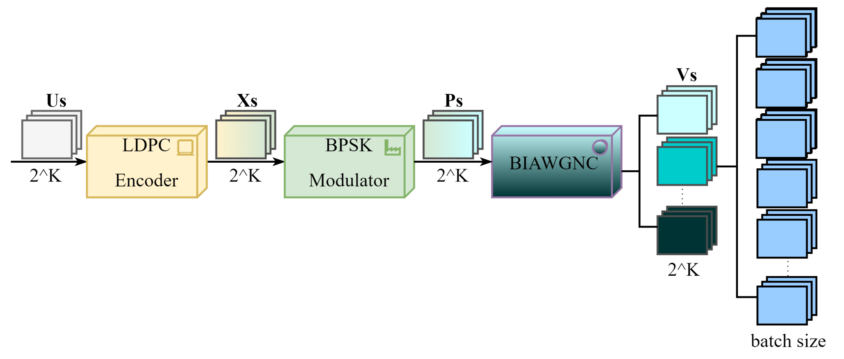
3.3.1. General Model of Simulation System

Since the data of the experiment system is not easy to obtain, we built this simulation system to obtain sample data for network training. All system parts are in parallel structure and can process multiple data simultaneously. Figure 6a shows the general model of the simulation system based on the DNNAD. We can easily obtain a large amount of sample data using this system. In the transmitter, K-bit messages $\mathrm{Us}$ pass through the LDPC encoder and the BPSK modulator successively, and we can respectively obtain N-bit codewords $\mathrm{Xs}$ and modulation information $\mathrm{Ps}$, where $\mathrm{Ps}=1-2\mathrm{Xs}$. Subsequently, the modulation information $\mathrm{Ps}$ is transmitted to the receiver through the BIAWGN channel. In addition, the received messages $\mathrm{Vs}$ can be expressed as $\mathrm{Vs}=\mathrm{Ps}+{\mathrm{N}}_{\mathrm{e}}$, where ${\mathrm{N}}_{\mathrm{e}}$ represents the Gaussian noise vector and satisfies ${\mathrm{N}}_{\mathrm{e}}\sim \mathrm{N}\left(0,{\sigma }^2\right)$. The received messages $\mathrm{Vs}$ are input into the DNNAD for decoding in the receiver. Finally, we can obtain the estimated value $\mathrm{Ys}$ of $\mathrm{Xs}$.

Our purpose is to use neural network training to reduce the difference between the decoded codeword and the real codeword, that is, to optimize the network to minimize the difference between the network output $\mathrm{Ys}$ and the sample label $\mathrm{Xs}$. Since the codeword bits are binary data, the general method is to use the cross-entropy loss function, which is defined as follows

$$CE=-\frac{1}{N}\sum _{i=1}^N[{\mathrm{Xs}}_{i}log\left({\mathrm{Ys}}_i\right)+\left(1-{\mathrm{Xs}}_i\right)log\left(1-{\mathrm{Ys}}_i\right)].$$

(13)

where ${\mathrm{Xs}}_i$ is the i-th bit of sample label, ${\mathrm{Ys}}_i$ is the i-th bit of sample output, N is the codeword length.

There is a training method called multi-task learning (MTL) in deep learning [46]. It is not a specific algorithm and can handle multiple tasks using only one model. A single-task training target may ignore the potential information of some related tasks that may improve the target task. Adding related other tasks may make the final result better.

According to this idea, the training purpose is to reduce the difference between the decoded codeword of each iteration and the real codeword through network optimization. We first calculate the decoding codeword for each iteration. Then, we add some new tasks based on the original loss function. Therefore, the final decoding loss function is defined as

$$CE=-\frac{1}{N}\sum _{o=1}^I\sum _{i=1}^N[{\mathrm{Xs}}_{i}log\left({\mathrm{Ys}}_{o,i}\right)+\left(1-{\mathrm{Xs}}_i\right)log\left(1-{\mathrm{Ys}}_{o,i}\right)].$$

(14)

where ${\mathrm{Xs}}_i$ is the i-th bit of sample label, ${\mathrm{Ys}}_{o,i}$ is the i-th bit of the decoded codeword of the o-th iteration, N is the codeword length, and I is the maximum number of iterations.

3.3.2. The Specific Structure of the Deep Neural Network-Assisted Decoder

We have made some modifications based on the decoding network structure. Figure 6b shows the network structure of the improved decoding algorithm. First, we added weights to each layer. In order to maximize the error correction performance, we had better add different weights to different information. However, the long code used in reconciliation will cause a larger scale of the decoding network. In addition, due to a large number of non-zero elements, adding weight to all information will occupy a large number of storage resources and consume a large amount of multiplication, resulting in higher complexity. To solve these problems, we refer to the weight-sharing method of the convolutional neural network (CNN) [47,48]. The weight sharing method means that a single weight controls multiple connections, which can also be interpreted as imposing equal constraints between different connections. Therefore, with this method, we only need to train the optimal weights for one iteration and share them with each iteration, reducing the number of weights that need to be trained and the computational complexity of the network. So, the node information calculation formula of the DNNAD is defined as

$$\begin{array}{cc}\hfill & \mathrm{L}\left({\mathrm{r}}_{\mathrm{ji}}^{\left(\mathrm{k}\right)}\right)={\alpha }_{\mathrm{ji}}^{\left(\mathrm{k}\right)}\ast 2{tanh}^{-1}\left(\prod _{{\mathrm{i}}^{\prime }\in C\left(j\right)\backslash i}tanh\left(\mathrm{L}\left({\mathrm{q}}_{{\mathrm{i}}^{\prime }\mathrm{j}}^{(\mathrm{k}-1)}\right)/2\right)\right)\hfill \\ \hfill & \mathrm{L}\left({\mathrm{q}}_{\mathrm{ij}}^{\left(\mathrm{k}\right)}\right)=\mathrm{L}\left({\mathrm{P}}_{\mathrm{i}}\right)+\sum _{{\mathrm{j}}^{\prime }\in C\left(i\right)\backslash j}\mathrm{L}\left({\mathrm{r}}_{{\mathrm{j}}^{\prime }\mathrm{i}}^{\left(\mathrm{k}\right)}\right)\hfill \end{array}.$$

(15)

where ${\alpha }_{\mathrm{ji}}^{\left(\mathrm{k}\right)}$ is the corresponding weight coefficient of the check node information of the k-th iteration, and ${\alpha }_{\mathrm{ji}}^{\left(\mathrm{k}\right)}={\alpha }_{\mathrm{ji}}$.

Second, we use different network structures in the training and application phases to satisfy the MTL training method. In the training phase, we add some additional branches to output the decoded codewords of each iteration based on the original network structure, so the number of hidden layers becomes $(3I-2)$. In addition, in order to ensure the feasibility of the backpropagation algorithm, the activation function of the network layer needs to be differentiable, so the activation function of the approximate decision layer adopts a variant of the sigmoid function, which is defined as

$$\sigma \left(x\right)=sigmoid(-x),sigmoid\left(x\right)=\frac{1}{e^{-x}+1}.$$

(16)

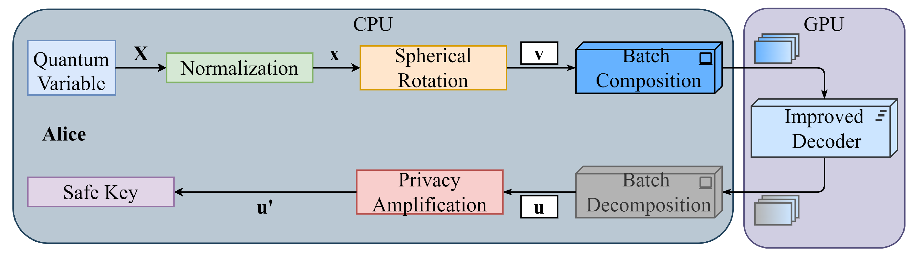
3.4. Proposed High-Speed Reconciliation Scheme

Compared with CPUs, GPUs support large-scale parallel operations, rich in computing and storage resources, and are good at floating-point operations with high precision. The most important thing is that it fits well with the proposed decoding implementation method. Therefore, we propose a high-speed reconciliation scheme based on the CPU-GPU hybrid platform. Figure 7 shows the architecture of the high-speed reconciliation scheme. We copy the data that needs to be decoded to the GPU after the reconciliation step, use the decoding network for high-speed decoding, and finally copy the decoded codewords back to the CPU for subsequent operations. The whole process makes full use of the high-speed parallel processing capability of the GPU, and we can obtain multiple secure keys in one processing.

4. Simulation Results and Performance Analysis

In this section, we will present all the experiment results in the paper. First, we provided the network training strategy. Subsequently, we carried out the performance analysis of the proposed method, including the complexity analysis of the reconciliation scheme and comparing error correction performance. Finally, we analyzed the secret key rate of the improved reconciliation scheme.

4.1. Network Training Strategy

Figure 8 shows the specific process of data set generation. Since the information bits are composed of 0 and 1, an $(\mathrm{N}-\mathrm{K},\mathrm{N})$ check matrix can generate $2^{\wedge }\mathrm{K}$ kinds of information $\mathrm{Us}$. We can obtain $2^{\wedge }\mathrm{K}$ kinds of codewords $\mathrm{Xs}$ after LDPC encoding. In the same way, we can also obtain $2^{\wedge }\mathrm{K}$ kinds of modulation information $\mathrm{Ps}$. Although the CV-QKD system works in the extremely low SNR environment, we generally use channels with different SNRs to generate sample data because the diversity of training samples is conducive to improving the model’s versatility. Theoretically, we can obtain several sets of different sample inputs $\mathrm{Vs}$ and the corresponding sample labels $\mathrm{Xs}$ through the above steps. Finally, we randomly selected samples from different SNRs to form a batch of samples.

In terms of other settings for network training, we use the Gaussian distribution method to initialize the network parameters. Moreover, we use the batch method and Adam optimizer for network training.

Table 2. The network training settings.

Items	Settings
Batch Size	200
Network Learning Rate	0.001
Network Parameter Initialization Method	Gaussian distribution method
Optimizer	Adam optimizer

illustrates the network training settings.

4.2. Complexity Analysis of Reconciliation Scheme

As we said before, the reconciliation complexity mainly focuses on the error correction process, so we mainly analyze the decoding implementation complexity. Decoding implementation complexity mainly includes the theoretical complexity and the additional specific implementation complexity. The former is mainly the mathematical operation complexity of the decoding algorithm. The latter mainly includes control operations, storage space usage, loop operations, and function calling. We denoted that $O_M$ represents the mathematical calculation complexity, $O_C$ represents the control operations complexity, $O_S$ represents the storage space usage complexity, $O_L$ represents the loop operations complexity, and $O_F$ represents the function calling complexity. Same as the definition above, a check matrix of $(M,N)$ contains E non-zero elements. Therefore, the total complexity of decoding K frame data according to the traditional LLR-BP algorithm is as follows

$$O_{\mathrm{total}}=K\ast \left(O_M+O_C+O_S+O_L+O_F\right).$$

(17)

Since $O_C$, $O_S$, and $O_L$ are all related to the matrix operation structure, we can set

$$\begin{array}{c}{O}_C=W_C\ast M\ast N,\hfill \\ O_S=W_S\ast M\ast N,\hfill \\ O_L=W_L\ast M\ast N.\hfill \end{array}$$

(18)

where $W_C$, $W_S$, and $W_L$ are weighting factors. Therefore, Equation (17) becomes

$$O_{\mathrm{total}}=K\ast \left[O_M+\left(W_C+W_S+W_L\right)\ast M\ast N+O_F\right].$$

(19)

Next, we use the proposed decoding network structure for decoding. We convert the two-dimensional matrix into a one-dimensional column vector, so we only need to pass the calculated value of the non-zero element and the weight of the corresponding layer in each iterative calculation. Therefore, the data processing amount reduces from $M\ast N$ to E (due to the sparsity of the check matrix H, $E<<M\ast N$), and the network does not require loop operations. Therefore, the total complexity becomes

$$O_{\mathrm{total}}^{\prime }=K\ast \left[O_M+\left(W_C+W_S\right)\ast E+W_L\ast 0+O_F\right].$$

(20)

In addition, the network structure is fully parallel, which means the data at the same position of each frame perform the same operation. Therefore, we can arrange the K frame data in columns to form the input matrix. According to the above ideas, each row of data in the input matrix will perform the same operation. It can be seen that we have extended the previous operation on a single data to the operation on a row of data in a matrix. This method can significantly simplify the complexity of function calling and control operations. Equation (20) may be rewritten as

$$O_{\mathrm{total}}^{″}=K\ast O_M+W_C\ast E+K\ast W_S\ast E+O_F.$$

(21)

Comparing the complexities of Equations (19) and (21), we find that using a fully parallel network structure significantly reduces the decoding implementation complexity.

In addition, the complexity of several decoding algorithms based on the same network structure is different. The most obvious difference is the computational complexity of the three algorithms. According to the above equations, we can easily find that each iteration of LLR-BP includes $2E$ additions, $(E-M)$ multiplications, E divisions, E tanh, and E arctanh operations. The linear fitting method transforms exponential operations into multiplication and addition operations. The computational complexity includes $2n$ multiplications, $(2n-1)$ additions. To balance fitting accuracy and complexity, we finally choose $n=3$. The error is small enough and will not affect the final decoding performance. Similarly, the DNNAD adds some multiplication calculations based on the LLR-BP algorithm. Therefore, the computational complexity of the three algorithms is defined as

$$\begin{array}{cc}\hfill & O_M^{\mathrm{LLR}-\mathrm{BP}}=2E_{\mathrm{add}}+{(2E-M)}_{\mathrm{mcl}}+E_{\tanh }+E_{\tanh {}^{-1}}\hfill \\ \hfill & O_M^{\mathrm{FIT}}={(2E+5)}_{\mathrm{add}}+{(4E-M+6)}_{\mathrm{mcl}}+E_{\tanh {}^{-1}}\hfill \\ \hfill & O_M^{\mathrm{DNNAD}}=2E_{\mathrm{add}}+{(3E-M)}_{\mathrm{mcl}}+E_{\tanh }+E_{\tanh {}^{-1}}\hfill \end{array}.$$

(22)

However, for the DNNAD, we should also note that the weight parameters need to occupy storage space. So, its total complexity becomes

$$O_{\mathrm{total}}^{\mathrm{DNNAD}}=K\ast O_M^{\mathrm{DNNAD}}+W_C\ast E+(K+1)\ast W_S\ast E+O_F.$$

(23)

Comparing the complexity of these three algorithms, we find that the linear fitting algorithm is the least complex and, at the same time, the DNNAD is the most complex. Nonetheless, their complexity is much lower than that of traditional decoding implementations.

Figure 9 shows the decoding speed of different decoding implementation methods on an Intel(R) Core(TM) i7-6700K CPU and an NVIDIA GeForce GTX 1650 GPU. As we analyzed, the network structure greatly improves the decoding speed. The same is true for reconciliation. Therefore, we can realize high-speed reconciliation.

4.3. Error Correction Performance Comparison

The decoding success rate is a crucial factor that affects the reconciliation performance. If the error correction fails, the entire data frame will be discarded. Therefore, we usually use the frame error rate (FER) to measure the decoding success rate, expressed as the ratio of consistent frames obtained by both terminals to the total number of frames. FER will not affect whether the system can obtain a secure key, but to improve the practicability of the system and enhance the reliability of communication, we should minimize FER.

We first constructed four check matrices with different code lengths and code rates. Then, we compared the frame error rates of different algorithms. Figure 10 shows the frame error rate of the four codewords at different iterations. We can find that the performance of linear fitting is close to that of LLR-BP and sometimes even better than LLR-BP. In addition, the DNNAD generally outperforms LLR-BP. This result confirms that the improvement ideas we analyzed before are feasible. More importantly, it proves that the proposed decoding network structure can be applied to various codewords and has strong versatility.

4.4. Secret Key Rate

As mentioned earlier, the reconciliation efficiency directly affects the secure transmission distance and secret key rate of the system. For the CV-QKD system of reverse multi-dimensional reconciliation, the secret key rate could be defined as

$$K=(1-FER)\left(\beta I_{\mathrm{AB}}-{\chi }_{\mathrm{BE}}\right).$$

(24)

where $\beta$ is the reconciliation efficiency, $I_{\mathrm{AB}}$ is the Shannon mutual information between Alice and Bob, and ${\chi }_{\mathrm{BE}}$ is the von Neumann Entropy between Bob and Eve [49,50,51]. The reconciliation efficiency is determined by the performance of the LDPC code, which can be defined as $\beta =R/C,$ where R is the code rate of the LDPC code, C is the channel capacity, and $C=1/2\ast {log}_2(1+SNR)$. When the check matrix used in reconciliation is determined, C has also been determined, and $\beta$ is the same. Both $I_{\mathrm{AB}}$ and ${\chi }_{\mathrm{BE}}$ are related to the system parameters and the transmission distance. Generally speaking, the longer the transmission distance, the lower the secret key rate. Therefore, we can increase the secret key rate by decreasing the FER.

We choose the $(98304,131072)$ check matrix for reconciliation. According to the simulation in the previous part, we can conclude that the Shannon limit is 0.45. Using the above formula, we gain that the reconciliation efficiency is $93.27\%$. Additionally, we can leverage the DNNAD to reduce FER and thus increase the secret key rate.

5. Conclusions

In this paper, we proposed a high-speed reconciliation scheme based on the CPU-GPU hybrid platform. We first proposed a decoding network structure that supports high-speed error correction considering the high complexity of reverse reconciliation based on the LDPC code. Subsequently, we used this structure to implement two improved decoding algorithms, reducing algorithm complexity or improving decoding performance. Finally, we applied the improved decoder to the system to achieve high-speed reconciliation. Since the GPU cannot reflect the advantages of the simplified algorithm, our next task is to use FPGA to realize the special chip of high-speed reconciliation.

References

1. Mafu, M. A Simple Security Proof for Entanglement-Based Quantum Key Distribution. JQIS 2016, 6, 296–303. [Google Scholar] [CrossRef] [Green Version]
2. Milicevic, M.; Feng, C.; Zhang, L.M.; Gulak, P.G. Quasi-Cyclic Multi-Edge LDPC Codes for Long-Distance Quantum Cryptography. Npj Quantum Inf. 2018, 4, 21. [Google Scholar] [CrossRef] [Green Version]
3. Bennett, C.H.; Brassard, G. Quantum Cryptography: Public Key Distribution and Coin Tossing. Theor. Comput. Sci. 2014, 560, 7–11. [Google Scholar] [CrossRef]
4. Bennett, C.H. Quantum Cryptography Using Any Two Nonorthogonal States. Phys. Rev. Lett. 1992, 68, 3121–3124. [Google Scholar] [CrossRef]
5. Grosshans, F.; Grangier, P. Continuous Variable Quantum Cryptography Using Coherent States. Phys. Rev. Lett. 2002, 88, 057902. [Google Scholar] [CrossRef] [Green Version]
6. Lodewyck, J.; Bloch, M.; García-Patrón, R.; Fossier, S.; Karpov, E.; Diamanti, E.; Debuisschert, T.; Cerf, N.J.; Tualle-Brouri, R.; McLaughlin, S.W.; et al. Quantum Key Distribution over 25 km with an All-Fiber Continuous-Variable System. Phys. Rev. A 2007, 76, 042305. [Google Scholar] [CrossRef] [Green Version]
7. Cao, Y.; Zhao, Y.; Wang, Q.; Zhang, J.; Ng, S.X.; Hanzo, L. The Evolution of Quantum Key Distribution Networks: On the Road to the Qinternet. IEEE Commun. Surv. Tutor. 2022. [Google Scholar] [CrossRef]
8. Pirandola, S.; Andersen, U.L.; Banchi, L.; Berta, M.; Bunandar, D.; Colbeck, R.; Englund, D.; Gehring, T.; Lupo, C.; Ottaviani, C.; et al. Advances in Quantum Cryptography. Adv. Opt. Photon. 2020, 12, 1012. [Google Scholar] [CrossRef] [Green Version]
9. Jouguet, P.; Kunz-Jacques, S.; Leverrier, A. Long-Distance Continuous-Variable Quantum Key Distribution with a Gaussian Modulation. Phys. Rev. A 2011, 84, 062317. [Google Scholar] [CrossRef] [Green Version]
10. VanAssche, G.; Cardinal, J.; Cerf, N.J. Reconciliation of a Quantum-Distributed Gaussian Key. IEEE Trans. Inform. Theory 2004, 50, 394–400. [Google Scholar] [CrossRef] [Green Version]
11. Grosshans, F.; Cerf, N.J.; Wenger, J.; Tualle-Brouri, R.; Grangier, P. Virtual Entanglement and Reconciliation Protocols for Quantum Cryptography with Continuous Variables. arXiv 2003, arXiv:quant-ph/0306141. [Google Scholar] [CrossRef]
12. Fang, J.; Huang, P.; Zeng, G. Multichannel Parallel Continuous-Variable Quantum Key Distribution with Gaussian Modulation. Phys. Rev. A 2014, 89, 022315. [Google Scholar] [CrossRef] [Green Version]
13. Gallager, R. Low-Density Parity-Check Codes. IEEE Trans. Inform. Theory 1962, 8, 21–28. [Google Scholar] [CrossRef] [Green Version]
14. Xie, J.; Wu, H.; Xia, C.; Ding, P.; Song, H.; Xu, L.; Chen, X. High Throughput Error Correction in Information Reconciliation for Semiconductor Superlattice Secure Key Distribution. Sci. Rep. 2021, 11, 3909. [Google Scholar] [CrossRef]
15. Wang, C.; Huang, D.; Huang, P.; Lin, D.; Peng, J.; Zeng, G. 25 MHz Clock Continuous-Variable Quantum Key Distribution System over 50 Km Fiber Channel. Sci. Rep. 2015, 5, 14607. [Google Scholar] [CrossRef] [Green Version]
16. Wang, X.; Zhang, Y.; Yu, S.; Guo, H. High Speed Error Correction for Continuous-Variable Quantum Key Distribution with Multi-Edge Type LDPC Code. Sci. Rep. 2018, 8, 10543. [Google Scholar] [CrossRef] [Green Version]
17. Mao, H.; Li, Q.; Han, Q.; Guo, H. High-Throughput and Low-Cost LDPC Reconciliation for Quantum Key Distribution. Quantum Inf. Process 2019, 18, 232. [Google Scholar] [CrossRef] [Green Version]
18. Li, Y.; Zhang, X.; Li, Y.; Xu, B.; Ma, L.; Yang, J.; Huang, W. High-Throughput GPU Layered Decoder of Quasi-Cyclic Multi-Edge Type Low Density Parity Check Codes in Continuous-Variable Quantum Key Distribution Systems. Sci. Rep. 2020, 10, 14561. [Google Scholar] [CrossRef]
19. Zhang, K.; Huang, X.; Wang, Z. High-Throughput Layered Decoder Implementation for Quasi-Cyclic LDPC Codes. IEEE J. Select. Areas Commun. 2009, 27, 985–994. [Google Scholar] [CrossRef]
20. Lin, D.; Huang, D.; Huang, P.; Peng, J.; Zeng, G. High Performance Reconciliation for Continuous-Variable Quantum Key Distribution with LDPC Code. Int. J. Quantum Inform. 2015, 13, 1550010. [Google Scholar] [CrossRef]
21. Daesun, O.; Parhi, K.K. Min-Sum Decoder Architectures With Reduced Word Length for LDPC Codes. IEEE Trans. Circuits Syst. I 2010, 57, 105–115. [Google Scholar] [CrossRef]
22. Hinton, G.E.; Osindero, S.; Teh, Y.-W. A Fast Learning Algorithm for Deep Belief Nets. Neural Comput. 2006, 18, 1527–1554. [Google Scholar] [CrossRef]
23. Nachmani, E.; Be’ery, Y.; Burshtein, D. Learning to Decode Linear Codes Using Deep Learning. In Proceedings of the 2016 54th Annual Allerton Conference on Communication, Control, and Computing (Allerton), Monticello, IL, USA, 27–30 September 2016; pp. 341–346. [Google Scholar]
24. Liang, F.; Shen, C.; Wu, F. An Iterative BP-CNN Architecture for Channel Decoding. IEEE J. Sel. Top. Signal Process. 2018, 12, 144–159. [Google Scholar] [CrossRef] [Green Version]
25. Lugosch, L.; Gross, W.J. Neural Offset Min-Sum Decoding. In Proceedings of the 2017 IEEE International Symposium on Information Theory (ISIT), Aachen, Germany, 25–30 June 2017; pp. 1361–1365. [Google Scholar]
26. Zeng, G. Quantum Private Communication; Springer: Berlin/Heidelberg, Germany, 2010; ISBN 978-3-642-03295-0. [Google Scholar]
27. Bennett, C.H.; Brassard, G.; Crepeau, C.; Maurer, U.M. Generalized Privacy Amplification. IEEE Trans. Inform. Theory 1995, 41, 1915–1923. [Google Scholar] [CrossRef] [Green Version]
28. Deutsch, D.; Ekert, A.; Jozsa, R.; Macchiavello, C.; Popescu, S.; Sanpera, A. Quantum Privacy Amplification and the Security of Quantum Cryptography over Noisy Channels. Phys. Rev. Lett. 1996, 77, 2818–2821. [Google Scholar] [CrossRef] [Green Version]
29. Bennett, C.H.; Brassard, G.; Robert, J.-M. Privacy Amplification by Public Discussion. SIAM J. Comput. 1988, 17, 210–229. [Google Scholar] [CrossRef]
30. Silberhorn, C.; Ralph, T.C.; Lütkenhaus, N.; Leuchs, G. Continuous Variable Quantum Cryptography: Beating the 3 DB Loss Limit. Phys. Rev. Lett. 2002, 89, 167901. [Google Scholar] [CrossRef] [Green Version]
31. Leverrier, A.; Alléaume, R.; Boutros, J.; Zémor, G.; Grangier, P. Multidimensional Reconciliation for a Continuous-Variable Quantum Key Distribution. Phys. Rev. A 2008, 77, 042325. [Google Scholar] [CrossRef] [Green Version]
32. Leverrier, A.; Grangier, P. Continuous-Variable Quantum Key Distribution Protocols with a Discrete Modulation. arXiv 2011, arXiv:1002.4083. [Google Scholar]
33. Chen, J.; Fossorier, P.M.C. Density Evolution for BP-Based Decoding Algorithms of LDPC Codes and Their Quantized Versions. In Proceedings of the Global Telecommunications Conference, 2002. GLOBECOM ’02, Taipei, Taiwan, 17–21 November 2002; Volume 2, pp. 1378–1382. [Google Scholar]
34. Richardson, T.J.; Urbanke, R.L. The Capacity of Low-Density Parity-Check Codes under Message-Passing Decoding. IEEE Trans. Inform. Theory 2001, 47, 599–618. [Google Scholar] [CrossRef]
35. Wei, X.; Akansu, A.N. Density Evolution for Low-Density Parity-Check Codes under Max-Log-MAP Decoding. Electron. Lett. 2001, 37, 1125. [Google Scholar] [CrossRef]
36. Anastasopoulos, A. A Comparison between the Sum-Product and the Min-Sum Iterative Detection Algorithms Based on Density Evolution. In Proceedings of the GLOBECOM’01. IEEE Global Telecommunications Conference (Cat. No.01CH37270), San Antonio, TX, USA, 25–29 November 2001; Volume 2, pp. 1021–1025. [Google Scholar]
37. Tanner, R. A Recursive Approach to Low Complexity Codes. IEEE Trans. Inform. Theory 1981, 27, 533–547. [Google Scholar] [CrossRef] [Green Version]
38. Luby, M.G.; Mitzenmacher, M.; Shokrollahi, M.A.; Spielman, D.A. Improved Low-Density Parity-Check Codes Using Irregular Graphs. IEEE Trans. Inform. Theory 2001, 47, 585–598. [Google Scholar] [CrossRef] [Green Version]
39. Chen, J.; Fossorier, M.P.C. Near Optimum Universal Belief Propagation Based Decoding of Low-Density Parity Check Codes. IEEE Trans. Commun. 2002, 50, 406–414. [Google Scholar] [CrossRef]
40. Forney, G.D. Codes on Graphs: Normal Realizations. IEEE Trans. Inform. Theory 2001, 47, 520–548. [Google Scholar] [CrossRef] [Green Version]
41. Etzion, T.; Trachtenberg, A.; Vardy, A. Which Codes Have Cycle-Free Tanner Graphs? IEEE Trans. Inform. Theory 1999, 45, 2173–2181. [Google Scholar] [CrossRef] [Green Version]
42. Yang, N.; Jing, S.; Yu, A.; Liang, X.; Zhang, Z.; You, X.; Zhang, C. Reconfigurable Decoder for LDPC and Polar Codes. In Proceedings of the 2018 IEEE International Symposium on Circuits and Systems (ISCAS), Florence, Italy, 27–30 May 2018; pp. 1–5. [Google Scholar]
43. Huang, D.; Huang, P.; Wang, T.; Li, H.; Zhou, Y.; Zeng, G. Continuous-Variable Quantum Key Distribution Based on a Plug-and-Play Dual-Phase-Modulated Coherent-States Protocol. Phys. Rev. A 2016, 94, 032305. [Google Scholar] [CrossRef]
44. Gardner, M.W.; Dorling, S.R. Artificial Neural Networks (the Multilayer Perceptron)—A Review of Applications in the Atmospheric Sciences. Atmos. Environ. 1998, 32, 2627–2636. [Google Scholar] [CrossRef]
45. Gruber, T.; Cammerer, S.; Hoydis, J.; Brink, S. On Deep Learning-Based Channel Decoding. In Proceedings of the 2017 51st Annual Conference on Information Sciences and Systems (CISS), Baltimore, MD, USA, 22–24 March 2017; pp. 1–6. [Google Scholar]
46. Caruana, R. Multitask Learning. Mach. Learn. 1997, 28, 41–75. [Google Scholar] [CrossRef]
47. Albawi, S.; Mohammed, T.A.; Al-Zawi, S. Understanding of a Convolutional Neural Network. In Proceedings of the 2017 International Conference on Engineering and Technology (ICET), Antalya, Turkey, 21–23 August 2017; pp. 1–6. [Google Scholar]
48. Kim, J.-K.; Lee, M.-Y.; Kim, J.-Y.; Kim, B.-J.; Lee, J.-H. An Efficient Pruning and Weight Sharing Method for Neural Network. In Proceedings of the 2016 IEEE International Conference on Consumer Electronics-Asia (ICCE-Asia), Seoul, Korea, 26–28 October 2016; pp. 1–2. [Google Scholar]
49. Huang, D.; Huang, P.; Lin, D.; Zeng, G. Long-Distance Continuous-Variable Quantum Key Distribution by Controlling Excess Noise. Sci. Rep. 2016, 6, 19201. [Google Scholar] [CrossRef] [Green Version]
50. Fossier, S.; Diamanti, E.; Debuisschert, T.; Villing, A.; Tualle-Brouri, R.; Grangier, P. Field Test of a Continuous-Variable Quantum Key Distribution Prototype. New J. Phys. 2009, 11, 045023. [Google Scholar] [CrossRef]
51. Guo, Y.; Liao, Q.; Wang, Y.; Huang, D.; Huang, P.; Zeng, G. Performance Improvement of Continuous-Variable Quantum Key Distribution with an Entangled Source in the Middle via Photon Subtraction. Phys. Rev. A 2017, 95, 032304. [Google Scholar] [CrossRef] [Green Version]
Figure 1. Flow chart of post-processing of reverse multi-dimensional reconciliation. Since decoding is the crucial step in reconciliation, we can improve the reconciliation performance by improving the decoding performance.
Photonics 09 00110 g001
Figure 2. (a) The structure of the Tanner graph corresponds to Equation (2). (b) Node information transmitted in the Tanner graph. L ( r j i ) is the check node update information transmitted from the check node C j to the variable node V i . L ( q i j ) is the variable node update information transmitted from the variable node V i to the check node C j .
Photonics 09 00110 g002
Figure 3. The structure diagram of a single hidden layer MLP. The depth of the network is 3, and the number of neurons in the input layer, hidden layer, and output layer is 3, 6, and 3, respectively.
Photonics 09 00110 g003
Figure 4. The proposed decoding network structure. The entire network consists of one input layer, ( 2 I 1 ) hidden layers, and one output layer, where I is the maximum number of iterations. The input and output layers contain N neurons, corresponding to Equations (3) and (6). Iterations except the last iteration correspond to two hidden layers with E neurons, named c2v_layer and v2c_layer, respectively corresponding to Equations (4) and (5), where E is the number of non-zero elements of the check matrix.
Photonics 09 00110 g004
Figure 5. The network structure of (9) with 3 hidden layers corresponds to 2 iterations.
Photonics 09 00110 g005
Figure 6. The proposed deep neural network-assisted decoder (DNNAD). (a) The general model of the simulation system based on the DNNAD. (b) The network structure of the DNNAD. The structure has not changed in the application phase, but some weights are added to the forward propagation. In the training phase, we add some additional branches to output the decoded codewords of each iteration based on the original network structure, so the number of hidden layers becomes ( 3 I 2 ) , where I is the maximum number of iterations.
Photonics 09 00110 g006
Figure 7. The architecture of the high-speed reconciliation scheme based on the CPU-GPU hybrid platform.
Photonics 09 00110 g007
Figure 8. Specific process of data set generation.
Photonics 09 00110 g008
Figure 9. The decoding speed of different decoding implementation methods. The speed of serial network decoding reaches 0.339 Mbits/s, which is already better than the original BP algorithm. The speed of parallel network decoding even reaches 26.7 Mbits/s on an NVIDIA GeForce GTX 1650 GPU.
Photonics 09 00110 g009
Figure 10. (a) The FER performance of ( 144 , 576 ) at 25 and 100 iterations. (b) The FER performance of ( 1408 , 1920 ) at 25 and 100 iterations. (c) The FER performance of ( 7040 , 9600 ) at 25 and 100 iterations. (d) The FER performance of ( 98304 , 131072 ) at 25 and 100 iterations.
Photonics 09 00110 g010