Article

Effect of Lidar Receiver Field of View on UAV Detection

1
Institute of Applied Electronics, China Academy of Engineering Physics, Mianyang 621900, China
2
Graduate School, China Academy of Engineering Physics, Beijing 100088, China
3
State Key Laboratory of Pulsed Power Laser Technology, Changsha 410073, China
*
Author to whom correspondence should be addressed.
Photonics 2022, 9(12), 972; https://doi.org/10.3390/photonics9120972
Submission received: 4 November 2022 / Revised: 30 November 2022 / Accepted: 2 December 2022 / Published: 11 December 2022

Abstract

:
Researchers have shown that single-photon light detection and ranging (lidar) is highly sensitive and has a high temporal resolution. Due to the excellent beam directivity of lidar, most applications focus on ranging and imaging. Here, we present a lidar detection system for night environments. Different from MEMS, we choose a large divergence rather than scanning to detect unmanned aerial vehicles (UAVs). Collection and detection are achieved through the use of high-efficiency optical devices. With time-correlated single photon counting (TCSPC), we performed subsequent drone search work at centimeter resolution. We believe that we have developed a new technique for detecting UAVs. We show how the field of view influences the detection process. For some key areas of air defense, it is extremely necessary to find UAVs quickly and in a timely manner. In short, the results represent an important step toward practical, low-power drone detection using lidar.

1. Introduction

UAVs have become increasingly popular in recent years. The worldwide availability of low-cost unmanned aerial vehicles (UAVs) that are easy to operate has led to increasing problems. These problems range from misuse of toys to the abusive use of UAVs for spying or other hostile activities. Consequently, lidar for drone detection in Earth’s atmosphere has received increased research attention, especially with regard to sensitive areas such as airports, company premises or military facilities [1]. Because of the small size of UAVs and their small radar section, drones are difficult to detect at long distances by lidars [2]. During long-range detection, the Earth’s atmosphere will decrease the number of echoed photons as the distance increases [3]. Most of the previously published studies have focused on using light spots to scan UAV-like targets for detection through methods that increase the scanning spot density, these methods include the micro-electro-mechanical system (MEMS), in which galvanometers are used to obtain a large field of view (FOV) [4]. In order to achieve effective scanning and detection of the airspace by a laser beam, the commonly used LIDAR scanning methods include raster scanning, Lissajous scanning, spiral scanning, etc. [5,6,7]. MEMS is a detection method that obtains a large field of view by fast scanning, which is essentially a small FOV ranging work. Nonetheless, there is still some time disadvantage during successive scans [8].
TCSPC-based single-photon lidar [9] is capable of achieving single-photon sensitivity and picosecond resolution for time-of-flight measurements [10]. Experimental developments in various applications have made significant progress and are expected to continue, including for autonomous rendezvous docking in space, space target detection, navigation for unmanned aerial vehicles (UAVs), advanced driver assistance systems (ADAS), automatic driving, and so on [11]. USTC’s lab has successfully implemented single-photon imaging experiments on targets 200 km away [12]. Over 90 satellites are being tracked by the laser ranging stations established by the International Laser Ranging Service (ILRS) from low Earth orbit to geosynchronous orbit and retroreflector arrays on the surface of the Moon [13].
The first investigator who considered the application of scanning light detection and ranging (LiDAR) systems is Church [14]. Using a scanning LiDAR system which scans in circular patterns, they discussed the probability for the detection of a UAV when it is in the field of view (FOV) of the sensor. In a US patent [15] a two-component scanning LIDAR system is described for 360-degree environmental surveillance that includes a LiDAR system with a narrow FOV for UAV identification.
With the aim of overcoming the shortcoming of the small FOV, a high-efficiency, high single-to-noise ratio (SNR) heteraxial single-photon lidar system with a giant laser spot for UAV detection is proposed in this article. This system consists of variable focus optical lenses, a low-noise single-photon avalanche diode detector (SPAD), and a TCSPC system. Furthermore, we concentrate on how the FOV affects the detection accuracy.
In this paper, we try to use lidar to detect drones. The review is structured as follows: in Section 2, a single-photon lidar system model is proposed. Then the principles of the lidar are presented. Section 3 summarizes the search principles of the entire search radar, as well as the sources of atmospheric loss and noise, and uses the Monte Carlo method to simulate the UAV search experiment and the conducted UAV search experiments under different field of view angles. The lidar experiment validates our modeling and demonstrates accurate depth estimation with different FOV. Section 3.2 explains the experimental results and sources of error. The discussion and conclusions are discussed in Section 4 and Section 5, respectively.

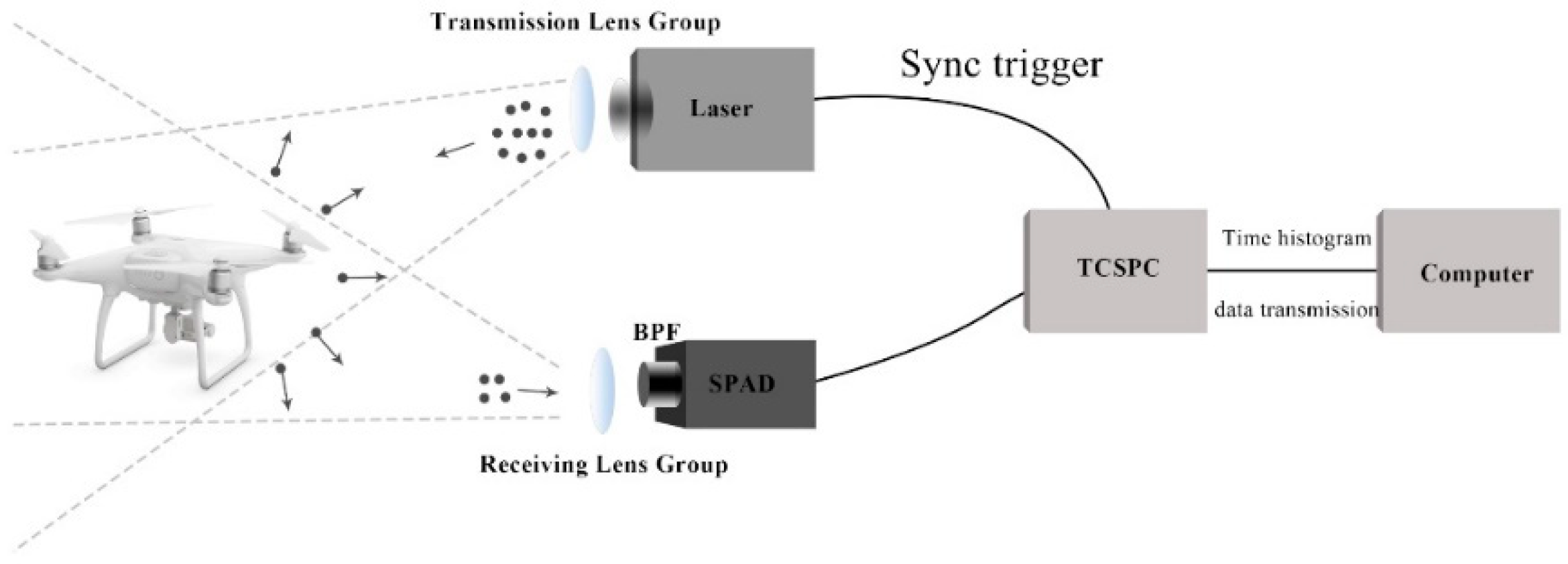
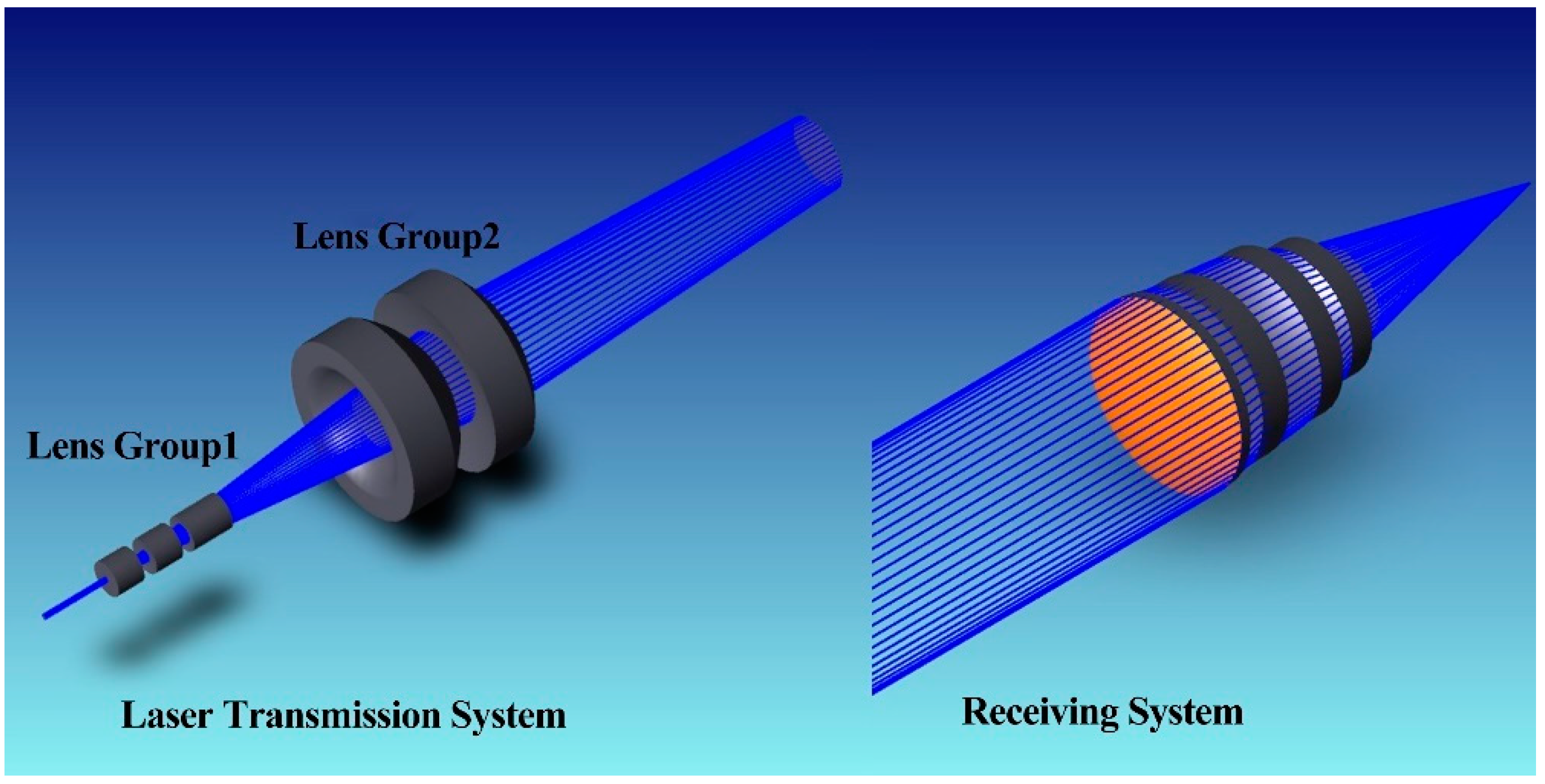
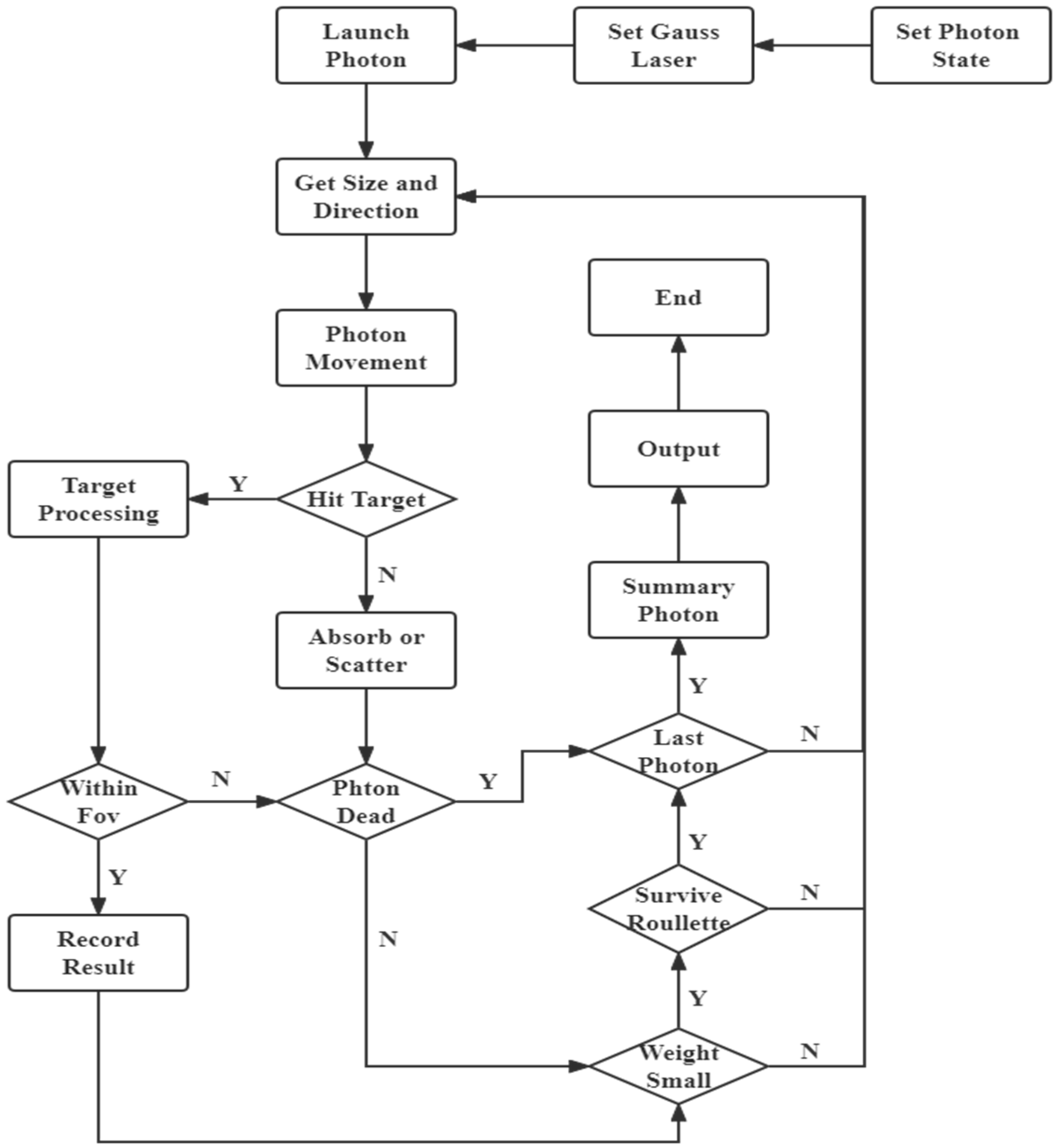
2. Single-Photon Lidar Process

As shown in Figure 1, this heteraxial lidar system is typically based on commercially available devices that run at normal atmospheric temperature, where the laser source is a diode-pumped solid-state laser (Onda 1064 nm, bright SOLUTION, Pavia, Italy) working at 1064 nm and a compact and in which a low-noise Si-SPAD detector is used. Several advantages of using a near-infrared wavelength include reduced solar background and low atmospheric absorption loss [16]. The maximal pulse energy transmitted was 37 μJ. In order to transmit the laser, a commercial Galileo telescope with variable focal length and a modest aperture of 50 mm was coupled with a custom optical table that can be rotated. We can change the divergence angle by changing the lens position. The reflected photons are collected into the Si-SPAD with an appropriate diameter core (12.6 μm) to ensure high-efficiency collection.
Using a TCSPC module, we recorded the time gaps between photon detections and the most current laser emission and sent them to a computer for analysis [17]. Since the time jitter of the TCSPC system and the single-photon detector is much smaller than the laser pulse width, the lidar time jitter of the whole system was assumed to be 10 ns in our study.
Because the number of photons reflected by UAV-like targets in long-range lidar is highly limited, the background noise in this detection system must be very low [18,19]. So, a 10-nm band-pass filter (BPF) centered on a laser of 1064 nm wavelength was placed in front of the objective to reduce the background noise. When a BPF is placed in front of the receiving system, laser pulse backscatter is responsible for most of the noise generated by near-field atmospheres and standard receiving optical devices [12]. For other parameters of the system, see Table 1. Additionally, the laser transmission system and receiving system are shown in the Figure 2. By changing the distance between the mirror group 1 and the mirror group 2, the divergence angle of the laser light can be changed.

3. Laser Searching Experiment at 1064 nm
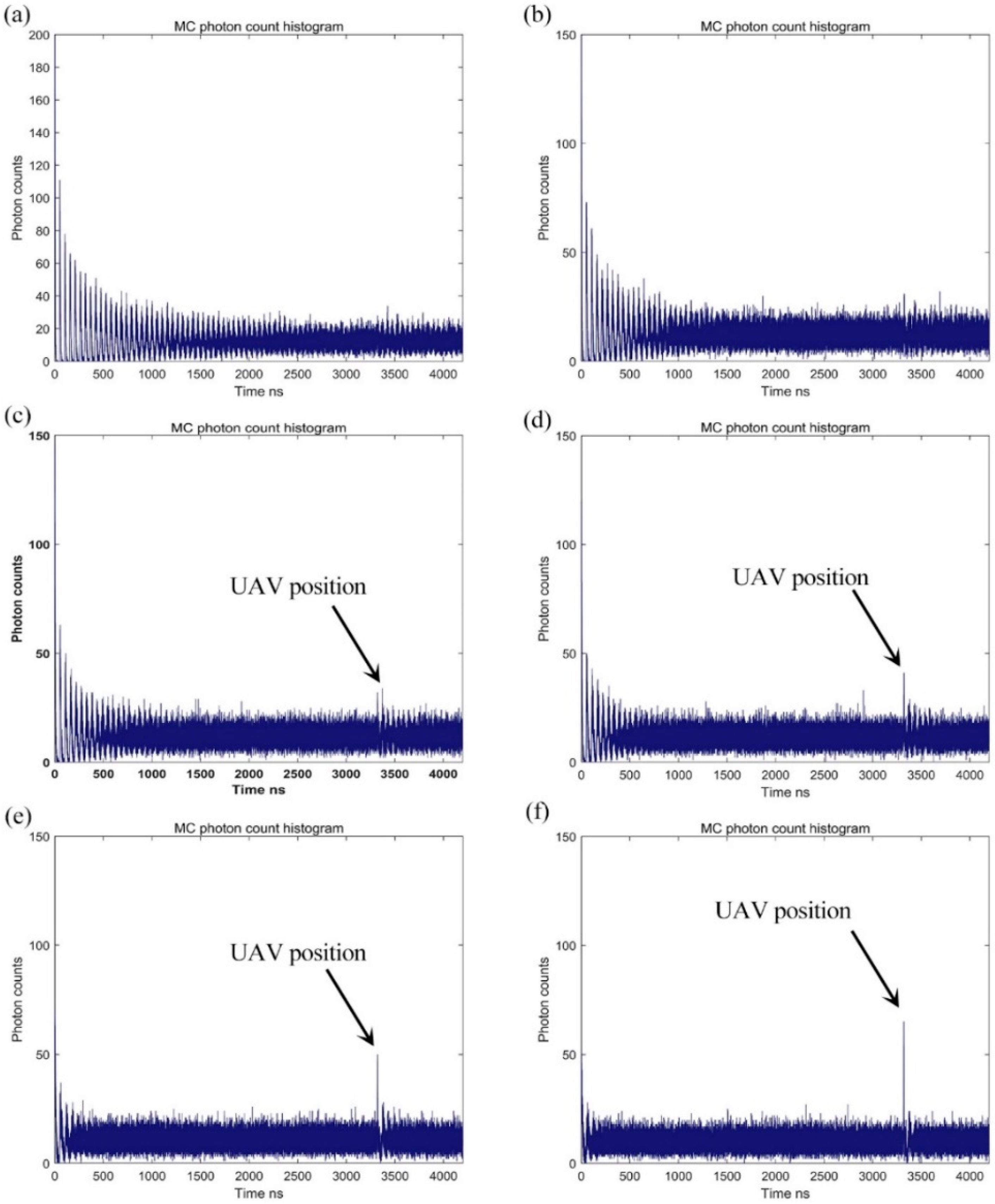
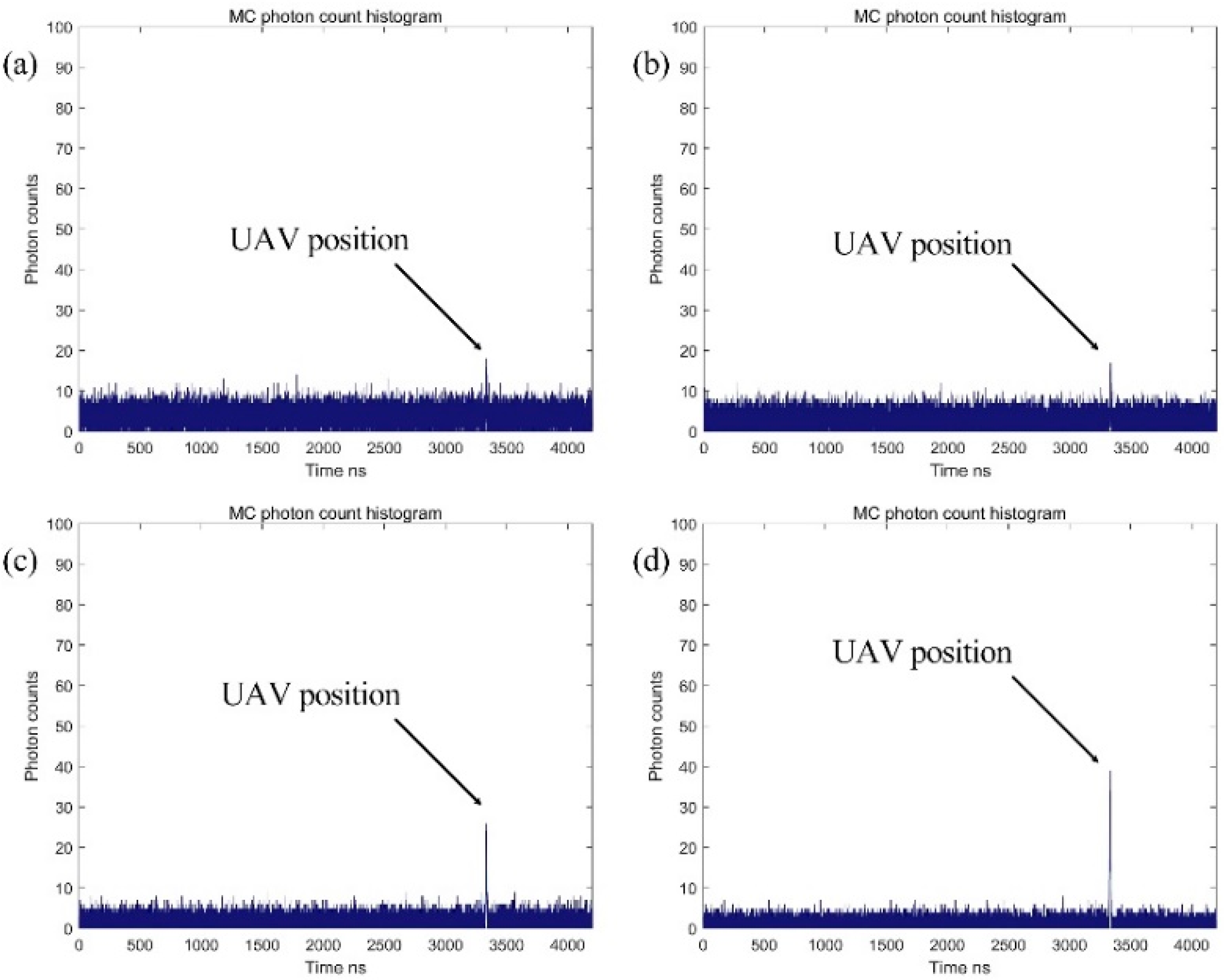
3.1. Simulation

When the laser is emitted from the laser to be thereby received by the receiving system, the transmission energy is reduced due to the interference of atmospheric molecules and aerosol molecules. Under uniform atmospheric conditions [20], the one-way transmission T ( R , λ ) in the horizontal path can be expressed by the following equation:
T ( R , λ ) = exp { [ k m ( λ ) + k a ( λ ) + r m ( λ ) + r a ( λ ) ] R } = exp [ σ T ( λ ) R ]
where k m ( λ ) is atmospheric molecular absorption coefficient, k a ( λ ) is the atmospheric aerosol absorption coefficient, r m ( λ ) is the atmospheric molecular scattering coefficient, r a ( λ ) is the scattering coefficient of atmospheric aerosol particles, R is the distance from the target to the system, and σ T ( λ ) is the atmospheric extinction coefficient. For the lower atmosphere, the atmosphere extinction coefficient σ T ( λ ) is given by [21]:
σ T ( λ ) = 3.91 D × ( 550 λ ) q
where D is the atmospheric visibility and q is the correction factor, when the atmospheric visibility is between 6 and 40 km, q = 1.3   [22,23,24].
For search lidar, the following equation expresses the power of the echo signal:
P r = ρ × T a 2 × η t × η r × c o s θ t × A t A l × A r π × R 2 × P t
here P r is the power of the laser echo, T a is a one-way transmittance of laser transmission in the atmosphere, and η t × η r represents the total efficiency of the optical system and c o s θ t . A default value is 1, which is the normal angle between the optical axis of the laser emission system and the target drone. ρ is the target scattering coefficient. The UAVs target material is relatively complex. The commonly used materials are engineering plastics and carbon fiber composite materials [25,26]. We used UAV DJI Phantom4, which can be equivalent to engineering plastic drones with ρ = 0.6 . A t A l is the ratio of the target scattering effective area to the irradiated spot area at the target position. A r is the receiving aperture area, R is the distance from the detection system to the target and P t is the peak power of the laser emission signal. Equation to convert P r to the number of photons N r given by:
N r = P r F · E p = P r · λ F · h · c
where F is the frequency of the laser, c is the speed of light.
For UAV searches working in a daylight environment, the background noise of the sky is the key to affecting the search efficiency and even determining the success of the search. The standard deviation of the background signal can be determined, for example, from samples obtained before the laser was emitted or from samples corresponding to very high altitudes where the laser’s backscatter is barely noticeable compared with the background signal [27]. The daytime sky background noise consists mainly of the reflection of sunlight, the sun’s scattering by the atmosphere, and sunlight radiation, which has a value 104~106 times greater than at night.
In the daytime, at a wavelength of 1064 nm, the thermal radiation of the target is much smaller than the scattering of sunlight, so the thermal radiation of the target can be ignored in the analysis.
Black body radiation from objects is given by:
P B b = ϵ σ T T 4 Δ λ Ω R A r π η r
Therefore, the background noise N b b ( K ) given by:
N B s = λ h c × π 16 E · ρ · T α · A r · η r · Δ λ   · cos ( 90 θ s u n ) · θ r 2
N N s = λ h c × π 16 E · I s · T α · A r · η r · Δ λ   · cos ( 90 θ s u n ) · θ r 2
N b b = N b s + N N s
where θ s u n is the solar altitude angle; E is the solar spectral irradiance, with a value of 614.4 at 1064 nm; Δ λ is the bandwidth of BPF; and θ r is the received field of view angle. Considering the dimension in which the test site is located, the maximum value θ s u n   m a x = 80.5 ° and I S is atmospheric scattering coefficient. To ensure that UAV-like targets can be detected at noon, θ s u n   m a x = 80.5 ° was considered for the simulation. When the noise rate is greater than the saturation count rate of the detector, the target will not be detected, and thus a maximum field of view will necessarily exist at the time of detection. After the single-photon sensor and the laser energy are determined, the receiving FOV becomes the key to improving the search efficiency.
In the process of simulating the laser transmission, we used the Monte Carlo method, which does not require analytical calculation of the radiation transmission equation when solving the radiation transmission problem, but transforms the entire radiation transmission process into a random sampling statistical process, i.e., when seen as a complete Markov chain, the light source beam is regarded as a photon packet composed of a large number of photons in the calculation process. The solution process of radiative transmission is thus the process of interaction between photons and atmospheric molecules, aerosols, and cloud particles and other atmospheric media. The collision process constitutes a Markov chain. The Gaussian waveform of the laser is:
F ( t ) = A e t 2 2 ( P w ) 2
Such a laser has a shaped waveform with a Gaussian function. Other types of shaped waveforms might be of great interest. Here, this waveform is a second order temporal Gaussian beam. In the formula, the Gaussian spectrum is proportional to pulse rise time which is proportional to Pw. In addition, the time–bandwidth product is derived in terms of both the spectral and temporal widths, FWHM [28]. Where P w is FWHM of the laser pulse, A is average peak photon number in time slot. Desirable waveforms are possible to generate in the field of digital communication and have been the subject of great interest in LIDAR applications, including first range-resolved detection and identification of airborne bioaerosols using nonlinear lidar [29].
The flow chart of the whole simulation is shown in Figure 3. When the Monte Carlo method solves the radiation transfer problem, it converts the entire radiation transfer process into a random sampling statistical process, which is regarded as a complete Markov chain. In the calculation process, the light source beam is regarded as being composed of a large number of photons The solution process of photon packet and radiative transfer is the process of interaction between photons and atmospheric media such as atmospheric molecules, aerosols, and cloud particles. The entire random collision process constitutes a Markov chain. The steps for using the Monte Carlo method to simulate the photon transmission process of the UAV detection process are as follows. Firstly, one must initialize the light source and receiver, where the initialization of the light source includes the energy, azimuth and number of photons of the light source, and the initialization of the receiver is primarily the initialization of the receiver position and angle, receiving area, and receiving field of view. Secondly, one must undertake the transmission process of sampling photons, including the random generation of the emission angle and position of photons, and samplings of both the type of medium interacting with photons and the photons before each collision. For the transmission distance, the state of the photon is updated by using the single scattering albedo, the new azimuth angle of the photon is determined by the random number, and the new scattering angle of the photon is calculated by using the phase function.
The initialization process includes the initialization of the optical properties of the three-dimensional atmosphere and initialization of the photon state, wherein the initialization of the three-dimensional atmosphere includes the extinction coefficient, as well as the single scattered albedo and its phase function. The scattering phase function is often used to calculate the new transmission direction after the photon collides with the scattering medium. Here we use the Henyey–Greenstein (H–G) phase function improved by Cornette and Shanks [30]
P ( θ ) = 3 2 · 1 g 2 2 + g 2 · 1 + ( c o s θ ) 2 ( 1 + g 2 2 g c o s θ ) 3 2
The Monte Carlo method mainly traces the state characteristics such as the motion position ( X , Y , Z ) , the motion direction ( μ x , μ y , μ z ) , the motion step s, the motion time t, and the weight of the photon when it is transmitted in the air, and simulates the scattering of photons and molecules and particles in the air, as well as action processes such as absorption and reflection at the target location. The new coordinates of the photon during the simulation are expressed by the following formulas
{ Z N E W = X + l μ x Y N E W = Y + l μ y Z N E W = Z + l μ z
where
{ μ x = s i n θ s i n ϕ u y = s i n θ c o s ϕ u z = c o s θ
Due to the existence of two processes of scattering and absorption in the atmosphere, in order to improve the computational efficiency in the Monte Carlo photon tracing process, an initial weight is assigned to each emitted photon and the probability of scattering is calculated, that is, the single scattering rate ω 0 will change the current weight. The calculation method is given by:
W e i g h t n e w = w e i g h t × ω 0
During the transmission process for the photons, the weight continually decreases and the influence on signal detection continually weakens. The death threshold of photons is initially set as the criterion for ending photon tracing. If the weight of the photon is lower than the threshold, Russian roulette is used to judge whether the photon can increase the weight and continue to move.
We simulated the UAV search at different field-of-view angles in night-time environment, i.e., at different background noise rates. As shown in Figure 4a–f, we simulated the target’s echoes at 500 m for different field of view angles. Figure 4a,b show the situation when the noise rate is higher than the saturation count rate of the detector. The fields of view utilized in Figure 4c–f are 0.9 mrad, 0.8 mrad, 0.6 mrad, and 0.5 mrad, respectively, to illustrate the echo at different noise rates.
Because of the presence of single-photon detector dark noise, we formulated θ s u n   m i n = 0.001 ° in the evening, with the noise rate near 2 MHz. Figure 5a–d shows the echo histogram in a dark environment where the target is 500 m away. The FOV shown in Figure 4a–d are 40 mrad, 30 mrad, 25 mrad, and 20 mrad, respectively. With the decrease of the FOV, we can clearly observe the SNR is gradually increasing.
We also noticed that the SNR of the target echo could not be identified if the target was too far away, even if the noise rate did not overcome the saturation count rate of the detector. Figure 6a–d show the detection result of the different ranges of UAV targets.
With increasing FOV, the return signal from the target was so highly attenuated that to ensure the efficiency of the searching program, it became necessary to select an FOV that allowed the algorithm to process the SNR later. By simulating a sequence of detections containing a particular parameter, we demonstrate that the Markov chain limiting distribution used in this paper approximates the distribution of detection times and is reliable.

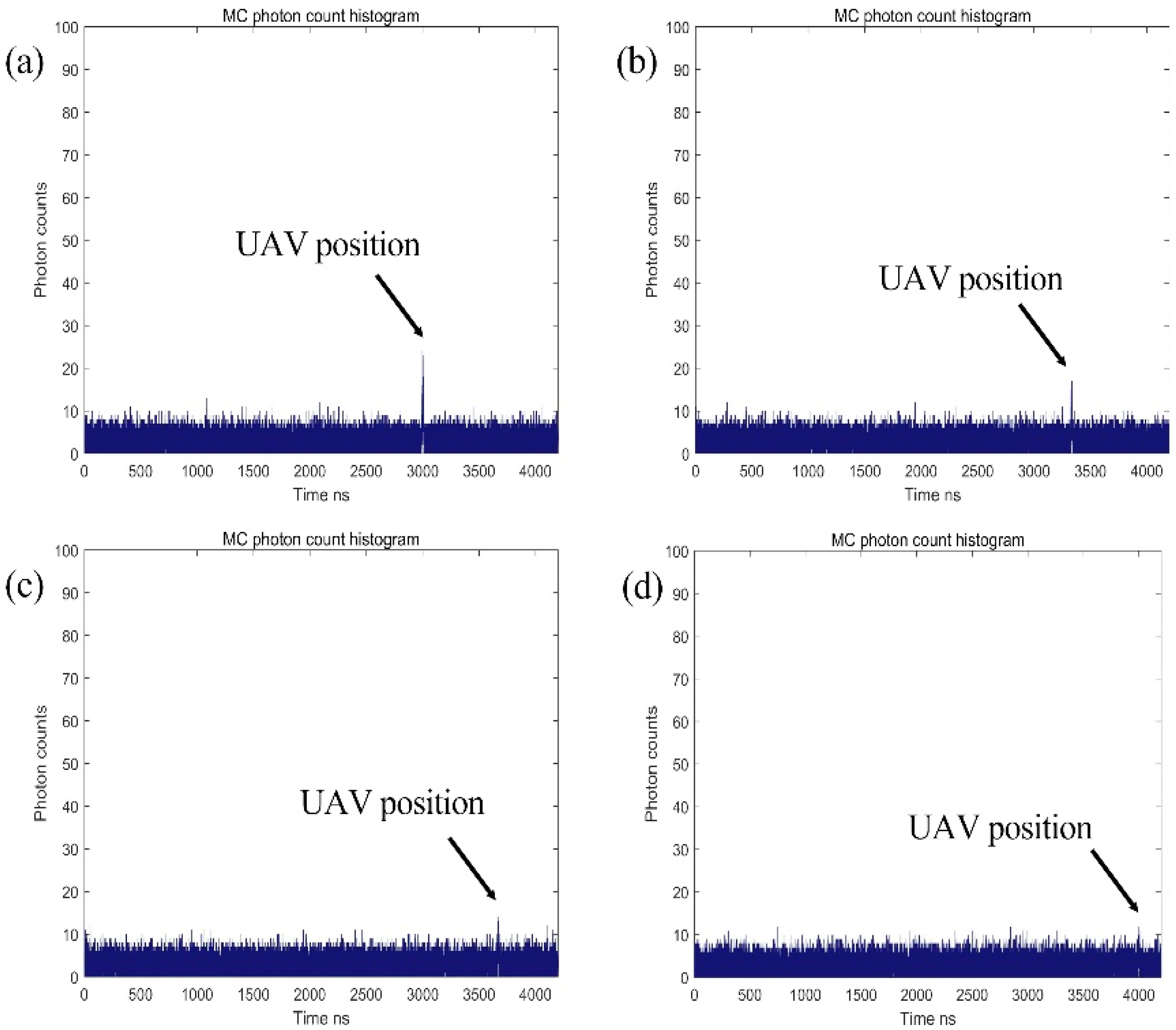
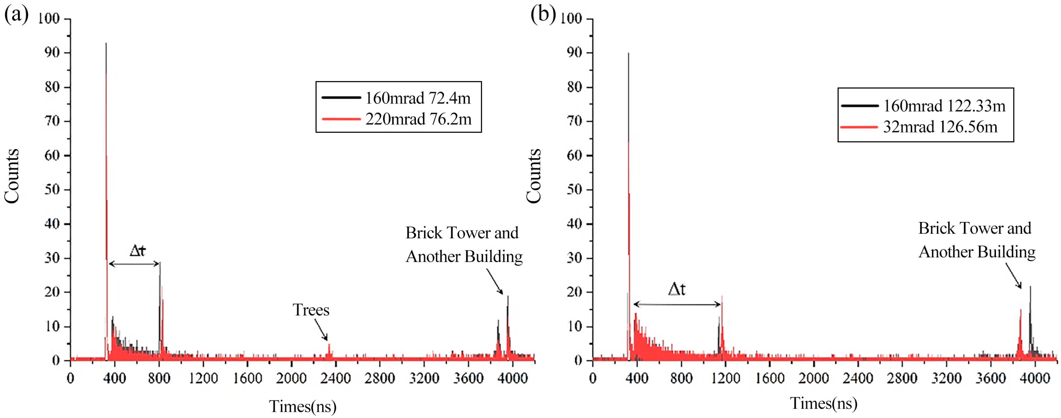
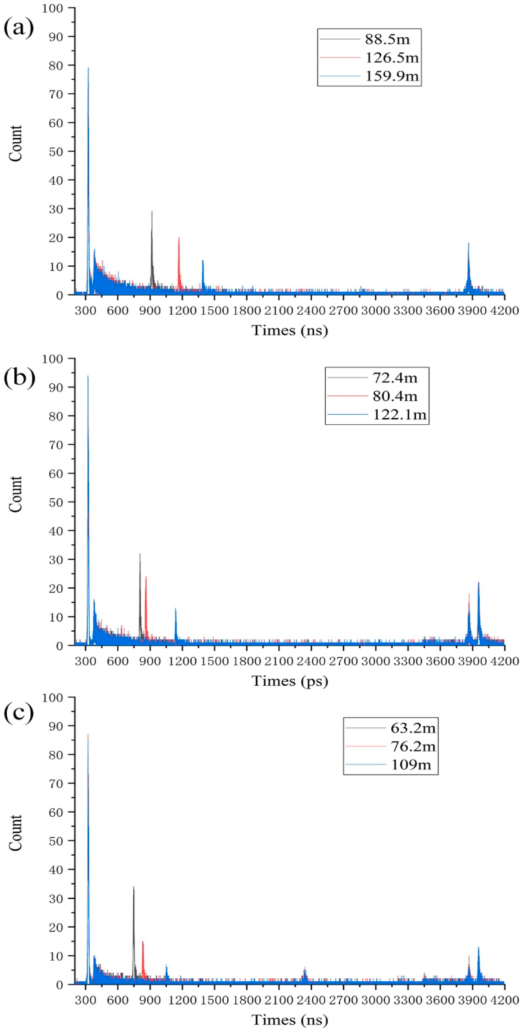
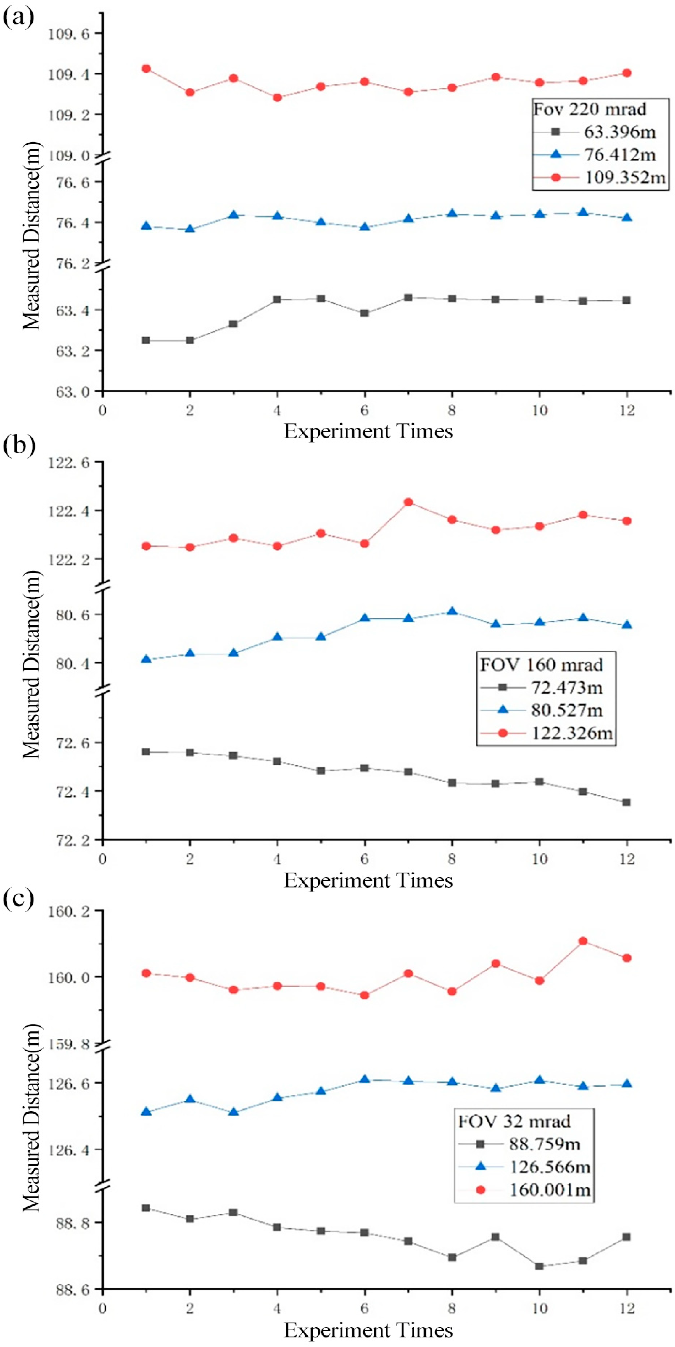
3.2. Experiment and Result

The following experiments were conducted to evaluate the effect of different FOV on the search process. To avoid the influence of the sun and buildings on the investigation, the drone search operations were undertaken in a wild environment at night. The searching system implemented in Figure 1 uses an FT1010 TCSPC module and a SPAD detector. The illumination source is a diode-pumped solid laser at 1064 nm and full width at a half-maximum (FWHM) pulse duration of around 10 ns. The power of the emission laser was fixed at 2.21 W during the experiment. The detection time was fixed at 0.2 s. In order to verify the influence of FOV change on detection, we conducted night drone detection experiments in the open field. Each timing histogram was denoised by a low-pass filter before its peak was located and translated from time to distance.
The experimental setup of the single-photon LiDAR is shown in Figure 1. It is a synchronous scanning searching system. The collimated 1064 nm laser beam was diffused into a circular spot by the laser transmission system. By changing the position of the lens in the laser emission system, the size of the diffused light spot can be controlled. The echoed photons are coupled by the laser receiving system and then focused onto a Si APD-based single-photon detector (SPAD). Additionally, the diameter of the active area of the SPAD was 30 μm. The SPAD was operated in an active quenching, which has a timing jitter of 10 ns and a detection efficiency of 3% at 1064 nm. The histograms were recorded by the time-correlated single photon counting (TCSPC) technique.
Figure 7 shows two UAV echo models at different FOVs at similar distances. Figure 7a shows the counting histogram with FOVs of 160 mrad and 220 mrad, which were targeted toward a target located near 75 m. Figure 7b shows the counting histogram with FOV of 32 mrad and 160 mrad, with targets near 125 m. We used a laser rangefinder to calibrate the target distance and a Gaussian fitting to perform a fit of the echo photon number and obtain the center value of the echo photons. The rightmost part of the image shows the brick tower 540 m away.
When there is cloud cover due to fog, backscatter from atmospheric particles produces a gamma distribution with a high number of photons appearing at the start position of the cloud cover [31]. Since the air humidity at the experimental site is near 70%, we can choose the center of the first backscatter as the timing zero point to calculate the target’s distance from us. The actual distances calculated from the experiments corresponding to Figure 7a are 72.4 m and 76.2 m, and the actual distances calculated from Figure 7b are 122.33 m and 126.56 m. Figure 5 demonstrates the SNR decreases as the FOV increases.
After that, we also conducted search experiments for UAV targets at different distances with the same field of view. To verify the conjectures presented in the previous section, Figure 8 shows the actual photon echoes of the UAV at different distances for three fields of view angles. Figure 8a–c correspond to the FOV of 32 mrad, 160 mrad and 220 mrad, respectively. The unit of the horizontal axis is picoseconds. We can see that the SNR gradually decreases as the distance increases in a low noise environment.
Table 2 shows the results of our multiple search passes at randomly selected locations shown in Figure 8. The results of various experiments show that, for general DJI UAVs, the sub-meter-ranging accuracy can meet UAVs’ search and positioning function.
The detection probability describes the possibility that the searching system can detect the target, and the false alarm rate represents the probability that the searching system mistakenly believes that the target is found due to the noise of the device itself. In order to ensure the good detection performance of the searching system, a fixed threshold K T needs to be set according to the strength of the collected noise signal. Here we set the value of K T to 5. When the accumulated value of the collected laser echo photons and noise photons is greater than the threshold, it is considered an effective detection. When the echo signal and the cumulative value of noise photons are higher than the threshold value, it is regarded as a false alarm detection. Under this threshold condition, the system detection probability P d and false alarm rate P f a can be calculated by Equations (12) and (13), respectively.
P d = 1 k = k T n e N s i g N s i g k K !
P f a = k = k T n e N n o s N n o s k K !
Figure 9 shows some of the specific data involved in the experiment in Figure 8, with each detection time fixed at 0.2 s. Table 3 shows the detection probability and false alarm rate in our drone search experiment corresponding to Figure 8. The detection probability will gradually decrease with the increase of the field of view and the detection distance, and the false alarm rate will also gradually increase.
Due to the limitations of the experimental site, we used a differential algorithm to fit the results of UAV detection, and the fitting goal was for its construction as a quartic inverse proportional function with respect to time. With an SNR threshold of 5, the maximum detection distance can exceed 315 m.
There are several elements not included in the collecting model that may have caused the error in the original experiment:
  • Spectral response of filters: The absorptive BPF used in the experimental measurement does not entirely filter out the corresponding wavelength in the visible region, so the value of background attenuation outside this passband is different and ultimately results in a difference between the received photon and the simulation. It is also worth noting that we avoided the time of noon, so the background noise in the actual experiment was less than in the simulation.
  • Dark count: Our experiments assumed that all photons generated by non-signaled processes are homogeneous “background” processes, but the decay of the incident flux only affects the background count of ambient light and has no effect on the dark count. Although the dark count rate of SPAD is usually low, it can still have an incredible impact on the echo’s signal-to-noise ratio.
  • Target angle: Due to the influence of the weather environment, mainly the wind, the target aircraft cannot be stabilized at a specific position, so it may deviate from the optical axis, resulting in a decrease in the number of echo photons, and also a change in distance, which affects the ranging accuracy in repeated experiments.
It is generally believed that the larger the FOV, the larger the coverage area, the more optical signals received, and the greater the signal strength. In the LiDAR system, a smaller receiving FOV usually leads to suppressed backscattering noise. However, the signal photons suffer great losses due to the small receiving FOV, especially in the Gaussian beam LiDAR. However, through simulation and actual experiments, we found that after the FOV increases, although the received target signal increases, it also strengthens the contribution of multiple scattering to the total received signal. That is, the received background noise is also more significant, especially when the target distance becomes larger.

4. Discussion

The purpose of our manuscript is to investigate the effect of lidar FOV on UAV search results. The method used was the Monte Carlo cycle for single-photon detection. According to the distance of the target and the atmospheric environment, it can be determined that each set of equipment has an optimal field of view. If the largest field of view is selected, the search time can be effectively reduced. In this manuscript, we simulated the atmospheric environment and target distance, which are consistent with previous studies by other researchers [32,33]. The results of the study can provide some ideas for the development of similar lidar. In the simulation stage, the target is also placed in an open field environment. For drones in urban environments, due to the existence of a large number of buildings, the increase in the amount of calculation caused by the multi-entry effect of photons is a problem that many scholars are trying to address. We also conducted a number of calculations on this problem, but did not receive positive results. We aim to undertake in-depth work in this area in the future.
For Figure 4, Figure 5, Figure 6, Figure 7 and Figure 8, Changing the field of view is essentially changing the received noise rate. No matter how the number of echo photons changes, the target detection rate always increases with the decrease of the number of noise photons. The smaller the field of view, that is, the fewer the number of noise photons, the greater the increase gradient of the signal-to-noise ratio as the number of echo photons of a single pulse increases. The gradual increase in the number of noise photons will seriously affect the detection rate of photon counting lidar. As the field of view becomes larger, the target detection rate moves closer to zero.
In our future work, we are considering working on the problem of UAV detection in complex environments and analyzing the impact of multi-return effects on the detection results. At the same time, laser arrays and detector arrays will be used to solve the problem of insufficient spatial resolution, and better filtering methods will be used to ensure that the equipment can work during the day.

5. Conclusions

We suggested and demonstrated a high SNR single-photon lidar system for night environment and analyzed its influence on the detection process under different FOV. Our simulations and data show the existence of a maximum FOV for the search of UAV targets after the SNR threshold is determined. For fast-flying drones, we can detect their location within 0.2 s with a high signal-to-noise ratio. The FOV can be expanded by an order of magnitude in a low noise rate environment at night. The key to the daytime decision search process is noise suppression, including narrower bandwidth filters. For our set of experimental equipment, the maximum field of view can reach 220 mrad for a UAV search mission beyond 100 m.
Overall, our results may provide a new approach for UAV detection as a complement or even an alternative to traditional detection.

Author Contributions

Conceptualization, D.T. and Y.M.; methodology, Z.C. and W.P.; validation, Z.C. and H.Y.; software, W.P. and H.Y.; formal analysis, D.T. and Z.C.; data curation, H.Y.; writing—original draft preparation, Z.C.; writing—review and editing, Z.C.; visualization, H.Y.; supervision, Y.M.; project administration, D.T.; funding acquisition, D.T. All authors have read and agreed to the published version of the manuscript.

Funding

This research was funded by Special Fund of Innovation of China Academy of Engineering Physics, grant number C-2021-CX20210023.

Institutional Review Board Statement

Not applicable.

Informed Consent Statement

Not applicable.

Data Availability Statement

Not applicable.

Conflicts of Interest

The authors declare no conflict of interest.

References

  1. Hammer, M.; Borgmann, B.; Hebel, M.; Arens, M. UAV detection, tracking, and classification by sensor fusion of a 360° lidar system and an alignable classification sensor. In Proceedings of the SPIE 11005, Laser Radar Technology and Applications XXIV, 110050E, Baltimore, MD, USA, 2 May 2019. [Google Scholar]
  2. Klaer, P.; Huang, A.; Sévigny, P.; Rajan, S.; Pant, S.; Patnaik, P.; Balaji, B. An Investigation of Rotary Drone HERM Line Spectrum under Manoeuvering Conditions. Sensors 2020, 20, 5940. [Google Scholar] [CrossRef] [PubMed]
  3. Wagner, W.; Ullrich, A.; Ducic, V.; Melzer, T.; Studnicka, N. Gaussian decomposition and calibration of a novel small-footprint full-waveform digitizing airborne laser scanner. Isprs J. Photogramm. Remote Sens. 2006, 60, 100–112. [Google Scholar] [CrossRef]
  4. Pang, Y.; Zhang, K.; Bai, Z.; Sun, Y.; Yao, M. Design Study of a Large-Angle Optical Scanning System for MEMS LIDAR. Appl. Sci. 2022, 12, 1283. [Google Scholar] [CrossRef]
  5. Wei, Y.S.; Yang, S.L. Analysis and simulation of monopluse radar scanning modes. Syst. Eng. Electron. 2011, 33, 468–472. [Google Scholar]
  6. Chenhao, M.; Yuegang, F.; Ping, G. A composite scanning method and experiment of laser radar. Infrared Laser Eng. 2015, 44, 3270–3272. [Google Scholar]
  7. Guozhu, F.; Huajun, Y.; Qi, Q. Analyzing from simulation of optimizing the spiral scan in the laser radar system. Infrared Laser Eng. 2006, 35, 166–168. [Google Scholar]
  8. Lee, X.; Wang, C.; Luo, Z.; Li, S. Optical design of a new folding scanning system in MEMS-based lidar. Optics Laser Technol. 2020, 125, 106013. [Google Scholar] [CrossRef]
  9. Hadfield, R.H. Single-photon detectors for optical quantum information applications. Nat. Photonics 2009, 3, 696–705. [Google Scholar] [CrossRef]
  10. Buller, G.; Wallace, A. Ranging and Three-Dimensional Imaging Using Time-Correlated Single-Photon Counting and Point-by-Point Acquisition. IEEE J. Sel. Top. Quantum Electron. 2007, 13, 1006–1015. [Google Scholar] [CrossRef] [Green Version]
  11. Ye, L.; Zhang, G.; You, Z. Large-Aperture kHz Operating Frequency Ti-alloy Based Optical Micro Scanning Mirror for LiDAR Application. Micromachines 2017, 8, 120. [Google Scholar] [CrossRef]
  12. Li, Z.-P.; Ye, J.-T.; Huang, X.; Jiang, P.-Y.; Cao, Y.; Hong, Y.; Yu, C.; Zhang, J.; Zhang, Q.; Peng, C.-Z.; et al. Single-photon imaging over 200 km. Optica 2021, 8, 344. [Google Scholar] [CrossRef]
  13. Pearlman, M.R.; Noll, C.E.; Pavlis, E.C.; Lemoine, F.G.; Combrink, L.; Degnan, J.J.; Kirchner, G.; Schreiber, U. The ILRS: Approaching 20 years and planning for the future. J. Geod. 2019, 93, 2161–2180. [Google Scholar] [CrossRef]
  14. Church, P.; Grebe, C.; Matheson, J.; Owens, B. Aerlial and surface security applications using LiDAR. In Proceedings of the SPIE 10636, Laser Radar Teclnology and Applications XXIII, Orlando, FL, USA, 10 May 2018; p. 1063604. [Google Scholar]
  15. Justice, J.; Azzazy, M. Multi-mode LIDAR system for Detecting, Tracking and Engaging Small Unmannedair Vehicles. U.S. Patent 0128922 A1, 10 May 2018. [Google Scholar]
  16. Li, Z.-P.; Huang, X.; Cao, Y.; Wang, B.; Li, Y.-H.; Jin, W.; Yu, C.; Zhang, J.; Zhang, Q.; Peng, C.-Z.; et al. Single-photon computational 3D imaging at 45 km. Photon. Res. 2020, 8, 1532. [Google Scholar] [CrossRef]
  17. Rapp, J.; Ma, Y.; Dawson, R.M.A.; Goyal, V.K. High-flux single-photon lidar. Optica 2021, 8, 30. [Google Scholar] [CrossRef]
  18. Shin, D.; Xu, F.; Venkatraman, D.; Lussana, R.; Villa, F.; Zappa, F.; Goyal, V.K.; Wong, F.N.C.; Shapiro, J.H. Photon-efficient imaging with a single-photon camera. Nat. Commun. 2016, 7, 12046. [Google Scholar] [CrossRef] [PubMed] [Green Version]
  19. Lindell, D.B.; O’Toole, M.; Wetzstein, G. Single-photon 3D imaging with deep sensor fusion. Acm Trans. Graph. 2018, 37, 113:1–113:12. [Google Scholar] [CrossRef]
  20. Cuomo, V.; di Girolamo, P.; Gagliardi, R.V.; Pappalardo, G.; Spinelli, N.; Velotta, R.; Boselli, A.; Berardi, V.; Bartoli, B. Lidar measurements of atmospheric transmissivity. Il Nuovo Cim. C 1995, 18, 209–222. [Google Scholar] [CrossRef] [Green Version]
  21. Redington, R.W. Elements of infrared technology: Generation, transmission and detection. Solid State Electron. 1962, 5, 361–363. [Google Scholar] [CrossRef]
  22. Kim, I.I.; Mcarthur, B.; Korevaar, E.J. Comparison of laser beam propagation at 785 nm and 1550 nm in fog and haze for optical wireless communications. Proc. Spie Int. Soc. Opt. Eng. 2001, 4214, 26–37. [Google Scholar]
  23. Al Naboulsi, M.C.; Sizun, H.; de Fornel, F. Fog attenuation prediction for optical and infrared waves. Opt. Eng. 2004, 43, 319. [Google Scholar] [CrossRef]
  24. Grabner, M.; Kvicera, V. The wavelength dependent model of extinction in fog and haze for free space optical communication. Opt. Express 2011, 19, 3379–3386. [Google Scholar] [CrossRef] [PubMed]
  25. Zhai, D.S.; Fu, H.L.; He, S.H. Study on the characteristic of laser ranging based on diffuse reflection. Astron. Res. Technol. 2009, 6, 13–19. [Google Scholar]
  26. Liu, Z.X.; Li, X.J.; Fan, X.J. Measurement technology study of laser target reflection characteristic. Electro-Opt. Technol. Appl. 2007, 22, 46–47. [Google Scholar]
  27. Liu, Z.; Hunt, W.; Vaughan, M.; Hostetler, C.; McGill, M.; Powell, K.; Winker, D.; Hu, Y. Estimating random errors due to shot noise in backscatter lidar observations. Appl. Opt. 2006, 45, 4437–4447. [Google Scholar] [CrossRef] [PubMed]
  28. Boutabba, N.; Grira, S.; Eleuch, H. Atomic population inversion and absorption dispersion-spectra driven by modified double-exponential quotient pulses in a three-level atom. Results Phys. 2021, 24, 104108. [Google Scholar] [CrossRef]
  29. Méjean, G.; Kasparian, J.; Yu, J.; Frey, S.; Salmon, E.; Wolf, J.P. Remote detection and identification of biological aerosols using a femtosecond terawatt lidar system. Appl. Phys. B 2004, 78, 535–537. [Google Scholar] [CrossRef]
  30. Cornette, W.M.; Shanks, J.G. Physically reasonable analytic expression for the single-scattering phase function. Appl. Opt. 1992, 31, 3152–3160. [Google Scholar] [CrossRef]
  31. Patanwala, S.M.; Gyongy, I.; Mai, H.; Aßmann, A.; Dutton, N.A.W.; Rae, B.R.; Henderson, R.K. A High-Throughput Photon Processing Technique for Range Extension of SPAD-Based LiDAR Receivers. IEEE Open J. Solid-State Circuits Soc. 2022, 2, 12–25. [Google Scholar] [CrossRef]
  32. Pasquinelli, K.; Lussana, R.; Tisa, S.; Villa, F.; Zappa, F. Single-photon detectors modelling and selection criteria for high-background LiDAR. IEEE Sens. J. 2020, 20, 7021–7032. [Google Scholar] [CrossRef]
  33. Starkov, A.V.; Noormohammadian, M.; Oppelug, U.G. A stoclastic model and a variance-reduction Monte-Carlo method for the calculation of light transport. Appl. Phys. B 1995, 60, 335–340. [Google Scholar] [CrossRef]
Figure 1. Schematic of the experimental setup for UAV detection. Moreover, a band-pass filter (BPF) is set in front of the lens to operate the photons reflected from the UAVs. The photons are then focused by a lens onto the SPAD.
Photonics 09 00972 g001
Figure 2. Laser transmission and receiving systems.
Photonics 09 00972 g002
Figure 3. Monte Carlo method for detection.
Photonics 09 00972 g003
Figure 4. Photon echoes in different fields of view under daylight conditions. The field of view Angle in the simulation is (a)1.2mrad, (b) 1.0mrad, (c) 0.9 mrad, (d) 0.8 mrad, (e) 0.6 mrad, and (f) 0.5 mrad.
Photonics 09 00972 g004
Figure 5. Photon echoes in different fields of view (a) 40 mrad, (b) 30 mrad, (c) 25 mrad, and (d) 20 mrad under nighttime conditions.
Photonics 09 00972 g005
Figure 6. At the FOV of 32 mrad, the UAV was located at (a) 450 m, (b) 500 m, (c) 550 m, (d) 600 m.
Photonics 09 00972 g006
Figure 7. Search experiment at similar distances with different fields of view. (a) FOVs of 160 mrad and 220 mrad, which the target located near 75 m. (b) FOV of 32 mrad and 160 mrad, which targets near 125 m.
Photonics 09 00972 g007
Figure 8. Search experiments with FOVs of (a) 32 mrad, (b) 160 mrad, (c) 220 mrad.
Photonics 09 00972 g008
Figure 9. Search data with FOVs of (a) 220 mrad, (b) 160 mrad, (c) 32 mrad.
Photonics 09 00972 g009
Table 1. Comment parameters for the detection system.
ParameterComment
Laser systemOnda 1064 nm, bright solution
Illumination wavelength1064 nm
Laser Repetition rate60 KHz
Average power2.59 W
DetectorsSPD500, Silicon Single Photon Avalanche Diode Detector
Histogram length65535 bin
Bin width~64 ps
Table 2. Detection results at different distances and fields of view.
FOVCalibrated DistanceMeasured DistanceErrorVariance
88.5 m88.759 m0.259 m0.060
32 mrad126.5 m126.566 m0.066 m0.001
159.9 m160.001 m0.101 m0.002
72.4 m72.473 m0.073 m0.004
160 mrad80.4 m80.527 m0.127 m0.090
122.1 m122.326 m0.226 m0.004
63.2 m63.396 m0.196 m0.006
220 mrad76.2 m76.412 m0.212 m0.001
109 m109.352 m0.352 m0.002
Table 3. Detection probability and false alarm rate at different distances and fields of view.
FOVMeasured DistanceSNRDetection ProbabilityFalse Alarm Rate
88.759 m2799.99%0.327%
32 mrad126.566 m2099.99%0.301%
160.001 m1699.90%0.380%
72.473 m2999.99%0.299%
160 mrad80.527 m2599.99%0.309%
122.326 m1298.72%0.352%
63.396 m3399.99%0.283%
220 mrad76.412 m1899.97%0.301%
109.352 m993.92%0.366%
Publisher’s Note: MDPI stays neutral with regard to jurisdictional claims in published maps and institutional affiliations.

