Enhancement of Imaging Quality of Interferenceless Coded Aperture Correlation Holography Based on Physics-Informed Deep Learning

Abstract

Interferenceless coded aperture correlation holography (I-COACH) was recently introduced for recording incoherent holograms without two-wave interference. In I-COACH, the light radiated from an object is modulated by a pseudo-randomly-coded phase mask and recorded as a hologram by a digital camera without interfering with any other beams. The image reconstruction is conducted by correlating the object hologram with the point spread hologram. However, the image reconstructed by the conventional correlation algorithm suffers from serious background noise, which leads to poor imaging quality. In this work, via an effective combination of the speckle correlation and neural network, we propose a high-quality reconstruction strategy based on physics-informed deep learning. Specifically, this method takes the autocorrelation of the speckle image as the input of the network, and switches from establishing a direct mapping between the object and the image into a mapping between the autocorrelations of the two. This method improves the interpretability of neural networks through prior physics knowledge, thereby remedying the data dependence and computational cost. In addition, once a final model is obtained, the image reconstruction can be completed by one camera exposure. Experimental results demonstrate that the background noise can be effectively suppressed, and the resolution of the reconstructed images can be enhanced by three times.

1. Introduction

Indirect imaging techniques using coded aperture masks have gained intensive attentions due to their capability of improving the depth of field, the field of view, and practicability over conventional imaging systems [1,2]. Digital holography is an indirect imaging technique where holograms are first acquired using an image sensor, and then the image is reconstructed digitally by a computational algorithm [3,4]. An efficient, rapid, and well-established method is the coded aperture correlation holography (COACH) [5,6]. Originally, COACH was invented as an incoherent, self-interference imaging technique. Unlike other coded aperture imaging systems such as FINCH [7,8], COACH uses a pseudo-randomly-coded phase mask (CPM) instead of a quadratic phase mask. Thus, a CPM modulates the light field as an axial-resolution enhancer. Moreover, the lateral and axial resolutions of COACH turn out to be comparable with those of ordinary imaging systems. Apparently, in coded aperture imaging systems, the three-dimensional (3D) position of the object is encoded not only in the phase but also in the amplitude, which is modulated by the CPM. Therefore, COACH has the capability of imaging a 3D object without two-wave interference. Such an improved vision of COACH is termed interferenceless COACH (I-COACH) [9]. In this system, the optical configuration is simplified due to the interferenceless feature, and the imaging efficiency is increased. Recently, Hai et al. converted the I-COACH technology into coherent imaging systems [10]. In this method, a special CPM modulates the system’s PSF to be randomly and sparsely distributed dots [11,12]. It should be noted that image reconstruction is realized by the cross-correlation algorithm between the object hologram and the point spread hologram of the system. When the width of the autocorrelation of the point spread hologram is narrow enough, the object can be reconstructed reliably. Nevertheless, the autocorrelation of a point spread hologram contains a lot of noise, which is the main reason for the inherent background term. To achieve high-quality reconstruction, several techniques have been proposed to reduce the noise. For example, in the phase-filtered method [13,14], the signal-to-noise ratio (SNR) is improved by a cross-correlation between the object hologram and the phase-only filtered version of the point spread hologram. However, this method requires multiple exposures to obtain point spread holograms and object holograms, resulting in a reduced imaging speed. In contrast, the non-linear filtering method [15] requires one camera exposure and multiple iterations to complete the reconstruction. Recently, some researchers have proposed an optimization scheme [16] that requires only one exposure and one reconstruction. However, it improves the temporal resolution at a moderate sacrifice of SNR. Therefore, further improvements are demanded to make this technology more practical.

In recent years, with the advent of digital technology, big data and advanced optoelectronic technology, deep learning has shown great potential in solving various optical imaging problems, including wave-front sensing [17], super-resolution imaging [18,19], noise reduction [20], digital holography imaging [21,22,23,24,25], optical tomography imaging [26,27], etc. As a typical inverse problem, deep learning has also been utilized in the scattering imaging, where the light from the target object is scattered, and a speckle image is obtained. The goal of learning is to establish the mapping between the speckle image and the target image by building highly generalizable networks. Shuai et al. proposed the IDiffNet method and investigated its performance in different cases [28]. Yang et al. trained a deep neural network [29] by 1000 pairs of speckle images via multimode fibers and 2000 pairs of speckle images via glass diffusers. These methods solve the problems by purely data-driven techniques. However, they suffer from some drawbacks. First, deep learning cannot offer the same interpretability, flexibility, versatility, and reliability as the conventional model-based methods. Intrinsic information can hardly be extracted under highly degenerating conditions, leading to a limited generalization capability. Second, deep learning methods need to tune and train a huge number of parameters, resulting in unaffordable computational costs.

In this paper, aided by the physics prior [30] of scattering, a physics-informed deep learning method is proposed for image reconstruction in the I-COACH system under coherent illumination. On one hand, a PSF is the response of those object points located at a specific z plane. Thus, the light from those object points outside this specific axial region is out of focus on the camera plane, and the resulting PSFs associated with those points cannot restore images with acceptable quality. For better understanding, it is necessary to stress that the proposed strategy seeks to improve the reconstruction quality and resolution in the two-dimensional imaging, while the 3D case is not of main concern in this paper. On the other hand, this method can break through the limitations and improve the image quality thanks to CNN’s powerful capabilities in solving inverse imaging problems, as demonstrated in the experimental section. The methodology is introduced in Section 2. The experiments are discussed in the Section 3, followed by the conclusion in the Section 4.

2. Methodology

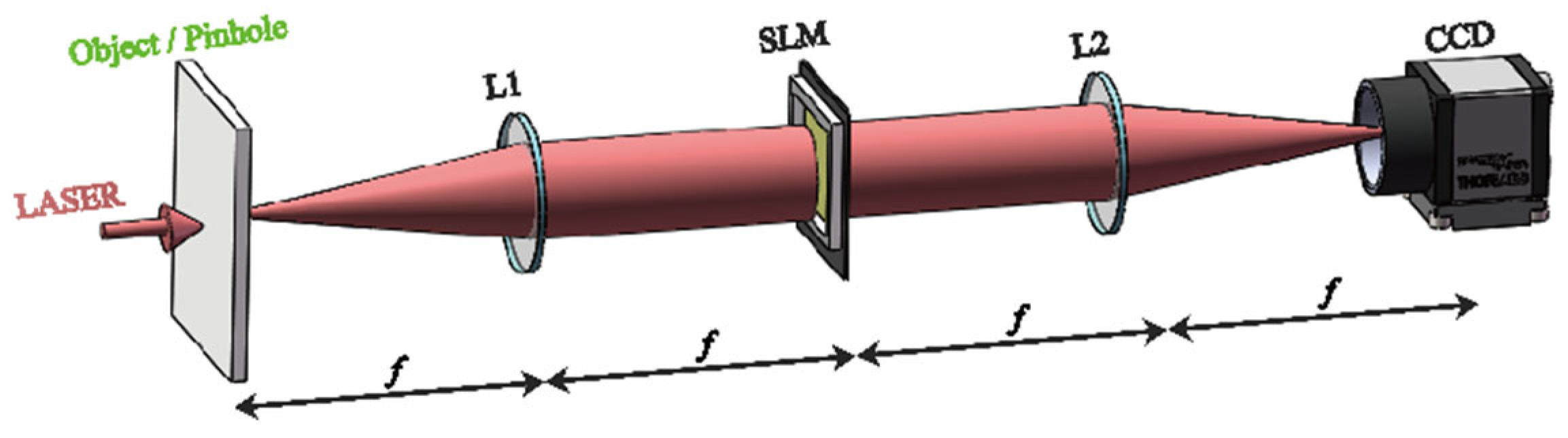
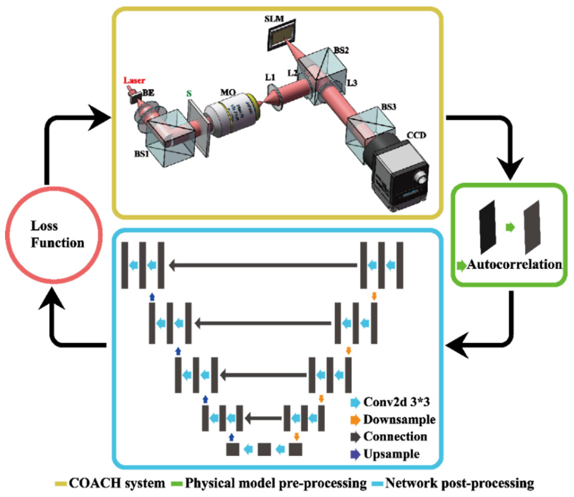
2.1. Coherently Illuminated I-COACH

Wave propagation through an inhomogeneous scattering medium will generate a pattern of fluctuating intensities, maintaining the same physics law in different transmitted modes. The speckle correlation theory and optical memory effect in wave transmission through disordered media can be employed to analyse the shift-invariance of speckle patterns [31,32,33]. Due to the randomness properties of the CPM, the I-COACH can be considered as scattering imaging. Following Ref. [10], by designing the PSF to be randomly and sparsely distributed dots, the I-COACH technology can be extended from incoherent to coherent imaging systems by utilizing a coherent illumination. Thus, a hologram H_OBJ at the image plane is represented as,

$$\begin{array}{l}{H}_{OBJ}={\left|A\left(\overline{r}\right)\ast {\displaystyle \sum _k{a}_k\delta \left(\overline{r}-{\overline{r}}_k\right)}\right|}^2={\left|{\displaystyle \sum _k{a}_k}A\left(\overline{r}-{\overline{r}}_k\right)\right|}^2\\ ={\displaystyle \sum _k{\left|a_k\right|}^2}{\left|A\left(\overline{r}-{\overline{r}}_k\right)\right|}^2={\left|A\left(\overline{r}\right)\right|}^2\ast {\displaystyle \sum _k{\left|a_k\right|}^2}\delta \left(\overline{r}-{\overline{r}}_k\right)\end{array}$$

(1)

where * denotes convolution, $\overline{r}=(x,y)$ is the abscissa coordinate, $A\left(\overline{r}\right)$ is the complex amplitude, δ(•) is the Dirac function, k is the dot index in the CPM and a_k is a complex-valued constant. ${\displaystyle \sum _k{a}_k\delta \left(\overline{r}-{\overline{r}}_k\right)}$ is the PSF of the optical system and ${\displaystyle \sum _k{\left|a_k\right|}^2}\delta \left(\overline{r}-{\overline{r}}_k\right)$ is regarded as the point spread hologram H_PSF. Specifically, the optical configuration of the coherent I-COACH is a classical 4F spatial filtering system, as shown in Figure 1. The light emitted from the object is Fourier transformed by lens L₁. Then, the spatial spectrum of the object is modulated by a pseudo-random CPM displayed on a spatial light modulator (SLM). The light passes through the lens L₂ and then achieves the camera plane.

Therefore, image reconstruction is carried out by the cross-correlation between H_OBJ and H_PSF as follows,

$$\begin{array}{l}{I}_{IMG}=H_{OBJ}\otimes H_{PSF}={\left|A\left(\overline{r}\right)\ast {\displaystyle \sum _k{a}_k\delta \left(\overline{r}-{\overline{r}}_k\right)}\right|}^2\otimes H_{PSF}\\ ={\left|A\left(\overline{r}\right)\right|}^2\ast {\displaystyle \sum _k{a}_k{}^2\delta \left(\overline{r}-{\overline{r}}_k\right)}\otimes H_{PSF}\\ ={\Im }^{-1}\left\{\Im \left[{\left|A\left(\overline{r}\right)\right|}^2\right]h^2\exp \left(j\phi \right)\exp \left(-j\phi \right)\right\}\\ ={\left|A\left(\overline{r}\right)\right|}^2\ast {\Im }^{-1}\left\{h^2\right\}\approx O\left(\overline{r}\right)\end{array}$$

(2)

where $\otimes$ represents the correlation operator, $\Im (·)$ stands for the two-dimensional Fourier transform. Then, we have $\Im \left\{{\displaystyle \sum _k{a}_k{}^2\delta \left(\overline{r}-{\overline{r}}_k\right)}\right\}=h\exp \left(j\phi \right)$, where h and φ denote the amplitude and phase of the Fourier transform of the PSF, respectively. The approximation of Equation (2) is valid under the assumption that the reconstructing function ${\Im }^{-1}\left\{h^2\right\}$ is a sharply peaked function, which is true for randomly distributed dots [12].

According to the speckle correlation theory, the object can also be alternatively reconstructed by the autocorrelation of H_OBJ

$$\begin{array}{l}{H}_{OBJ}\otimes H_{OBJ}={\left|A\left(\overline{r}\right)\ast {\displaystyle \sum _k{a}_k\delta \left(\overline{r}-{\overline{r}}_k\right)}\right|}^2\otimes {\left|A\left(\overline{r}\right)\ast {\displaystyle \sum _k{a}_k\delta \left(\overline{r}-{\overline{r}}_k\right)}\right|}^2\\ =\left({\left|A\left(\overline{r}\right)\right|}^2\otimes {\left|A\left(\overline{r}\right)\right|}^2\right)\ast \left({\displaystyle \sum _k{a}_k{}^2\delta \left(\overline{r}-{\overline{r}}_k\right)}\otimes {\displaystyle \sum _k{a}_k{}^2\delta \left(\overline{r}-{\overline{r}}_k\right)}\right)\end{array}$$

(3)

where $\left({\displaystyle \sum _k{a}_k{}^2\delta \left(\overline{r}-{\overline{r}}_k\right)}\otimes {\displaystyle \sum _k{a}_k{}^2\delta \left(\overline{r}-{\overline{r}}_k\right)}\right)$ is a sharply peaked function [31] representing the autocorrelation of H_PSF. Therefore, the right-handed side of Equation (3) is approximately equal to the autocorrelation of the object with an additional constant background term C [32]. Thus, Equation (3) can be further simplified as

$$H_{OBJ}\otimes H_{OBJ}=\left({\left|A\left(\overline{r}\right)\right|}^2\otimes {\left|A\left(\overline{r}\right)\right|}^2\right)+C.$$

(4)

According to the Wiener–Khinchin theorem [34], the autocorrelation of a speckle image equals the inverse Fourier transform of its power density spectrum. The mathematical operation can be expressed as

$$H_{OBJ}\otimes H_{OBJ}={\Im }^{-1}\left\{{\left|\Im \left(H_{OBJ}\right)\right|}^2\right\}.$$

(5)

Hence, when the autocorrelation of H_OBJ is calculated first, the autocorrelation of the object can be obtained by subtracting the background term C. Then, the Fourier amplitude of the object can be calculated as,

$$\left|\Im \left(O\right)\right|=\sqrt{\left|\Im \left(H_{OBJ}\otimes H_{OBJ}\right)\right|}.$$

(6)

The object’s phase information can then be obtained using some iterative phase-retrieval algorithms, e.g., the Gerchberg–Saxton (GS) algorithm [35,36]. In general, the cross-correlation algorithm and autocorrelation algorithm are both based on the speckle correlation theory. In the cross-correlation method, H_OBJ and H_PSF should be recorded in advance for reconstruction. The autocorrelation method does not need to provide H_PSF, but it cannot conduct reconstruction without specifying the background term C. In addition, both methods require the width of the autocorrelation of H_PSF to be small enough to guarantee the reconstruction quality. In practice, however, the autocorrelation of H_PSF contains a large amount of noise, which is the main reason for the background noise, resulting in a low image quality.

2.2. Numerical Analysis

The intrinsic connection among different CPMs is investigated subsequently. Seven different CPMs, namely CPM1 to CPM7, are generated by the GS algorithm, which sparsifies the PSF into 20, 30, …, and 80 dots, respectively. In the first case, speckle images are captured through different CPMs for the same object. It is necessary to verify whether these speckle images are similar. Therefore, the cross-correlations between the speckle images associated with different CPMs and that associated with CPM4 are calculated, respectively. The results are shown in Figure 2. It can be found that the correlation of different speckle images is irregular, and there is almost no similarity between the speckle images associated with different CPMs. In the second case, an object “3” is used as an example to verify the similarity between the autocorrelation of the speckle image and the autocorrelation of the object, as shown in Figure 3. The autocorrelations are calculated for the speckle images modulated by different CPMs. The autocorrelation of the object is highly similar to that of the speckles, and the relative difference between them lies in the background term. Therefore, Figure 3 verifies that the derivation in Equation (4) is correct. In the third case, to demonstrate the similarity between the autocorrelations of the speckle images associated with different objects, all the objects are modulated by CPM4. Figure 4 shows the simulation results. Because the energy is mainly concentrated in the central region, the autocorrelations of speckle images have a conspicuous crest. However, by enlarging Figure 4a, it can be observed from Figure 4b that their respective details are different. Therefore, it can be confirmed that the autocorrelations of the speckle images associated with different objects via the same CPM have no similarity.

It also can be found from Figure 3 that the magnitude of the background term depends mainly on the sparsity of the object. Different CPMs modulate the same object sequentially so that the object becomes increasingly sparse. Subsequently, the intensity of the corresponding background term becomes larger. Although CPM makes the intensity of the background term different, the trend of the background term is consistent for the same object. Contrary to this, Figure 4 modulates four different objects with the same CPM, and it is evident that the intensities of the respective background terms are different, and the changing trends are significantly different. It implies that the background term C is mainly determined by the object itself, but less relevant to the modulating CPM.

2.3. Image Reconstruction by Physics-Informed Deep Learning

In a typical data-driven deep learning method, imaging is treated as a mapping problem from massive labeled data,

$$P_{learn}=\arg \min {\displaystyle \sum _{i}L\left[P\left(x_i\right),y_i\right]}.$$

(7)

where a speckle image x_i and its corresponding ground truth object y_i form a pair, and P is the mapping between x_i and y_i. Thus, P_learn is the obtained optimal approximation of the operation, P. L is the loss function for error metrics, which is to be minimized by optimization. However, the purely data-driven deep learning method faces several challenges, such as resource waste, dimensional disaster, etc. To overcome the drawbacks of data-driven deep learning methods, it is preferred to make full use of physics priors in the COACH imaging. A new framework is designed in Figure 5. It consists of a physics model-based pre-processing module and a network-based post-processing module. According to Equation (4), the autocorrelation of a speckle image is linked to the autocorrelation of the object. Therefore, the autocorrelation function is substituted into the former module as a physical model. Then the calculated result of the former module is substituted into the latter module for training. The pattern displayed by the SLM or a physical object located there is taken as the ground truth.

This framework switches from establishing a direct mapping between the speckle image and ground truth into a mapping between the autocorrelations of the two. Thus, the objective function of Equation (7) can be rewritten as follows

$$P_{learn}=\arg \min {\displaystyle \sum _{i}L\left[P\left(x_i\otimes x_i\right),y_i\otimes y_i\right]}.$$

(8)

Interestingly, as the background term C is only determined by the object x_i, but less relevant with the scattering media, the training space is greatly reduced by adapting the mapping function P from x_i to y_i into that from $x_i\otimes x_i$ to $y_i\otimes y_i$. Adding valid physics priors can reduce the dimensionality of variables to be trained in the network model, in which case the dimension disaster arising in the conventional end-to-end training is remedied, and the reliability of the trained results can be significantly improved. Therefore, given the same set of samples, the proposed method can significantly reduce the imaging error. In the neural network-based post-processing module, a typical network named UNet [37,38] is utilized for training P_learn. UNet is simple, efficient and easy to be built, and it can be trained using small data sets. It consists of a down-sampling path as well as a symmetric up-sampling path. The former takes the autocorrelation of speckle images as an input, and the latter outputs a trained image. We adopt four types of modules, namely convolution blocks (3 × 3 convolution + batch normalization + Leaky ReLU), max-pooling blocks (2 × 2), up-convolution blocks (3 × 3 de-convolution + batch normalization + Leaky ReLU) and skip connection blocks, respectively. A loss function consisting of a negative Pearson correlation coefficient (NPCC) [39] and the mean square error (MSE) is used. The NPCC loss ranging between −1 and 1 guarantees linear amplification and bias-free reconstruction, which increases the convergence probability. A negative value represents a negative correlation, and vice versa. The loss function can be formulated as

$$L=L_{NPCC}+L_{MSE}.$$

(9)

with $L_{NPCC}=\frac{-{\displaystyle \sum _{x=1}^w{\displaystyle \sum _{y=1}^b\left[i(x,y)-\widehat{i}\right]\left[I(x,y)-\widehat{I}\right]}}}{\sqrt{{\displaystyle \sum _{x=1}^w{\displaystyle \sum _{y=1}^b{\left[i(x,y)-\widehat{i}\right]}^2\sqrt{{\displaystyle \sum _{x=1}^w{\displaystyle \sum _{y=1}^b{\left[I(x,y)-\widehat{I}\right]}^2}}}}}}}$ and $L_{MSE}={\displaystyle \sum _{x=1}^w}{\displaystyle \sum _{y=1}^b}{\left|\tilde{i}(x,y)-I(x,y)\right|}^2$.

Here $\widehat{I}$ and $\widehat{i}$ are the mean value of the ground truth intensity I and that of the output i, respectively, and $\tilde{i}$ is a normalized image of i. The combined loss function has an excellent capability in reconstructing objects with complexity through scattering media [40].

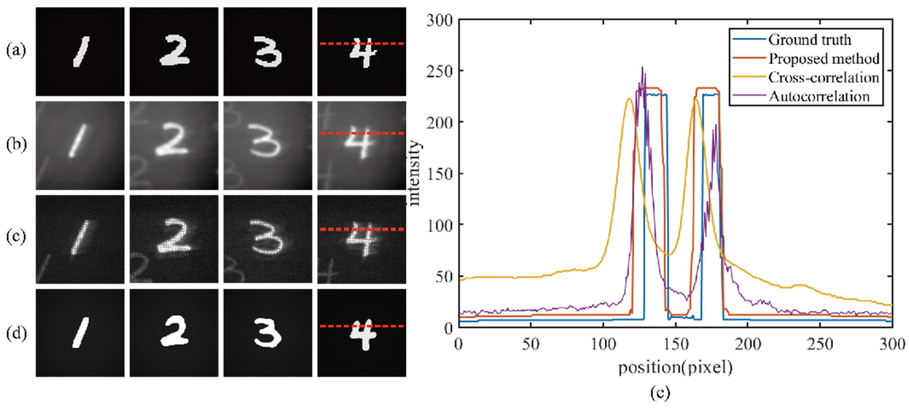
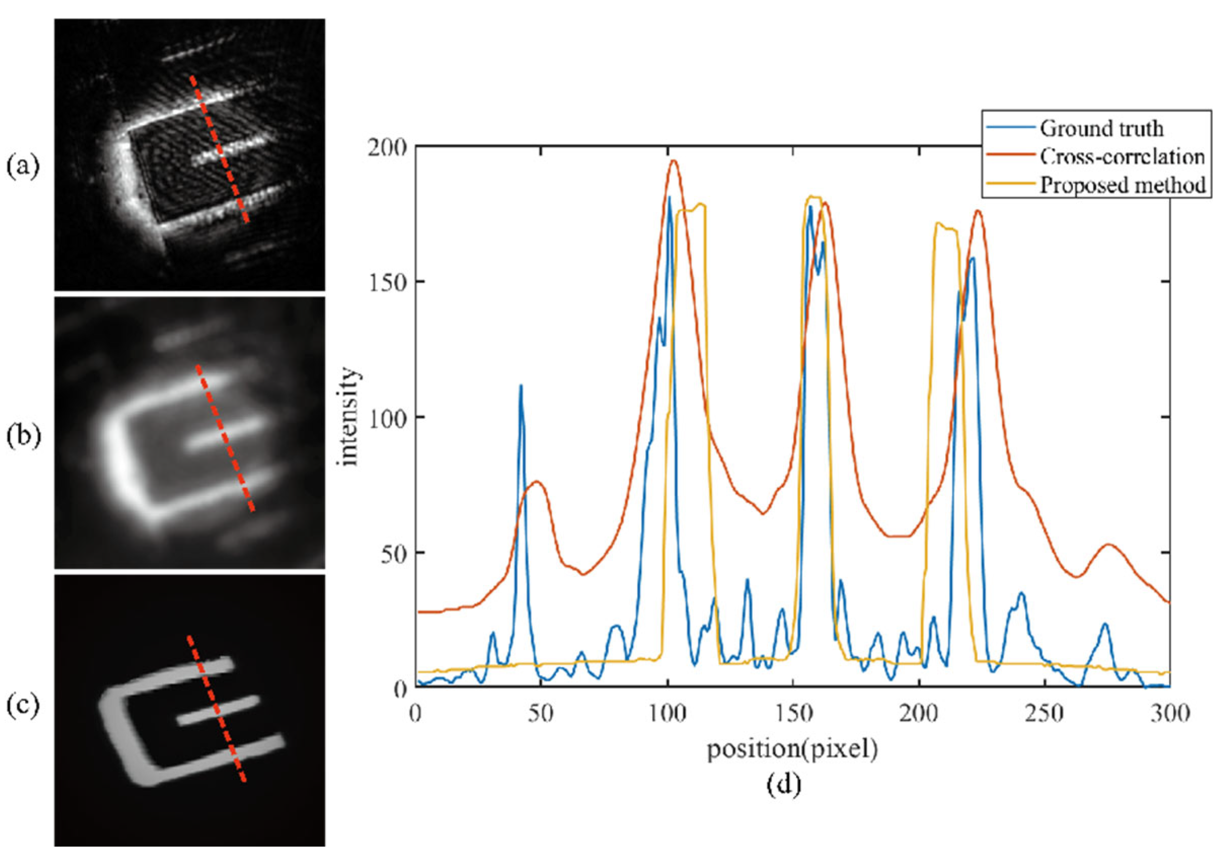
3. Experimental Results and Discussions

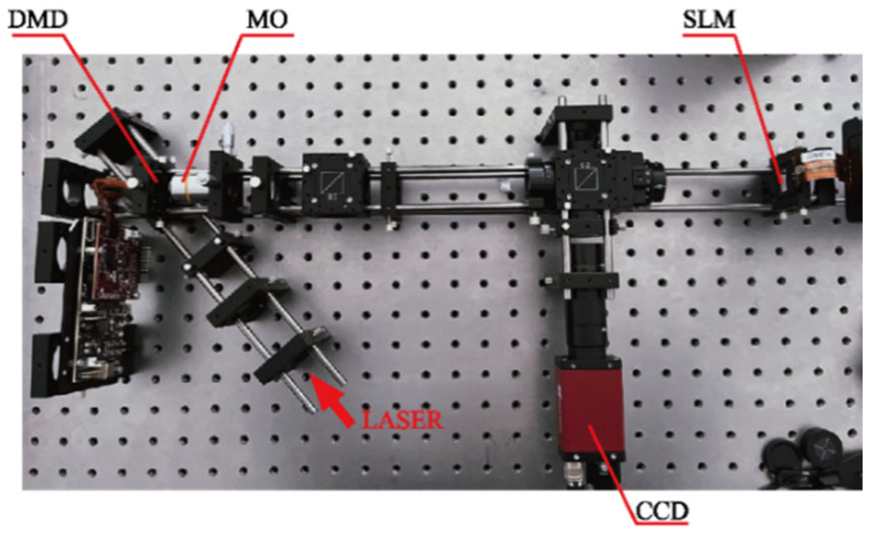
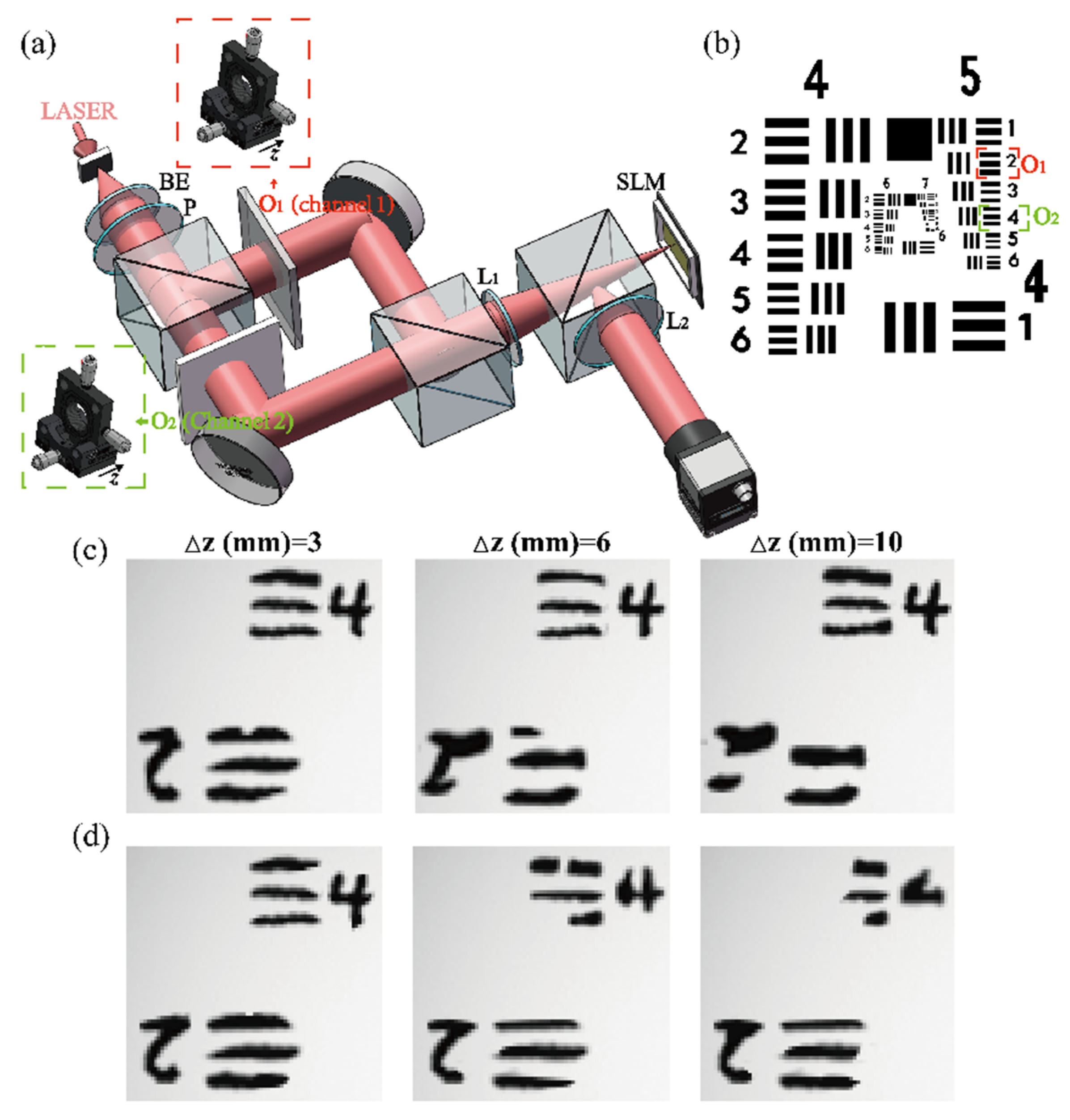
3.1. Experimental Design

The experimental setup is illustrated in Figure 6. A He-Ne laser with a maximum output power of 41 mW and λ = 632.8 nm was adopted as the light source. A digital micromirror device (DMD) with 1920×1080 pixels and a pixel size of 7.56 μm and a microscope objective OLYMPUS MPLFLN10X with a numerical aperture of 0.25 were adopted. An SLM HOLOEYE PLUTO with a resolution of 1920 × 1080 pixels displayed the CPM and a camera Manta G-419 with a resolution of 2048 × 2048 pixels captured the images. In addition, three lenses L₁, L₂ and L₃ with focal lengths of 60 mm, 125 mm, and 125 mm, respectively, all with an aperture size of 25.4 mm, were utilized. An Adam [41] optimizer was selected to update the weights in the network training process. All the algorithms were run on the same workstation with an i5-10400F CPU (2.9 GHz). In particular, a GPU NVIDIA GeForce RTX 2060 was used for the running the program.

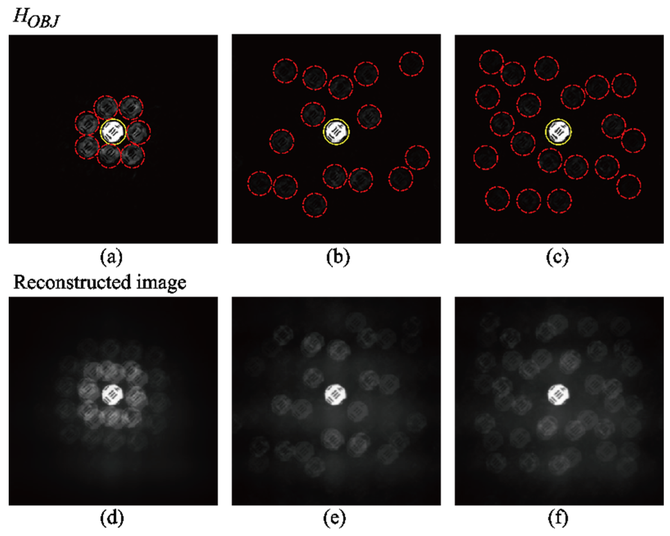
3.2. Determine the Optimal Number of Dots

The optimal number of dots was determined first. We placed a USAF 1951 resolution chart at the object plane, in which Element 4 of Group 6 (G6, E4) was chosen in the resolution chart as a target object. The light modulated by different CPMs was utilized to generate H_PSF composed of different numbers of dots. According to the actual system configuration, we chose H_PSF containing 8 dots, 15 dots, and 20 dots, respectively. Figure 7a–c shows the recorded holograms, in which case a special H_PSF is designed so that the image of the object is convolved with an array of isolated dots. Henceforth the number and distribution of the dots directly determine those of the image replications. The distance between any two adjacent dots should be greater than the object to avoid overlapping between different image replications. The red solid-line circles indicate the resulting H_OBJ contains multiple duplicated images of the target object. It can be found that the more dots contained, the lower the intensity is allocated to each dot, resulting in a darker hologram. In addition, the yellow circle indicates the signal from the unmodulated part of the CPM. Figure 7d–f illustrates their corresponding reconstruction images. To conduct a reliable comparison, we evaluated the quality of each image in terms of SNR and structure similarity index measure (SSIM), as presented in

Table 1. Comparison of the reconstructed images for different H_PSF.

Dot Number	8	15	20
SNR (dB)	12.09	12.94	11.08
SSIM	0.47	0.49	0.42

. It can be found that the number of duplicated images on the camera plane has significant implications on the reconstructed image quality. Too many replications of the object reduce the SNR level of the reconstructed images. At the same time, an H_PSF consisting of fewer dots increases the out-of-focus image intensity and blurs the reconstructed images. A H_PSF containing 15 dots is preferred.

3.3. Data Collection and Implementation Details

The objects were mainly chosen from the MNIST dataset, Fashion-MNIST dataset [42], and the USAF 1951 resolution chart. Samples were randomly selected from the MNIST dataset containing 500 single characters and 500 double-character objects, respectively. The resolution chart dataset contains 470 images obtained by cutting different parts of the USAF image. To test more complicated cases, 500 images were randomly chosen from the Fashion-MNIST dataset, which has more abundant detailed features. All the training datasets were displayed on the DMD for collecting the input images and their corresponding ground truths. Then, data enhancement like rotating, overturning, resizing, etc. is implemented, and 11820 speckle images were obtained. The speckle autocorrelations were calculated based on Equation (5). A central area of 300 × 300 pixels was extracted from the speckle autocorrelations, forming the training datasets, and fed into the neural network. The whole training program took about 3 h.

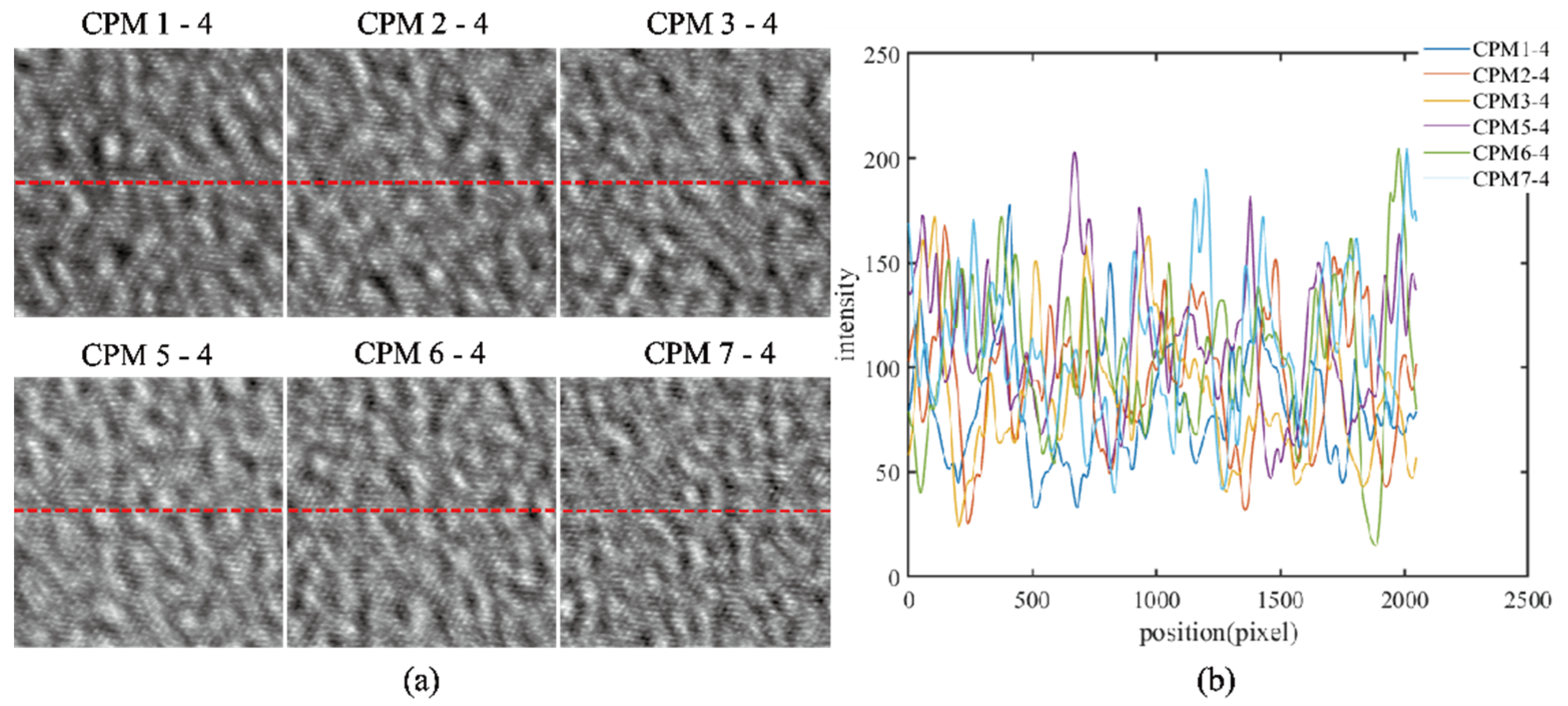
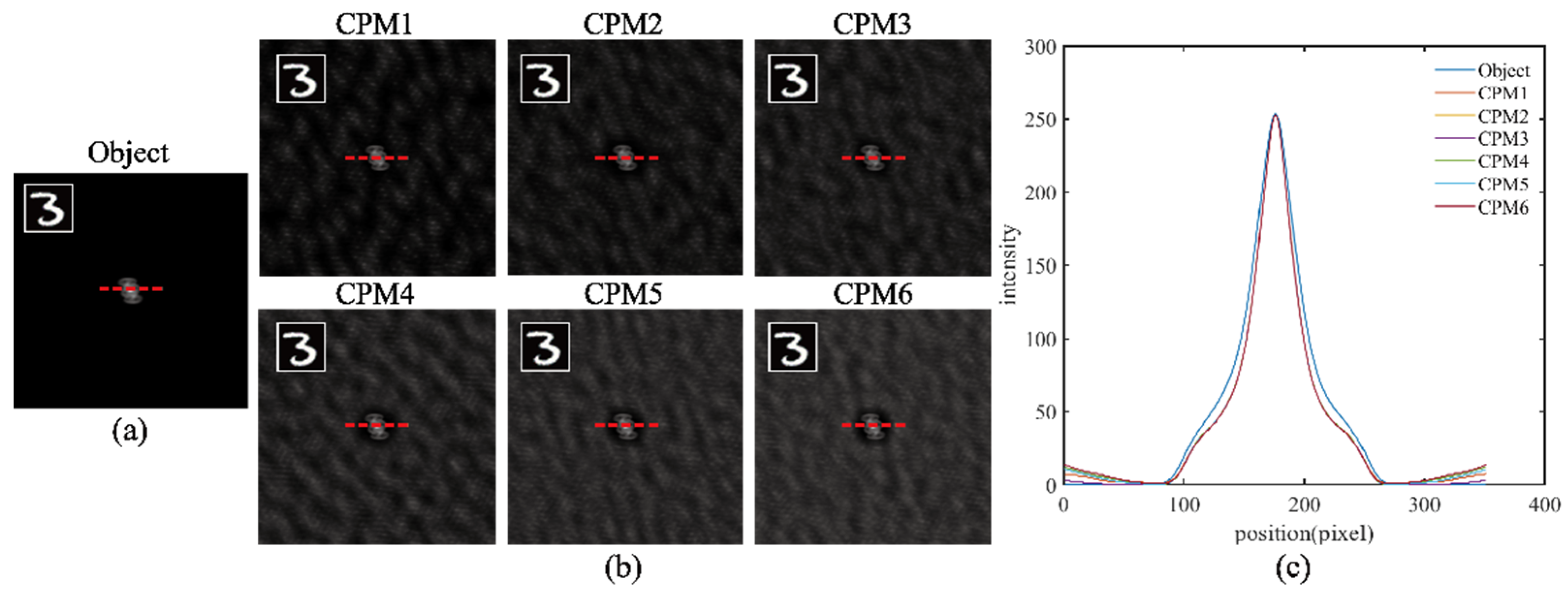
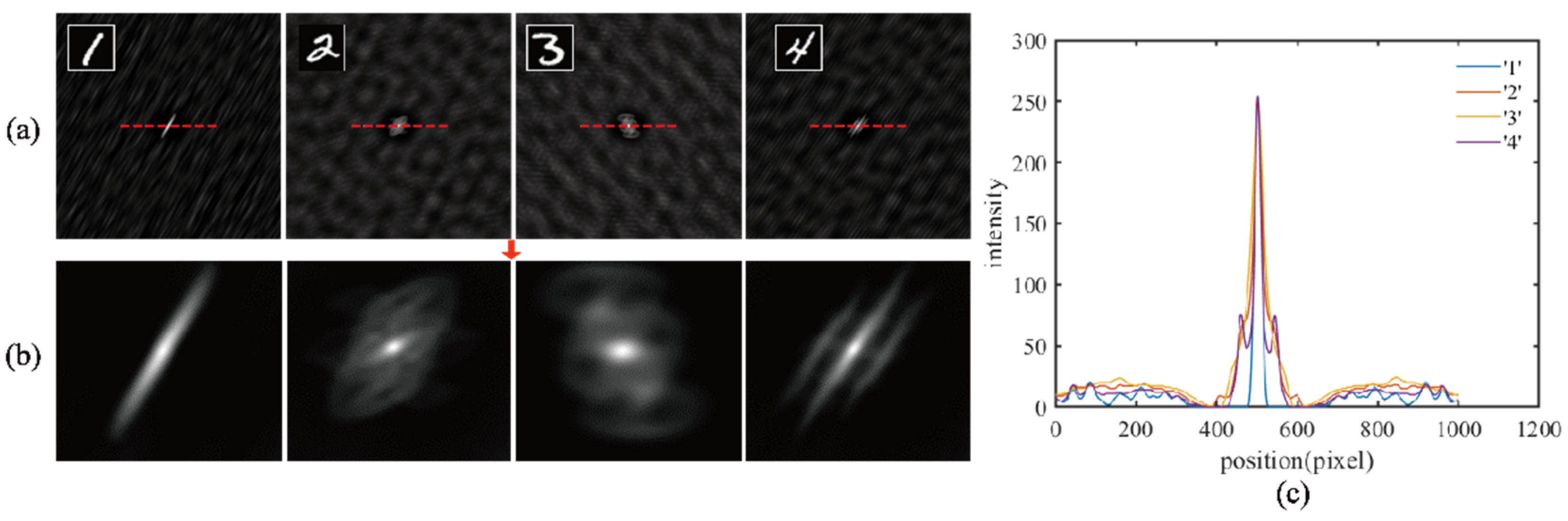
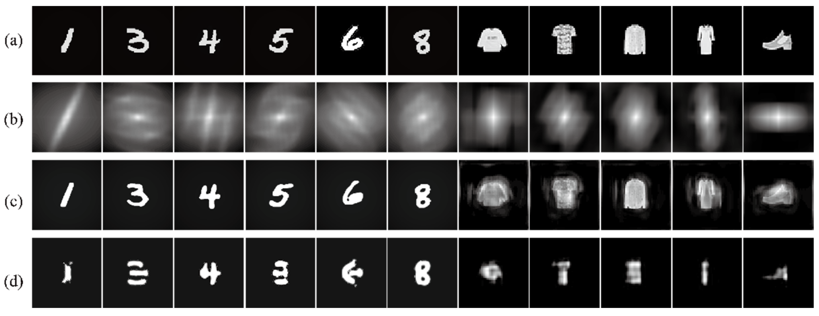
3.4. Experimental Validation

After network training, a comparison was conducted between the images reconstructed by the deep learning method without physics priors and those with priors, respectively. The reconstructed results of some selected testing data are shown in Figure 8. Figure 8a are the ground truths, and Figure 8b are corresponding enlarged views of the autocorrelation functions associated with different speckle images. Figure 8c are the reconstructed results of the proposed method in this paper, and Figure 8d are those without priors. The SSIM is calculated for quantitative assessment. The indicator of the proposed method in this paper is 0.8994, and that without physics priors is 0.8464. Although a few objects can be distinguished without a practical physics prior, such as ‘4’ and ‘8’, it is still hard for the traditional deep learning method to automatically learn the physics relationships between the speckle image and object, implying that the reconstruction is unreliable under the current training dataset and network structure. Additionally, some complex Fashion-MNIST images are tested, as shown in Figure 8 as well. The reconstructed images have a very high fidelity of restoration, but the image details are not satisfactory. In subsequent work, a training set with more samples captured in different CPM cases will make the test results more accurate and reliable.

Then, the proposed method was compared with the traditional reconstruction method, as shown in Figure 9. Figure 9b,c are the reconstruction results of the cross-correlation algorithm and the autocorrelation algorithm. Both reconstruction methods have severe background components, where the average SNRs are 17.10 dB and 10.55 dB, respectively. However, the proposed method can eliminate these effects. The average SNR is up to 92 dB. Thus, the imaging quality is greatly improved. In addition, it can be seen from Figure 9e that the reconstruction result of the proposed method is much closer to the ground truth. Although the cross-section associated with the traditional algorithm can also have the same trend, it is disturbed by the inherent background noise, which leads to a severe error in the reconstructed results.

It has been demonstrated that the reconstructed images of the conventional COACH system are not satisfactory whether reconstructed by cross-correlation or autocorrelation. To reduce the duplication of work, the commonly used cross-correlation method is compared with proposed method on the lateral resolution. Element 4 of Group 6 (G6, E4) in the 1951 USAF resolution target was used to assess the reconstruction strategy. The scale bar is 20 μm in Figure 10. By calculating the contrast modulation (CM), the threshold for visibility is set as 0.4. The imaging resolution of the object reconstructed by the cross-correlation algorithm does not achieve the threshold, where Element 4 corresponds to 33 lp/mm and a bar width of 14.85 μm. On the contrary, the result of the proposed method depicted in Figure 10c demonstrates that Element 4 with a resolution of 90 lp/mm and a bar width of 5.5 μm can be resolved. In addition, the values of SSIM calculated by the two methods are 0.2011 and 0.4373, respectively. The former is influenced by the object points outside the specific axial region, resulting in the out-of-focus image on the camera plane. The latter has a slight distortion for two main reasons. First, the measurement process uses the iris diaphragm to adjust the size of the illuminated area, which shows an octagonal shape. Second, the measured region contains multiple line pairs. Therefore, the structure of the measured object is more complex than the training dataset, which distorts the reconstructed object.

Next, a reflective MEMS sample is adopted for the test, as depicted in Figure 11. The experimental setup in Figure 6 is slightly modified. Figure 11b shows the reconstruction result of the traditional COACH system. Figure 11c depicts the reconstruction result of the proposed method. The corresponding SSIM measures are also provided below. The experimental results indicate that the reconstructed result of the proposed method is closer to the ground truth, and the details are more resolvable.

Finally, to demonstrate the 3D imaging capability of the proposed method, a specific configuration is presented in Figure 12a. Two planar objects O₁ and O₂ were generated from two identical USAF 1951 resolution charts mounted onto channel 1 and channel 2, respectively. First, the location of O₂ in channel 2 was adjusted so that the object plane O₂, modulation plane (SLM plane), and the image plane (camera plane) in channel 2 obeyed a classic 4F imaging relationship. Then, we calculated an apppriate CPM2 associated with the O₂ plane. Similarly, the location of O₁ in channel 1 was adjusted so that the O₁ plane, SLM plane, and camera plane in channel 1 obeyed a classic 4F imaging relationship. Then, we calculated an appropriate CPM1 associated with the O₁ plane. Next, we fixed the plane O₂ and moved the axial position of O₁ in channel 1, with the relative distance Δz = 3, 6, and 10 mm, respectively. CPM2 associated with the O₂ plane was used for reconstruction, and the results are shown in Figure 12c. Similarly, the CPM1 associated with the O₁ plane was used for reconstruction, and the results are provided in Figure 12d. Figure 12c,d demonstrate that the proposed method can reconstruct the 3D object and distinguish two axial planes by using the CPMs of the corresponding planes. Moreover, increasing the relative distance between two planes makes the image reconstruction more difficult. In addition, the reconstruction results are better than those in Figure 10c.

4. Conclusions

This paper introduces a physics-informed deep learning method to improve the imaging quality of the coded aperture correlation holography. Specifically, an explicit framework is established to efficiently eliminate the background noise by combining the prior physics knowledge and deep learning methods. This approach can effectively reduce the training dimension and combine the advantages of model-based methods and the data-driven deep learning methods. The experimental results indicate that the proposed approach can be utilized to remove the background components caused by the cross-correlation algorithm and enhance the quality of the reconstructed image. In the future, more complex scenes and objects will be investigated.

References

1. Dicke, R.H. Scatter-Hole Cameras for X-Rays and Gamma Rays. Astrophys. J. 1968, 153, 101–106. [Google Scholar] [CrossRef]
2. Rosen, J.; Nisan, S.; Gary, B. Theoretical and experimental demonstration of resolution beyond the Rayleigh limit by FINCH fluorescence microscopic imaging. Opt. Express 2011, 19, 26249–26268. [Google Scholar] [CrossRef] [PubMed]
3. Bianco, V.; Mandracchia, B.; Marchesano, V.; Pagliarulo, V.; Olivieri, F.; Coppola, S.; Paturzo, M.; Ferraro, P. Endowing a plain fluidic chip with micro-optics: A holographic microscope slide. Light Sci. Appl. 2017, 6, e17055. [Google Scholar] [CrossRef] [PubMed]
4. Merola, F.; Memmolo, P.; Miccio, L.; Savoia, R.; Ferraro, P. Tomographic flow cytometry by digital holography. Light Sci. Appl. 2016, 6, e16241. [Google Scholar] [CrossRef] [PubMed] [Green Version]
5. Vijayakmar, A.; Kashter, Y.; Kelner, R.; Rosen, J. Coded aperture correlation holography—A new type of incoherent digital holograms. Opt. Express 2016, 24, 2430–2441. [Google Scholar] [CrossRef] [Green Version]
6. Rosen, J.; Anand, V.; Rai, M.R.; Mukherjee, S.; Bulbul, A. Review of 3D imaging by coded aperture correlation holography (COACH). Appl. Sci. 2019, 9, 605. [Google Scholar] [CrossRef] [Green Version]
7. Kelner, R.; Katz, B.; Rosen, J. Optical sectioning using a digital Fresnel incoherent-holography-based confocal imaging system. Optica 2014, 1, 70. [Google Scholar] [CrossRef] [PubMed] [Green Version]
8. Kelner, R.; Rosen, J. Parallel-mode scanning optical sectioning using digital Fresnel holography with three-wave interference phase-shifting. Opt. Express 2016, 24, 2200–2214. [Google Scholar] [CrossRef] [Green Version]
9. Vijayakumar, A.; Rosen, J. Interferenceless coded aperture correlation holography—A new technique for recording incoherent digital holograms without two-wave interference. Opt. Express 2017, 25, 13883–13896. [Google Scholar] [CrossRef] [PubMed] [Green Version]
10. Hai, N.; Rosen, J. Interferenceless and motionless method for recording digital holograms of coherently illuminated 3D objects by coded aperture correlation holography system. Opt. Express 2019, 27, 24324–24339. [Google Scholar] [CrossRef]
11. Hai, N.; Rosen, J. Coded aperture correlation holographic microscope for single-shot quantitative phase and amplitude imaging with extended field of view. Opt. Express 2020, 28, 27372–27386. [Google Scholar] [CrossRef]
12. Hai, N.; Rosen, J. Doubling the acquisition rate by spatial multiplexing of holograms in coherent sparse coded aperture correlation holography. Opt. Lett. 2020, 45, 3439–3442. [Google Scholar] [CrossRef]
13. Rai, M.R.; Rosen, J. Noise suppression by controlling the sparsity of the point spread function in interferenceless coded aperture correlation holography (I-COACH). Opt. Express 2019, 27, 24311–24323. [Google Scholar] [CrossRef]
14. Vijayakmar, A.; Rosen, J.; Ratnam, M. Single camera shot interferenceless coded aperture correlation holography. Opt. Lett. 2017, 42, 3992–3995. [Google Scholar]
15. Rai, M.R.; Vijayakumar, A.; Joseph, R. Non-linear adaptive three-dimensional imaging with interferenceless coded aperture correlation holography (I-COACH). Opt. Express 2018, 26, 18143–18154. [Google Scholar] [CrossRef]
16. Wan, Y.; Liu, C.; Ma, T.; Qin, Y.; Lv, S. Fast and Noise-suppressed Incoherent Coded Aperture Correlation Holographic Imaging. Opt. Express 2021, 29, 8064–8075. [Google Scholar] [CrossRef] [PubMed]
17. Nishizaki, Y.; Valdivia, M.; Horisaki, R.; Kitaguchi, K.; Saito, M.; Tanida, J.; Vera, E. Deep learning wavefront sensing. Opt. Express 2019, 27, 240–251. [Google Scholar] [CrossRef] [PubMed]
18. Nehme, E.; Weiss, L.E.; Michaeli, T.; Shechtman, Y. Deep-STORM: Super-resolution single-molecule microscopy by deep learning. Optica 2018, 5, 458–464. [Google Scholar] [CrossRef] [Green Version]
19. Wang, W.B.; Wu, B.W.; Zhang, B.Y.; Ma, J.; Tan, J.B. Deep learning enables confocal laser-scanning microscopy with enhanced resolution. Opt. Lett. 2021, 46, 4932–4935. [Google Scholar] [CrossRef] [PubMed]
20. Choi, G.; Ryu, D.H.; Jo, Y.J.; Kim, Y.S.; Park, Y.K. Cycle-consistent deep learning approach to coherent noise reduction in optical diffraction tomography. Opt. Express 2019, 27, 4927–4943. [Google Scholar] [CrossRef] [Green Version]
21. Rivenson, Y.; Zhang, Y.; Gunaydin, H.; Da, T.; Ozcan, A. Phase recovery and holographic image reconstruction using deep learning in neural networks. Light Sci. Appl. 2017, 7, 192–200. [Google Scholar] [CrossRef] [PubMed]
22. Wang, H.; Lyu, M.; Situ, G. eHoloNet: A learning-based end-to-end approach for in-line digital holographic reconstruction. Opt. Express 2018, 26, 22603–22614. [Google Scholar] [CrossRef] [PubMed]
23. Wu, Y.; Yair, R.; Zhang, Y.; Wei, Z.; Harun, G.; Xing, L.; Aydogan, O. Extended depth-of-field in holographic imaging using deep-learning-based autofocusing and phase recovery. Optica 2018, 5, 704–710. [Google Scholar] [CrossRef] [Green Version]
24. Liu, T.; Wei, Z.; Rivenson, Y.; Haan, K.D.; Ozcan, A. Deep learning-based color holographic microscopy. J. Biophotonics 2019, 12, e201900107. [Google Scholar] [CrossRef] [Green Version]
25. Wang, F.; Bian, Y.; Wang, H.; Meng, L.; Pedrini, G.; Osten, W.; Barbastathis, G.; Situ, G. Phase imaging with an untrained neural network. Light Sci. Appl. 2020, 9, 499–505. [Google Scholar] [CrossRef] [PubMed]
26. Fang, L.; David, C.; Chong, W.; Guymer, R.H.; Li, S.; Sina, F. Automatic segmentation of nine retinal layer boundaries in OCT images of non-exudative AMD patients using deep learning and graph search. Biomed. Opt. Express 2017, 8, 2732–2744. [Google Scholar] [CrossRef] [PubMed] [Green Version]
27. Nguyen, T.; Bui, V.; Nehmetallah, G. Computational optical tomography using 3-D deep convolutional neural networks. Opt. Eng. 2018, 57, 043111. [Google Scholar]
28. Shuai, L.; Mo, D.; Justin, L.; Ayan, S.; George, B. Imaging through glass diffusers using densely connected convolutional networks. Optica 2018, 5, 803–813. [Google Scholar]
29. Yang, M.; Liu, Z.H.; Cheng, Z.D.; Xu, J.S.; Li, C.F.; Guo, G.C. Deep Hybrid Scattering Image Learning. J. Phys. D Appl. Phys. 2018, 52, 115105. [Google Scholar] [CrossRef] [Green Version]
30. Ulyanov, D.; Vedaldi, A.; Lempitsky, V. Deep Image Prior. In Proceedings of the 2018 IEEE/CVF Conference on Computer Vision and Pattern Recognition, Salt Lake City, UT, USA, 18–23 June 2018. [Google Scholar]
31. Bertolotti, J.; Putten, E.; Blum, C.; Lagendijk, A.; Mosk, A.P. Non-invasive imaging through opaque scattering layers. Nature 2012, 491, 232–234. [Google Scholar] [CrossRef]
32. Katz, O.; Heidmann, P.; Fink, M.; Gigan, S. Non-invasive single-shot imaging through scattering layers and around corners via speckle correlations. Nat. Photonics 2014, 8, 784–790. [Google Scholar] [CrossRef] [Green Version]
33. Porat, A.; Andresen, E.R.; Rigneault, H.; Oron, D. Widefield lensless imaging through a fiber bundle via speckle correlations. Opt. Express 2016, 24, 16835–16855. [Google Scholar] [CrossRef] [PubMed]
34. Cohen, L. Generalization of the Wiener-Khinchin theorem. IEEE Signal Process. Lett. 1998, 5, 292–294. [Google Scholar] [CrossRef]
35. Fienup, J.R. Phase retrieval algorithms: A comparison. Appl. Opt. 1982, 21, 2758–2769. [Google Scholar] [CrossRef] [Green Version]
36. Miao, J. Extending the methodology of X-ray crystallography to allow imaging of micorometre-sized non-crystaalin speciments. Nature 1999, 400, 342–344. [Google Scholar] [CrossRef]
37. Kuschmierz, R.; Scharf, E.; Ortegón-González, D.; Glosemeyer, T.; Czarske, J.W. Ultra-thin 3D lensless fiber endoscopy using diffractive optical elements and deep neural networks. Light Adv. Manuf. 2021, 2, 415–424. [Google Scholar] [CrossRef]
38. Pohle, D.; Rothe, S.; Koukourakis, N.; Czarske, J.J.O.L. Surveillance of few-mode fiber-communication channels with a single hidden layer neural network. Opt. Lett. 2022, 47, 1275–1278. [Google Scholar] [CrossRef]
39. Li, X.; Li, R.; Zhao, Y.; Zhao, J. An improved model training method for residual convolutional neural networks in deep learning. Multimed. Tools Appl. 2021, 80, 6811–6821. [Google Scholar] [CrossRef]
40. Zhu, S.; Guo, E.; Gu, J.; Bai, L.; Han, J. Imaging through unknown scattering media based on physics-informed learning. Photonics Res. 2021, 9, B210–B219. [Google Scholar] [CrossRef]
41. Zhou, Y.; Zhang, M.; Zhu, J.; Zheng, R.; Wu, Q. A Randomized Block-Coordinate Adam online learning optimization algorithm. Neural Comput. Appl. 2020, 32, 12671–12684. [Google Scholar] [CrossRef]
42. Kayed, M.; Anter, A.; Mohamed, H. Classification of Garments from Fashion MNIST Dataset Using CNN LeNet-5 Architecture. In Proceedings of the 2020 International Conference on Innovative Trends in Communication and Computer Engineering (ITCE), Aswan, Egypt, 8–9 February 2020. [Google Scholar]
Figure 1. Optical configuration of I-COACH in coherent imaging system.
Photonics 09 00967 g001
Figure 2. Analysis of the similarity of speckle images modulated by different CPMs. (a) The cross-correlation with CPM4; (b) Profiles of the red dashed lines in (a).
Photonics 09 00967 g002
Figure 3. Autocorrelation analysis of the same object corresponding to different CPMs. (a) The autocorrelation of object; (b) The autocorrelation of speckle; (c) Profiles of the red dashed lines in (a,b).
Photonics 09 00967 g003
Figure 4. Autocorrelation analysis of different objects associated with the same CPM. (a) The autocorrelations of objects; (b) Enlarged partial views of (a); (c) Profiles of the red dashed lines of (a).
Photonics 09 00967 g004
Figure 5. Schematic of the physics-informed deep learning method.
Photonics 09 00967 g005
Figure 6. Optical configuration.
Photonics 09 00967 g006
Figure 7. HOBJ and reconstructed images for different HPSF. (ac) are associated with 8, 15, and 20 dots, respectively; (df) are the corresponding reconstructed images.
Photonics 09 00967 g007
Figure 8. Comparison of the reconstructed results without or with physics priors. (a) Ground truth; (b) Enlarged partial views of the autocorrelation image of speckle; (c) Results using the proposed strategy; (d) Results without priors.
Photonics 09 00967 g008
Figure 9. Comparison between the proposed method and the correlation algorithm. (a) Ground truth; (b) Result of the cross-correlation algorithm; (c) Result of the autocorrelation algorithm; (d) Result of the proposed strategy; (e) Profiles of the dashed red lines in (ad).
Photonics 09 00967 g009
Figure 10. Experimental results of 1951 USAF target. (a) Ground truth; (b) Results of the cross-correlation algorithm; (c) Results of the proposed strategy; (d) Un-cropped object by the proposed strategy; (e) Profiles of the red dashed lines in (ac).
Photonics 09 00967 g010
Figure 11. Experimental results of a MEMS element. (a) Ground truth; (b) Result of the cross-correlation algorithm (SSIM: 0.2651); (c) Result of the proposed strategy (SSIM: 0.5793); (d) Intensity values of the red dashed lines in (ac).
Photonics 09 00967 g011
Figure 12. Demonstration of the 3D imaging reconstruction process of the proposed method by the separation between two planes Δz. (a) Optical system configuration (BE: beam expander. P: polarizer. L1, L2: lens. SLM: spatial light modulation); (b) Uncropped object by the proposed strategy; (c) Reconstruction using CPM2 of O2 plane; (d) Reconstruction using CPM1 of O1 plane.
Photonics 09 00967 g012