Article

Measurement of the Attenuation Coefficient in Fresh Water Using the Adjacent Frame Difference Method

Institute of Marine Optoelectronic Equipment, Harbin Institute of Technology at Weihai, Weihai 264209, China
*
Authors to whom correspondence should be addressed.
Photonics 2022, 9(10), 713; https://doi.org/10.3390/photonics9100713
Submission received: 30 July 2022 / Revised: 15 September 2022 / Accepted: 24 September 2022 / Published: 30 September 2022
(This article belongs to the Section Optical Interaction Science)

Abstract

:
The attenuation coefficient of a water body is one of the important factors for describing its features. However, its remote measurement in real time is still a challenge. In this paper, we demonstrated a novel method to realize real-time remote measurements of the attenuation coefficient of fresh water using flash imaging lidar based on the adjacent frame difference (AFD) method and a water body backscattering model. In general, we firstly investigated the relationship between the backscattering intensity and the attenuation coefficient based on the backscattering model of the water body. Then, the backscattering intensity at the front and back edges of the range-gate obtained by the AFD method was brought into this relationship to obtain the attenuation coefficient. Experiments on the measurements of the average attenuation coefficient of the 532 nm laser in fresh water at 3–8 m were further carried out using our self-developed flash lidar with the AFD method. The acquired water attenuation coefficients were 0.1334 ± 0.02 and 0.1382 ± 0.03 with a delay step time of 1 ns and 2 ns in the AFD method, respectively. We compared these values to the one achieved following the conventional Beer–Lambert law ( 0.1330 ± 0.02 ), and they matched well with each other. These results fully illustrated the feasibility and reliability of the proposed method for measuring the attenuation coefficient of water bodies.

1. Introduction

Water attenuation coefficient is one of the important factors to quantify the transmission rate of a water body [1,2,3], which is also used to evaluate the efficiency of light transportation in water, underwater visibility conditions and serves as an indicator of contaminations [4,5,6]. In addition, the water attenuation coefficient plays a key role in underwater measurements based on the lidar system. Therefore, the real-time measurement of the attenuation of the water body is of great significance for the future development of underwater engineering technology and basic physical experiments.
In recent years, much attention has been paid to the measurement of the water attenuation coefficient. Different methods have been developed, such as the Beer–Lambert law [7,8,9,10], Raman scattering [11,12], through the stimulated Brillouin scattering [13,14,15] and the Weibull shape parameters of the Lidar waveforms [16], as well as measuring its apparent optical properties [15,17,18,19,20,21,22]. The Beer–Lambert law is one of the direct and accurate measurements within a certain range. However, this method needs to sample the water body or constantly change the position of the power meter, which makes it difficult to realize in the real-time remote measurement of the attenuation coefficient of the water body. Other methods either have complex optical paths or do not enable real-time remote sensing measurements.
In this work, by combining the backscattering model of a water body and the adjacent frame difference (AFD) method [23], we demonstrate a novel method to remotely measure the attenuation coefficient of water in real time. The relationship between the backscattering intensity of the water and the water attenuation coefficient is derived from the backscattering model of the water body [24]. Based on this relationship and the backscattered intensity in the water measured by the AFD method, the water attenuation coefficient can be calculated. Experimental results and a theoretical analysis fully illustrate the feasibility and reliability of the AFD method on measuring the attenuation coefficient of water body.

2. Methods

We established a backscattering model in the water to build up the relationship between the water attenuation coefficient of the water body and the backscattering intensity value obtained by AFD method in real time.

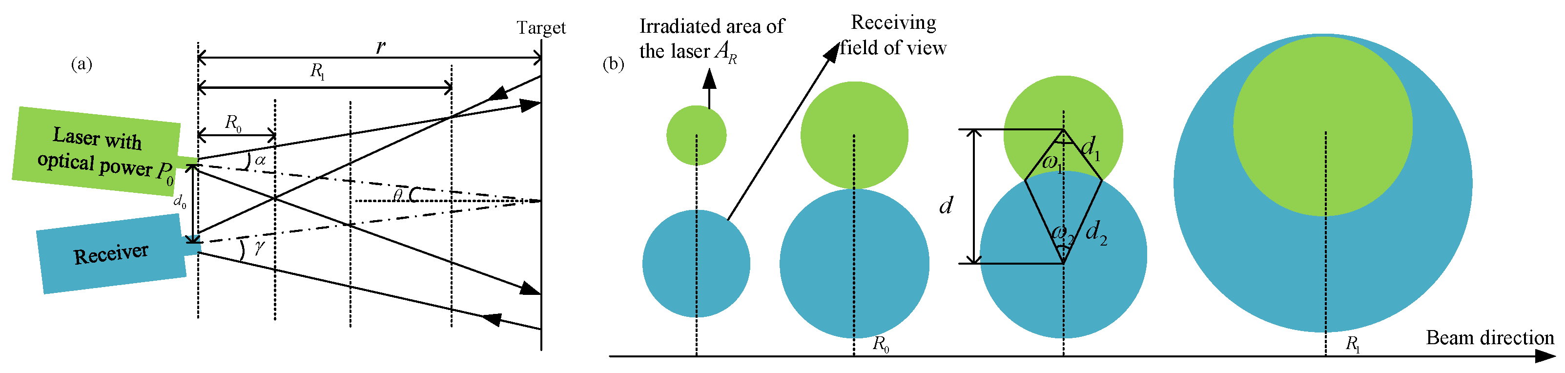
2.1. Backscattering Model in the Water

Essentially, both the light backscattering of a water body and the echo light of the target underwater represent the reflection signals from different objects in the water. Therefore, according to the principle of underwater light transmission and reflection provided by the lidar equation, a computational model of backscattered light from the water body can be established [25].
The schematic diagram of the backscattering model of the water body is shown in Figure 1a. In this figure, α is the half divergence angle of the laser, γ is the half field of view of the receiver, P 0 is the output laser optical power, θ is half of the angle between the transmitting center axis and the receiving center axis, r is the distance of the target from the Lidar system, d 0 is the distance of the transmitting center and receiving center, A ( r ) is the irradiated area of the laser at distance of r and C is the attenuation coefficient of water. The total backscattered luminous flux from the water body can be obtained as [26]:
P = A R cos θ P 0 U e 2 C r cos   θ A ( r ) r 2 d A d r ,
where U is the backward scattering coefficient and A R is the effective receiving area.
As shown in Figure 1b, the geometry sizes of the laser spot and received field-of-view interface vary with the distances between the laser source and target, which results in changes on their overlap area. In order to analyze the backscattering with different overlap area between the laser spot and the received field of view, an overlap factor F was introduced, which was defined as the ratio of the laser spot area captured in the received field of view to the total laser irradiation area. It was expressed as [27]:
F = 1 A ( r ) d A ,
In Figure 1b, the angles corresponding to the overlapping area sections on the cross sections of the laser spot and received field of view are defined as ω 1 and ω 2 , respectively; d 1 and d 2 are the radius of the laser spot and the receiving field of view, respectively; and d is the distance between the centers of the laser spot and the receiving field of view. The radii of the transmitting optical system and the receiving optical system are r L and r R , respectively. Then, the detailed expression for the overlapping area at different positions can be calculated from the trigonometric relationship:
F = 0 F = 1 F = d 1 2 ( ω 1 sin   ω 1 ) + d 2 2 ( ω 2 sin   ω 2 ) 2 π d 1 2 ( r R 0 ) ( r R 0 ) ( R 0 r R 1 )
where R 0 is the distance corresponding to the laser spot and the received field of view when they are externally tangent to each other; R 1 is the distance corresponding to the laser spot and received field of view when they are internally tangent to each other; and r is the detection distance. The introduction of F reduces the dimension of the integral of Equation (1) and turns the double integral into an ordinary integral to simplify calculations. According to Equations (1) and (2), the total backscattering flux of the water body can be further expressed as:
P = A R cos θ P 0 U F e 2 C r cos   θ r 2 d r
Differentiating Equation (4) with respect to distance r yields:
d P b d r = A R cos θ P 0 U F e 2 C r cos   θ r 2
Then, the relationship between the backscattering intensity and the attenuation coefficient of the water body can be obtained:
C = 1 2 r cos θ ln d P b d r r 2 A R cos θ P 0 U F
It can be found that in Equation (6), only r and d P b d r are unknown value. Therefore, the attenuation coefficient of the water body can be calculated as long as the d P b d r and corresponding distance r have been measured. Our AFD method is a novel approach to acquire the backscattering intensity of the water body and corresponding distance information in real time. The basic principle of the AFD method is introduced in the next subsection.

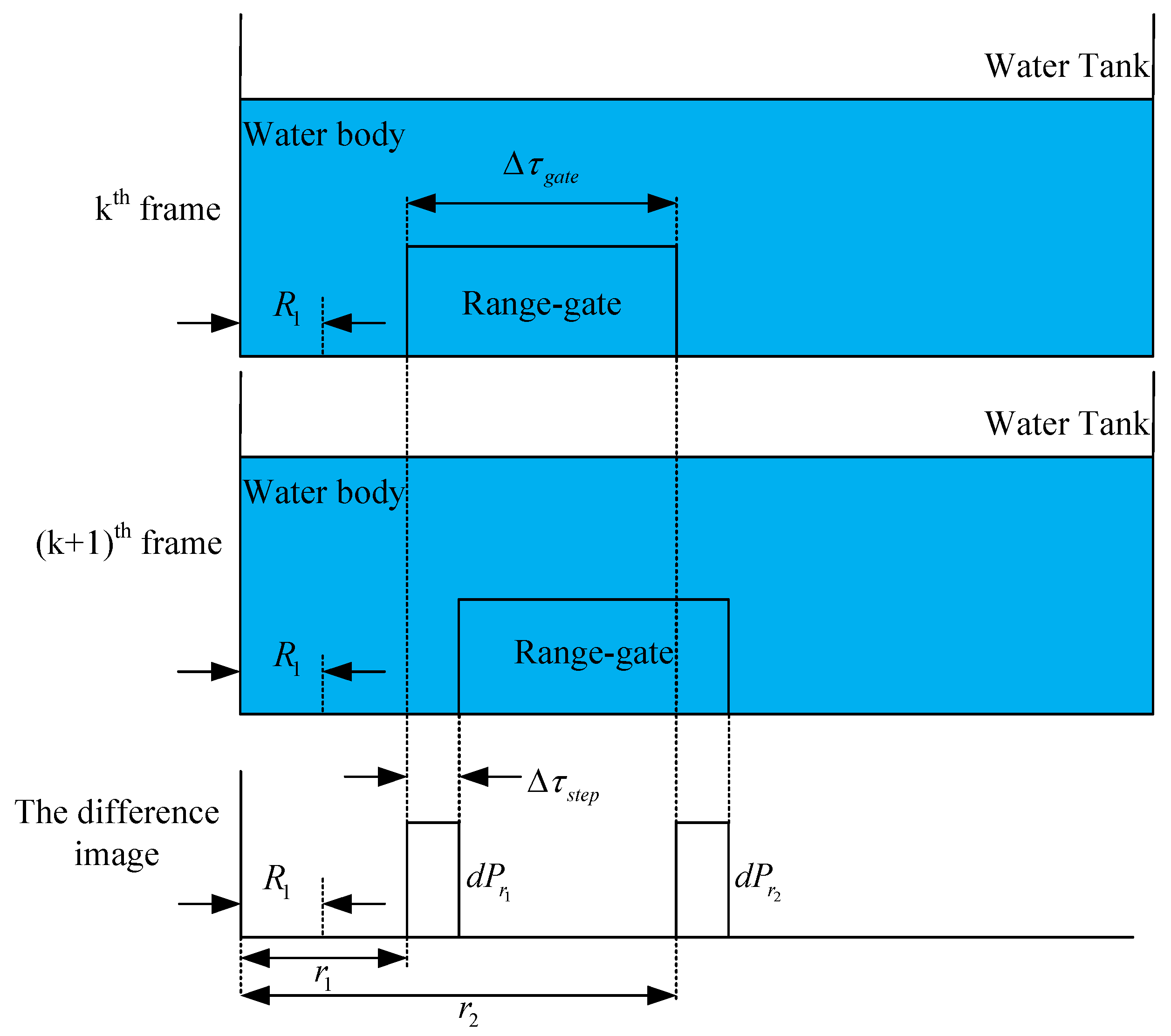
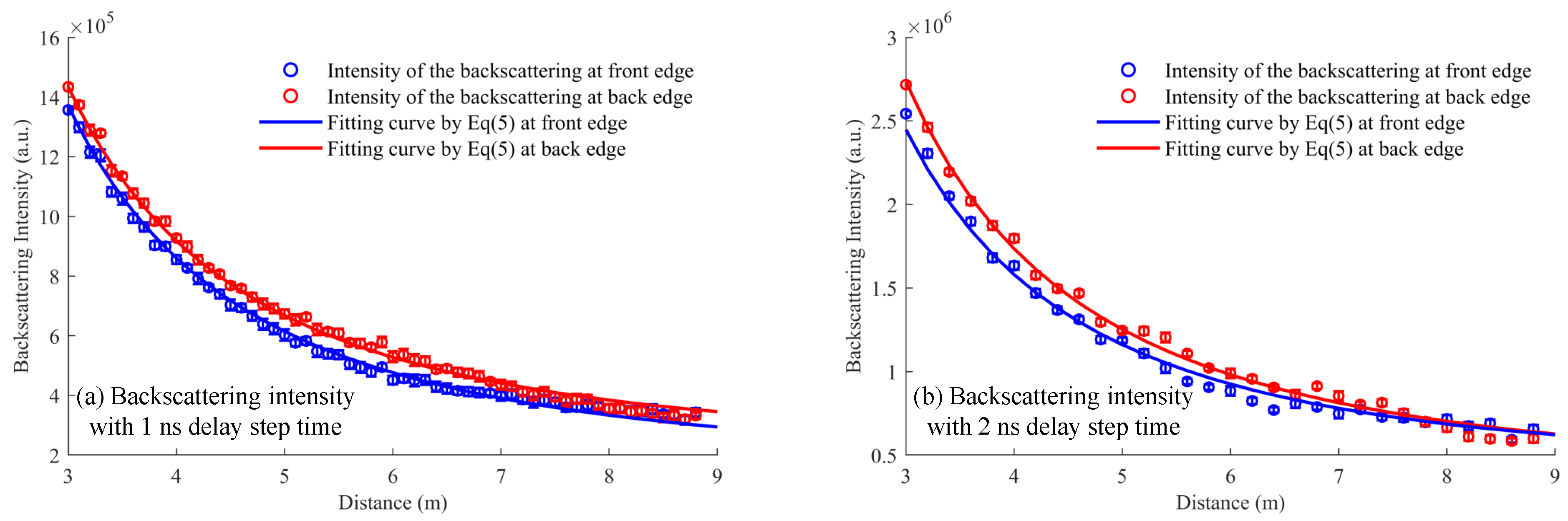
2.2. Obtaining the Backscattering Intensity by the AFD Method
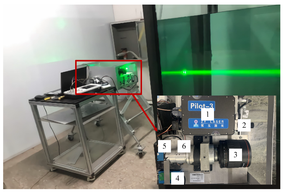
The AFD method is a new three-dimensional (3D) reconstruction algorithm based on the range-gated method [23]. In this method, the distance information of the target at the front and back edges of the range-gate are obtained by thresholding the intensity difference between two adjacent frames achieved by the intensified-charge-coupled device (ICCD). According to the characteristics of the AFD method, it is known that the AFD method can obtain the backscattering intensity corresponding to the front and back edges of the range-gate in real time.
Figure 2 presents the principal diagram of the AFD method to measure the backscattering intensity in the water. As is shown, Δ τ g a t e is the width of the range-gate and Δ τ s t e p is the delay step size of the flash lidar system. If the distance is larger than R 1 ( F = 1 ), the intensity image acquired by the ICCD is the backscattering intensity of the water body. The corresponding intensity difference image Δ I k can be acquired by the backscattering intensity images of k t h frame and k + 1 t h frame obtained by the lidar. Therefore, the back edge of the range-gate part in their difference image Δ I ( i , j ) k is the backscattering intensity at r 1 and the front edge of the range-gate part in their difference image Δ I ( m , n ) k is the backscattering intensity at r 2 . Assuming the backscattering intensities at the back and front edges of the range-gate are d P r 1 and d P r 2 :
d P r 1 = Δ I ( i , j ) k , d P r 2 = Δ I ( m , n ) k
According to Equation (6), Equation (7) and d P r 1 d P r 2 , we can get:
C = ln Δ I ( i , j ) k Δ I ( m , n ) k ln r 2 2 r 1 2 2 ( r 2 r 1 ) cos θ
where r 1 = v ( Δ τ + k Δ τ s t e p ) , r 2 = v [ Δ τ + ( k + 1 ) Δ τ s t e p ] , v is the light speed in the water and Δ τ is the initial delay of the lidar system.

3. Experiments

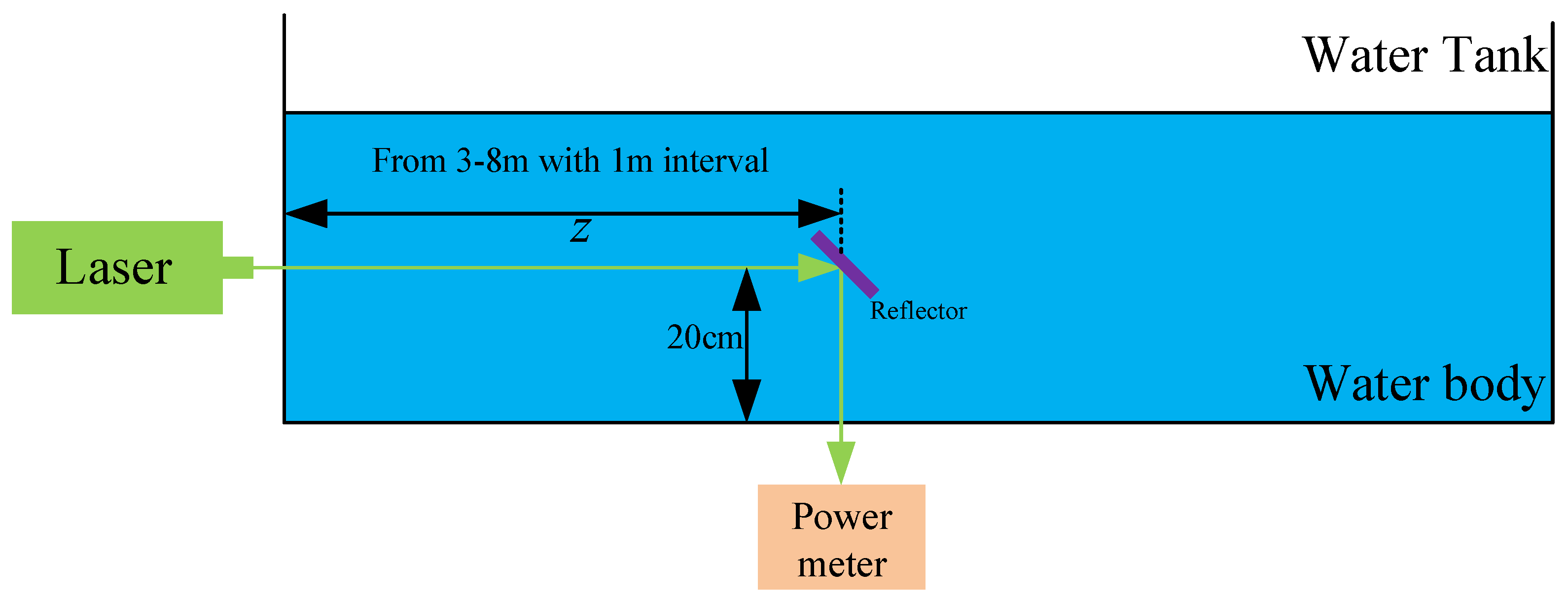
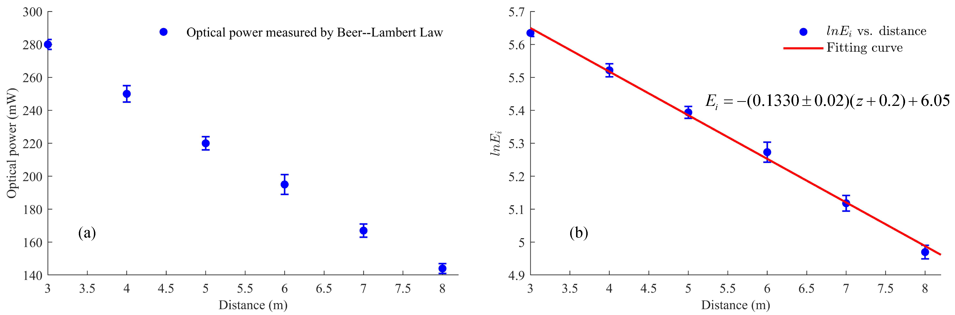
3.1. Measurement of the Water Attenuation Coefficient by the Beer–Lambert Law

In order to verify the reliability of the AFD method, we used the Beer–Lambert law method as a reference. The Beer–Lambert law represents the relationship between the attenuation of light and the property of medium. It asserts that light intensity diminishes exponentially as a function of the traveling depth in the medium.
The schematic diagram of this experiment is shown in Figure 3. As is shown, the incident laser beam vertically propagated through the glass wall of the water tank and water body. Then, it was reflected by a reflector at different propagating distances and measured by a laser power meter outside the water tank. The measured propagating distances were from 3 to 8 m with 1 m interval and each point was measured five times. The laser system in this experiment was the same as that used in the AFD method. By assuming that the amount of attenuation caused by other factors, such as pool glass and reflectors, was η , the received optical power at different distances could be expressed as:
E i = η E 0 e C ( z + 0.2 )
where E 0 is the initial optical power of light source, C is the attenuation coefficient of the water body and z is the measuring distance between the reflector and light source. E i is the optical power received at different distances. Taking the logarithm of Equation (9), we can get:
ln ( E i ) = C ( z + 0.2 ) + ln η E 0
The average measured optical power of the laser beam at 3–8 m propagating distances in the water body with 1 m interval are shown in Figure 4a. Based on these experimental data and Equation (10), the fitting curve is shown in Figure 4b. The blue dots represent the l n ( E i ) value obtained from the measurements at different propagating distances and the red curve represents the equation of the line obtained using a linear fit, which was ln ( E i ) = ( 0.1330 ± 0.02 ) ( z + 0.2 ) + 6.05 with a coefficient of determination of 0.9945. According to the Equation (10), the attenuation coefficient of the water body based on the Beer–Lambert law was calculated as 0.1330 ± 0.02 .

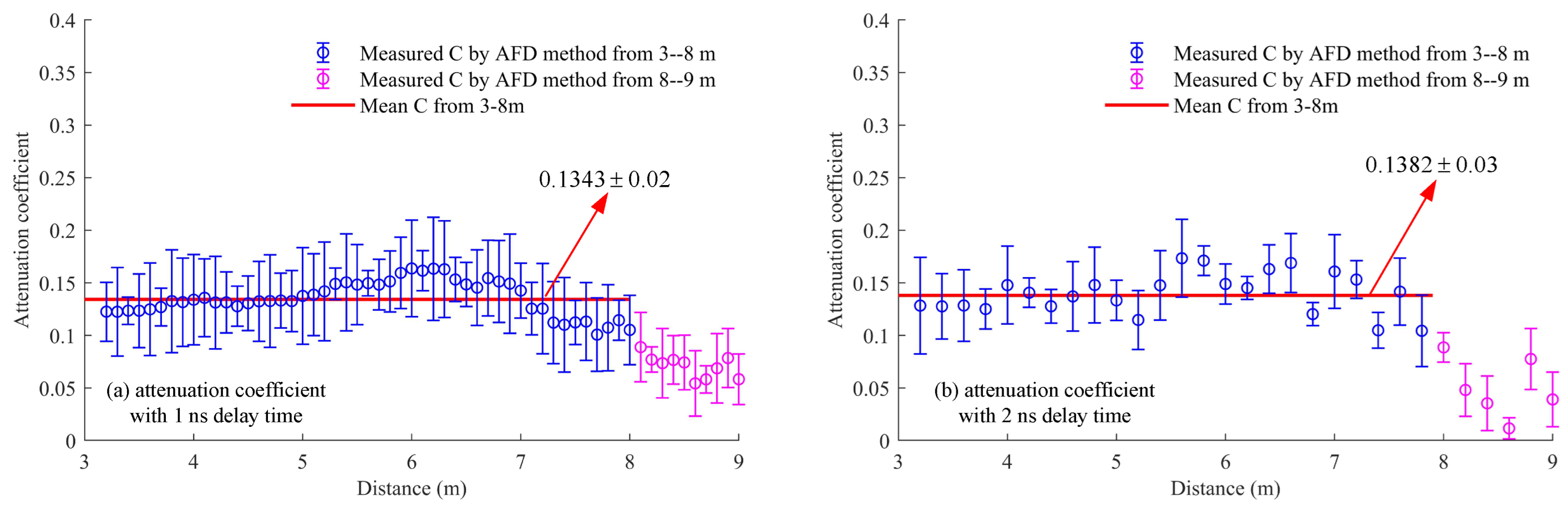
3.2. Experimental Measurement of Water Attenuation Coefficient by AFD Method

Based on the model established in the last two subsections, we carried out the experimental measurements on the attenuation coefficient of the water body in the glass water tank using a self-developed flash lidar system. An image of the experimental setup is shown in Figure 5. A 30 m long and 2 m wide water tank was used. The height of the water body in the tank was about 1.2 m. The emission wavelength of the used flash laser lidar system was 532 nm. The pulse width and pulse repeat frequency were 5 ns and 1 kHz, respectively. The diameter of the laser spot was 1 mm. The laser divergence angle was adjusted by a collimation system. A Cassegrain lens was used to receive the backscattering signal, an optical filter with a central wavelength of 532 nm and a bandwidth of 3 nm was used to reduce the background noise. The resolution of the CCD was 1292 × 964 . Furthermore, in order to ensure F = 1 , according to the geometric relationship shown in Figure 1, the experimental setup was adjusted following the parameters listed in Table 1. The distance between laser and the receiving system d 0 was 20 cm, the half-divergence angle of the laser α was 2.86 , the half field of view of the receiving system was 8.36 and the angle between the center axis of the laser and the center axis of the receiving system was 0. R 0 was 1 m, R 1 was 1.5 m and the range-gate width was 20 ns.
Figure 6a,b demonstrate the averaged backscattered intensity values from five measurements of the water body at the propagating distances from 3 m to 9 m using the AFD method with delay step times of 1 ns and 2 ns, respectively. In both figures, the red and blue spots represent the backscattered intensities of the water body at the back and front edges of the range-gate. As is shown, the backscattering intensities at the back edge of the range-gate were higher than the ones at the front edge of the range-gate, which was due to the closer distance between the back edge of the range-gate and the flash lidar system. It could be also found that, as the distance increased, the absolute backscattering intensity values, whether measured through the back or front edges of the range-gate, gradually decreased. The intensity differences between the front and back edge backscattering decreased when the distance increased. That is because the right side of Equation (5) is a decreasing function and its second derivative is a positive value when r > 0 . The red and blue curves represent the fitting curve of the measurement value by Equation (5) at the back and front edges of the range-gate. Their coefficients of determination were all greater than 0.98 . Meanwhile, both phenomena showed a great agreement with the trends predicted by Equation (5), which indicated the accuracy of the water backscattering model.
Based on the measured backscattering intensity of the water body at the front and back edge of the range-gate from the AFD method and according to the Equation (8), the attenuation coefficients of the water body at a 3–9 m propagating distance is shown in Figure 7 with 1 ns (part (a)) and 2 ns (part (b)) delay step times, respectively. Due to the relatively lower signal-to-noise ratio (SNR) of the ICCD when measuring the backscattering intensity at 8–9 m in the water, the measured backscattering intensity of the water body at the back and front edges of the range-gate were mixed together (as shown in Figure 6), leading to the calculated attenuation coefficient at 8–9 m in the water not being very accurate (as shown in the pink circle in Figure 7). Therefore, the measurements at 8–9 m were excluded when calculating the average attenuation coefficient. The average attenuation coefficients of the water body at 3–8 m with different delay step times were calculated and are represented by the red curve in Figure 7, corresponding to 0.1343 ± 0.02 and 0.1381 ± 0.03 with 1 ns and 2 ns delay step times. Here, we would like to emphasize that the water attenuation coefficient achieved under the shorter delay step time should be more accurate, because the parameter of d P b d r is a differential form, and according to Figure 2, the smaller the delay step time, the higher the accuracy.

4. Discussion

Compared with the water attenuation coefficient achieved by the Beer–Lambert law ( 0.1330 ± 0.02 ), the relative errors measured by our AFD method at 1 ns and 2 ns delay steps were 0.98 % and 3.91 % , respectively. The relative error of the values obtained at 1 ns was smaller than that obtained at 2 ns, which agreed well with our analysis results in Section 3.2.
In addition, the water attenuation coefficient obtained by the fitting curves in Figure 6a,b were 0.1287 and 0.1232 , respectively. The relative errors achieved by this fitting method were 3.23 % and 7.37 % under the delay step times of 1 ns and 2 ns, which were larger than the relative error of the AFD method. For example, when the delay step was 2 ns, the relative error in the AFD method was only 3.91 % , even though the number of points measured was only half of that at 1 ns. Therefore, the AFD method can overcome the disadvantage of fitting methods that need to measure enough points to ensure their accuracy.
The relative error between the attenuation coefficients measured at different propagating distances by the AFD method with a delay step time of 1 ns and the Beer–Lambert law was further compared. As shown in Table 2, the relative errors for the Beer–Lambert law were 6.82 % , 0.82 % , 5.26 % , 3.78 % and 9.38 % and the relative errors for the AFD method were 4.76 % , 2.89 % , 2.59 % , 4.82 % and 0.11 % in the ranges of 3–4 m, 3–5 m, 3–6 m, 3–7 m and 3–8 m. Their average relative errors were 5.21 % and 3.04 % . The standard deviation of the water attenuation coefficient in different distance ranges measured by the AFD method was 0.0052, which was smaller than the one from the Beer–Lambert law as 0.0083. Compared with the one for the Beer–Lambert law, it can be clearly found that the absolute errors for the AFD method did not change abruptly as the range changed. Therefore, as the measurement range increased, the AFD method was more stable than the Beer–Lambert law. These results fully demonstrated that the attenuation coefficient of water body measured by the AFD method in real time was feasible and credible.

5. Conclusions

In this paper, a method for real-time remote measurement of the water attenuation coefficient was proposed. We firstly derived the relationship between the backscattering intensity and the attenuation coefficient of the water body by establishing a backscattering model of the water body. Based on this relationship and the AFD method, the attenuation coefficient of the water body could be further calculated in real time. In order to verify the feasibility of this method, a self-developed flash lidar system was used to conduct a measurement study of a freshwater body at the distance range of 3–8 m. The attenuation coefficient of the water body was measured as 0.1343 ± 0.02 and 0.1382 ± 0.03 under 1 ns and 2 ns delay step times for the AFD method. By comparing the Beer–Lambert law and the AFD method at different distance ranges, the experimental results and theoretical analysis fully verified the feasibility and reliability of the AFD method to measure the attenuation coefficient of water bodies. The attenuation coefficient of water measured by the AFD method is applicable to all waters that satisfy the backscattering model. However, our method is not applicable to very turbid water bodies due to the effects of multiple scattering. In our future research, a high SNR camera can be used to improve the measurement range of the AFD method.

Author Contributions

Conceptualization, G.Y. and Z.T.; data curation, G.Y. and Q.L.; formal analysis, G.Y. and Q.L.; funding acquisition, Z.T.; investigation, Z.T.; methodology, G.Y. and Q.L.; project administration, Z.T.; resources, Z.T.; software, G.Y., Z.T., Z.B. and Z.C.; supervision, Z.T.; validation, G.Y., Z.B., Z.C. and Q.L.; writing—original draft, G.Y., Z.T., F.S. and Q.L.; writing—review and editing, G.Y., Z.T., F.S. and Q.L. All authors have read and agreed to the published version of the manuscript.

Funding

This work was supported by the China National Key R&D Program under Grant 2020YFE0201500 and the Excellent Youth Science Foundation of Shandong Province (Overseas) under Grant 2022HWYQ-073.

Institutional Review Board Statement

Not applicable.

Informed Consent Statement

Not applicable.

Data Availability Statement

Not applicable.

Conflicts of Interest

The authors declare no conflict of interest.

Abbreviations

The following abbreviations are used in this manuscript:
AFDAdjacent frame difference
3DThree-dimensional
ICCDIntensified-charge-coupled device
SNRSignal-to-noise ratio

References

  1. Babin, M.; Roesler, C.S.; Cullen, J.J. Real-Time Coastal Observing Systems for Marine Ecosystem Dynamics and Harmful Algal Blooms: Theory, Instrumentation and Modelling; Unesco: London, UK, 2008. [Google Scholar]
  2. Ingles, J.; Louw, T.M.; Booysen, M. Water quality assessment using a portable UV optical absorbance nitrate sensor with a scintillator and smartphone camera. Water SA 2021, 47, 135–140. [Google Scholar]
  3. Min, R.; Liu, Z.; Pereira, L.; Yang, C.; Sui, Q.; Marques, C. Optical fiber sensing for marine environment and marine structural health monitoring: A review. Opt. Laser Technol. 2021, 140, 107082. [Google Scholar] [CrossRef]
  4. Gasowski, R.A.; Pawlak, B. Light attenuation in waters of the Oder River and Pomeranian Bay. In Proceedings of the 13th Polish-Czech-Slovak Conference on Wave and Quantum Aspects of Contemporary Optics. International Society for Optics and Photonics, Krzyżowa, Poland, 9–13 September 2002; Volume 5259, pp. 372–378. [Google Scholar]
  5. Sullivan, J.M.; Donaghay, P.L.; Rines, J.E. Coastal thin layer dynamics: Consequences to biology and optics. Cont. Shelf Res. 2010, 30, 50–65. [Google Scholar] [CrossRef]
  6. Chang, N.; Luo, L.; Wang, X.C.; Song, J.; Han, J.; Ao, D. A novel index for assessing the water quality of urban landscape lakes based on water transparency. Sci. Total Environ. 2020, 735, 139351. [Google Scholar] [CrossRef]
  7. Bardaji, R.; Sánchez, A.M.; Simon, C.; Wernand, M.R.; Piera, J. Estimating the underwater diffuse attenuation coefficient with a low-cost instrument: The KdUINO DIY buoy. Sensors 2016, 16, 373. [Google Scholar] [CrossRef]
  8. Ata, Y.; Korotkova, O. Absorption, scattering, and optical turbulence in natural waters. Appl. Opt. 2022, 61, 4404–4411. [Google Scholar] [CrossRef]
  9. Wang, F.; Umehara, A.; Nakai, S.; Nishijima, W. Distribution of region-specific background Secchi depth in Tokyo Bay and Ise Bay, Japan. Ecol. Indic. 2019, 98, 397–408. [Google Scholar] [CrossRef]
  10. Weiskerger, C.J.; Rowe, M.D.; Stow, C.A.; Stuart, D.; Johengen, T. Application of the Beer–Lambert model to attenuation of photosynthetically active radiation in a shallow, eutrophic lake. Water Resour. Res. 2018, 54, 8952–8962. [Google Scholar] [CrossRef]
  11. Bazzani, M.; Cecchi, G.; Pantani, L.; Raimondi, V. Lidar measurement of light attenuation in water. In Proceedings of the Earth Surface Remote Sensing II. SPIE, Barcelona, Spain, 21–24 September 1998; Volume 3496, pp. 223–227. [Google Scholar]
  12. Oellker, J.; Richter, A.; Dinter, T.; Rozanov, V.V. Global diffuse attenuation coefficient derived from vibrational Raman scattering detected in hyperspectral backscattered satellite spectra. Opt. Express 2019, 27, A829–A855. [Google Scholar] [CrossRef] [PubMed]
  13. Ouyang, M.; Shi, J.; Zhao, L.; Chen, X.; Jing, H.; Liu, D. Real time measurement of the attenuation coefficient of water in open ocean based on stimulated Brillouin scattering. Appl. Phys. B 2008, 91, 381–385. [Google Scholar] [CrossRef]
  14. Shi, J.; Xu, J.; Guo, Y.; Luo, N.; Li, S.; He, X. Dependence of stimulated Brillouin scattering in water on temperature, pressure, and attenuation coefficient. Phys. Rev. Appl. 2021, 15, 054024. [Google Scholar] [CrossRef]
  15. Hu, Y.; Behrenfeld, M.; Hostetler, C.; Pelon, J.; Trepte, C.; Hair, J.; Slade, W.; Cetinic, I.; Vaughan, M.; Lu, X.; et al. Ocean lidar measurements of beam attenuation and a roadmap to accurate phytoplankton biomass estimates. In EPJ Web of Conferences; EDP Sciences: Les Ulis, France, 2016; Volume 119, p. 22003. [Google Scholar]
  16. Montes-Hugo, M.A.; Vuorenkoski, A.K.; Dalgleish, F.R.; Ouyang, B. Weibull approximation of LiDAR waveforms for estimating the beam attenuation coefficient. Opt. Express 2016, 24, 22670–22681. [Google Scholar] [CrossRef] [PubMed]
  17. Lin, J.; Lee, Z.; Ondrusek, M.; Liu, X. Hyperspectral absorption and backscattering coefficients of bulk water retrieved from a combination of remote-sensing reflectance and attenuation coefficient. Opt. Express 2018, 26, A157–A177. [Google Scholar] [CrossRef] [PubMed]
  18. Maffione, R.A.; Dana, D.R. Instruments and methods for measuring the backward-scattering coefficient of ocean waters. Appl. Opt. 1997, 36, 6057–6067. [Google Scholar] [CrossRef] [PubMed]
  19. Kirk, J.T. The vertical attenuation of irradiance as a function of the optical properties of the water. Limnol. Oceanogr. 2003, 48, 9–17. [Google Scholar] [CrossRef]
  20. Green, R.E.; Sosik, H.M. Analysis of apparent optical properties and ocean color models using measurements of seawater constituents in New England continental shelf surface waters. J. Geophys. Res. Ocean. 2004, 109. [Google Scholar] [CrossRef]
  21. Maciel, D.A.; Barbosa, C.C.F.; de Moraes Novo, E.M.L.; Cherukuru, N.; Martins, V.S.; Flores Júnior, R.; Jorge, D.S.; Sander de Carvalho, L.A.; Carlos, F.M. Mapping of diffuse attenuation coefficient in optically complex waters of amazon floodplain lakes. ISPRS J. Photogramm. Remote Sens. 2020, 170, 72–87. [Google Scholar] [CrossRef]
  22. Mamun, M.; Kim, J.Y.; An, K.G. Trophic responses of the Asian reservoir to long-term seasonal and interannual dynamic monsoon. Water 2020, 12, 2066. [Google Scholar] [CrossRef]
  23. Tian, Z.; Yang, G.; Zhang, Y.; Cui, Z.; Bi, Z. A range-gated imaging flash Lidar based on the adjacent frame difference method. Opt. Lasers Eng. 2021, 141, 106558. [Google Scholar] [CrossRef]
  24. Harsdorf, S.; Reuter, R. Laser remote sensing in highly turbid waters: Validity of the lidar equation. In Proceedings of the Environmental Sensing and Applications, Munich, Germany, 14–17 June 1999; Volume 3821, pp. 369–377. [Google Scholar]
  25. Katsev, I.L.; Zege, E.P.; Prikhach, A.S.; Polonsky, I.N. Efficient technique to determine backscattered light power for various atmospheric and oceanic sounding and imaging systems. JOSA A 1997, 14, 1338–1346. [Google Scholar] [CrossRef]
  26. Maffione, R.A.; Dana, D.R.; Honey, R.C. Instrument for underwater measurement of optical backscatter. In Proceedings of the Underwater Imaging, Photography, and Visibility, San Diego, CA, USA, 23 July 1991; Volume 1537, pp. 173–184. [Google Scholar]
  27. Mishra, R.; Pillai, A.; Sheshadri, M.; Sarma, C.S. Airborne electro-optical sensor: Performance predictions and design considerations. In Proceedings of the Acquisition, Tracking, and Pointing V, Orlando, FL, USA, 3–5 April 1991; Volume 1482, pp. 138–145. [Google Scholar]
Figure 1. (a) Schematic diagram of the backscattering model, (b) the variation of the light spot and the receiving field of view.
Photonics 09 00713 g001
Figure 2. Principle diagram of the AFD method to find the backscattering intensity in the water.
Photonics 09 00713 g002
Figure 3. Schematic diagram of Beer–Lambert law experiment.
Photonics 09 00713 g003
Figure 4. (a) Averaged optical power for five measurements after 3–8 m propagating distances in fresh water. (b) Fitting curve based on Beer–Lambert law; the coefficient of determination was 0.9945.
Photonics 09 00713 g004
Figure 5. Experiment setup. (1) Laser system, (2) collimation system, (3) telescope, (4) time-delay system, (5) CCD and (6) image intensifier.
Photonics 09 00713 g005
Figure 6. Averaged five measurements of backscattering intensity at 3–9 m in the water body obtained by the front and back edges of the range-gate with different delay step times. (a) the delay step time is 1 ns and (b) the delay step time is 2 ns.
Photonics 09 00713 g006
Figure 7. Attenuation coefficient at 3–9 m in water body measured by the AFD method with different delay step times. (a) the delay step time is 1 ns and (b) the delay step time is 2 ns.
Photonics 09 00713 g007
Table 1. Experimental parameters used in this experiment to ensure F = 1 .
d 0 α θ γ R 0 R 1 Δ τ Δ τ gate
20 cm 2 . 86 0 8 . 36 1 m1.5 m30 ns20 ns
Table 2. Relative error of Beer–Lambert law and AFD method at different distance ranges.
Distance (m)Beer–Lambert lawAFD Method
CRelative ErrorCRelative Error
3 to 40.1133 6.82 % 0.1278 4.76 %
3 to 50.1206 0.82 % 0.1303 2.89 %
3 to 60.1152 5.26 % 0.1376 2.59 %
3 to 70.1262 3.78 % 0.1406 4.82 %
3 to 80.1330 9.38 % 0.1343 0.11 %
Publisher’s Note: MDPI stays neutral with regard to jurisdictional claims in published maps and institutional affiliations.

