Interpretation and Dynamics of the Lotka–Volterra Model in the Description of a Three-Level Laser

Abstract

In this work, the Lotka–Volterra equations where applied to laser physics to describe population inversion and the number of emitted photons. Given that predation and stimulated emissions are analogous processes, two rate equations where obtained by finding suitable parameter transformations for a three-level laser. This resulted in a set of differential equations which are isomorphic to several laser models under accurate parameter identification. Furthermore, the steady state provided two critical points: one where light amplification stops and another where continuous-wave operation is achieved. Lyapunov’s first method of stability yielded the conditions for the convergence to the continuous-wave point, whereas a Lyapunov potential provided its stability regions. Finally, the Q-Switching technique was modeled by introducing a periodic variation of the quality Q of the cavity. This resulted in the transformation of the asymptotically stable fixed point into a limit cycle in the phase space.

1. Introduction

The Lotka–Volterra model consist on a set of two first-order and nonlinear differential equations that describe the interaction between two species in an ecosystem: one acting as a predator and the other one as a prey. This model and its dynamics have been widely studied for about 100 years [1] because of its biological relevance. Furthermore, many enhancements have been added to this system to describe various phenomena in ecology, such as including intraspecies competence factors [2,3,4] or introducing distinct functional responses to the predation rate [5,6].

Nonetheless, these equations are not restricted to predator-prey type dynamics. In fact, the Lotka–Volterra model has found applications in several fields of science such as biology [7], chemistry [8,9], physics [10], neuroscience [11], etc. In each case, the system is mathematically and conceptually modified from the biological interpretation to be adapted to the phenomena that it is describing.

In addition, interdisciplinary application of scientific models has proven to be enriching for both the original and the application fields. Such is the case of the Lorenz system for atmospheric convection, which was proven by H. Haken to be isomorphic to the Maxwell–Bloch equations in the single-mode approximation [12]. On the one hand, Haken’s work showed that lasers can present chaotic behavior, which was later confirmed experimentally [13]. On the other hand, the parameters of the original Lorenz system may be difficult to obtain, in contrast to the parameters of a laser which can be measured with great accuracy. Thus, employing the parameters of a laser in the Lorenz system allows to analyze the dynamics of the model with a realistic approach.

Analogously to the work mentioned above, the aim of this paper is to show that the biological Lotka–Volterra model can also be applied to laser physics to describe population inversion and the emitted photons. Thus, concepts of both population dynamics and physics will be employed to derive a set of two nonlinear and autonomous rate equations that describe a three-level laser. It will be seen that stimulated emissions and predation are equivalent processes both mathematically and conceptually. Under this interpretation, a laser model is obtained by transforming the parameters of the original Lotka–Volterra equations.

Furthermore, for computational purposes, a dimensionless form of the rate equations is obtained by normalizing the parameters and the state variables. The steady state of the dimensionless equations yields two critical points: one where light amplification stops and another where CW operation is achieved. To avoid the former and to reach the latter, the parameters of the Lotka–Volterra model for lasers must meet certain conditions provided by Lyapunov’s first method of stability. The stability region of the CW point is found by defining a Lyapunov potential based on the one of the Lotka–Volterra biological model.

Finally, a periodic variation of the quality Q of the cavity is introduced to the modified Lotka–Volterra equations to illustrate the Q-Switching technique. This transforms the model into a periodically forced system, which turns the asymptotically stability of the fixed point into a limit cycle in the phase space.

2. Materials and Methods

In this work, Lyapunov’s first and second methods of stability were used to analyze the dynamics of Equation (18). The most important results of these methods are discussed briefly in Appendix A.

In addition, the software Wolfram Mathematica $11.2$ was employed for the computer simulations of Section 4. The command $NDSolve$ was used to obtain the numerical solutions of Equations (18) and (39), whereas the command $ParametricPlot$ was implemented for the phase space plots, inasmuch as $\eta$ and $\varphi$ depend on the parameter $\tau$. On the other hand, the command $Plot$ was used for the time plots.

3. Results

Let us consider a predator–prey model with no self-interaction factors for the preys

$$\begin{array}{c}\hfill \frac{dx}{dt}=\alpha x-yh\left(x\right),\\ \hfill \frac{dy}{dt}=-\gamma y+\zeta yh\left(x\right),\end{array}$$

(1)

where $h\left(x\right)$ is the predation rate. When the predation rate is linear, i.e.,

$$h\left(x\right)=\beta x,$$

(2)

we obtain the well-known Lotka–Volterra model [14].

In laser physics, stimulated emissions occur when an active center is demoted from an excited state to a lower energy level due to incoming photons of energy $\Delta E=\hslash \omega$ passing through the gain medium [15,16,17]. This effect decreases the population inversion density, creating a new photon in the process. Such event may be regarded as a predator–prey interaction in the context of population dynamics, inasmuch as photons are able to reproduce by “predating” the active centers in the excited state, which reduces population inversion.

Moreover, the net stimulated emission rate is governed by the Einstein B coefficient following the linear relation

$$W_{net}^{st}=B_{ij}u\left(\nu \right)\Delta n,$$

(3)

where i and j are the excited and lower energy levels in which laser transition occurs [15,16,17].

Thus, it can be seen that the predation from rate from Equation (2) is equivalent to the stimulated emission rate from Equation (3) both mathematically and conceptually if we identify the inversion density $\Delta n$ as the prey density.

Consequently, by identifying the number of emitted photons $\Phi$ as the predators and taking the stimulated emission rate from Equation (3) as the predation rate $h\left(x\right)$, we obtain a Lotka–Volterra model for lasers:

$$\begin{array}{c}\hfill \frac{d\Delta n}{dt}=\alpha \Delta n-B_{ij}u\left(\nu \right)\Delta n\Phi ,\\ \hfill \frac{d\Phi }{dt}=-\gamma \Phi +c{B}_{ij}\Delta n\Phi ,\end{array}$$

(4)

where c (m${}^2$s${}^{-1}$kg) is a constant proportional to the spectral energy density $u\left(\nu \right)$ that provides the units so that both sides of Equation (4) are consistent.

To find the parameters $\alpha$ and $\gamma$ suitable for lasers, let us start by examining the case in which there are no emitted photons in Equation (4), meaning that $\Phi =0$:

$$\frac{d\Delta n}{dt}=\alpha \Delta n.$$

(5)

The inversion density may increase or decrease depending on the pumping and spontaneous emission processes. Thus, let us consider the adiabatic approximation of the rate equations for the populations of a three-level laser [16,17]

$$\frac{d{n}_2}{dt}=\mathcal{R}{n}_1-\frac{1}{\Gamma }{n}_2,$$

(6)

$$\frac{d{n}_1}{dt}=\frac{1}{\Gamma }{n}_2-\mathcal{R}{n}_1,$$

(7)

where $\mathcal{R}$ is the pumping rate and $\Gamma$ is the radiative lifetime of the level 2.

By subtracting Equation (7) from Equation (6), an expression for the population inversion is obtained:

$$\frac{d\Delta n}{dt}=\frac{d}{dt}(n_2-n_1)=2\mathcal{R}{n}_1-\frac{2}{\Gamma }{n}_2.$$

(8)

Moreover, by labeling the total population as $n\equiv n_1+n_2$, it follows that

$$\frac{d\Delta n}{dt}=-(\mathcal{R}\Gamma +1)\frac{\Delta n}{\Gamma }+(\mathcal{R}\Gamma -1)\frac{n}{\Gamma }.$$

(9)

Such intrinsic behavior for the population inversion may be achieved in the Lotka–Volterra model for lasers of Equation (4) by making the parameter transformation

$$\alpha \left(t\right)=\frac{-(\mathcal{R}\Gamma +1)}{\Gamma }+\frac{(\mathcal{R}\Gamma -1)n}{\Gamma \Delta n\left(t\right)}.$$

(10)

Equation (10) provides a subtle yet precise physical interpretation. Taking the limit $\Delta n\to n$:

$$\underset{\Delta n\to n}{lim}\alpha \left(t\right)=-\frac{2}{\Gamma }.$$

(11)

This means that, when the lower level is nearly depleted and almost all atoms are in level 2, there will be no atoms to pump, and the inversion will begin to decay due to spontaneous emission.

On the other hand, when $\Delta n\left(t\right)\to 0$${}^{+}$, the pumping term $(\mathcal{R}\Gamma -1)$ will dominate over the spontaneous emission term, and thus, $\alpha \left(t\right)$ will become positive, and population inversion will grow.

Now, let us examine the case in which there is no population inversion in the Lotka–Volterra model. When $\Delta n=0$, Equation (4) becomes

$$\frac{d\Phi }{dt}=-\gamma \Phi .$$

(12)

In the absence of any gain, the energy inside the laser cavity decays with the reciprocal of the photon lifetime [17,18]. Hence, ${\displaystyle \gamma =\frac{1}{T}}$, and

$$\frac{d\Phi }{dt}=-\frac{1}{T}\Phi ,$$

(13)

where T is related to the quality Q [17] of the cavity by

$$T=\frac{Q}{\omega }.$$

(14)

Joining Equations (4), (10) and (13), a modified Lotka–Volterra model for lasers is obtained

$$\begin{array}{c}\hfill \frac{d\Delta n}{dt}=-(\mathcal{R}\Gamma +1)\frac{\Delta n}{\Gamma }+(\mathcal{R}\Gamma -1)\frac{n}{\Gamma }-B_{21}u\left(\nu \right)\Delta n\Phi ,\\ \hfill \frac{d\Phi }{dt}=-\frac{1}{T}\Phi +c{B}_{21}\Delta n\Phi .\end{array}$$

(15)

By introducing the equilibrium inversion $n_0$

$$n_0=\frac{\mathcal{R}\Gamma -1}{\mathcal{R}\Gamma +1}n,$$

(16)

Equation (15) becomes

$$\begin{array}{c}\hfill \frac{d\Delta n}{dt}=(\mathcal{R}\Gamma +1)\frac{-\Delta n+n_0}{\Gamma }-B_{21}u\left(\nu \right)\Delta n\Phi ,\\ \hfill \frac{d\Phi }{dt}=-\frac{1}{T}\Phi +c{B}_{21}\Delta n\Phi .\end{array}$$

(17)

The interpretation of Equation (17) is straightforward: population inversion changes intrinsically due to the pumping and spontaneous emission processes and decays due to stimulated transitions. Moreover, the number of photons decays naturally due to losses in the cavity and increases due to stimulated emissions.

For computational purposes, let us define the normalized quantities

$$\tau =\frac{t}{T},$$

$${\mathcal{R}}^{\prime }=R\Gamma ,$$

$$\eta \left(\tau \right)=\frac{\Delta n\left(\tau \right)}{n_0},$$

$$\varphi \left(\tau \right)=u\left(\nu \right)B_{21}T\Phi \left(\tau \right),$$

$$\rho =\frac{T}{\Gamma }({\mathcal{R}}^{\prime }+1),$$

$${\eta }_0=c{B}_{21}T{n}_0.$$

Thus, we obtain a dimensionless form of Equation (17)

$$\begin{array}{c}\hfill \frac{d\eta }{d\tau }=\rho (-\eta +1)-\eta \varphi ,\\ \hfill \frac{d\varphi }{d\tau }=-\varphi +{\eta }_0\eta \varphi .\end{array}$$

(18)

Equation (18) is a set of nonlinear and autonomous differential equations. Although the dynamics of three-level lasers is well known, a stability analysis of Equation (18) shall provide the conditions of the parameters of this specific model for CW operation. Thus, in what follows, we will study the critical points and their stability.

3.1. Lyapunov’s First Method

The steady state of Equation (18) yields two critical points:

$$Q_1=(1,0),$$

$$Q_2=\left(\frac{1}{{\eta }_0},\rho ({\eta }_0-1)\right).$$

$Q_1$ corresponds to the point where population inversion reaches its equilibrium value $n_0$, and thus, the laser stops amplifying light. On the other hand, $Q_2$ corresponds to the point where CW operation is achieved.

The dynamics of both the original and linearized versions of Equation (18) close to the equilibrium states will be governed by the Jacobian matrix

$$\mathcal{J}=\left(\begin{array}{cc}-\rho -\varphi \left(t\right)& \eta \left(t\right)\\ {\eta }_0\varphi \left(t\right)& -1+{\eta }_0\eta \left(t\right)\end{array}\right).$$

(19)

evaluated at each critical point.

Hence, evaluating Equation (19) at $Q_1$ and obtaining its characteristic polynomial yields the equation

$${\mu }^2+(\rho -{\eta }_0+1)\mu +(1-{\eta }_0)\rho =0,$$

(20)

with solutions ${\mu }_{+}={\eta }_0-1$ and ${\mu }_{-}=-\rho$.

Thus, the stability of $Q_1$ will depend only on the sign of ${\mu }_{+}$ [19,20]. If ${\mu }_{+}<0$, $Q_2$ will be stable, and hence, the laser will stop the amplification of light. To avoid such phenomena, the parameter ${\eta }_0$ must meet the necessary condition

$${\eta }_0>1,$$

(21)

meaning that

$$c>\frac{1}{B_{21}T{N}_0}.$$

(22)

Moreover, since $\Delta n$ cannot reach $n_0$, the normalized state variable $\eta$ must fulfill the condition

$$\eta \left(\tau \right)<1.$$

(23)

Conversely, let us examine the dynamics close to the second critical point. Upon obtaining the characteristic polynomial of the Jacobian Matrix (19) evaluated at $Q_2$, it follows that

$${\mu }^2+\rho {\eta }_0\mu +\rho ({\eta }_0-1)=0,$$

(24)

whose solutions are ${\displaystyle {\mu }_{\pm }=-\frac{1}{2}\rho {\eta }_0\pm (\rho {\eta }_0-2)}$.

To reach the CW operation point, both eigenvalues must be negative, which will happen if

$$\frac{4}{3}<\rho {\eta }_0<4,$$

(25)

or in terms of the effective pump

$$\frac{4}{3A_{21}T{\eta }_0}-1<{\mathcal{R}}^{\prime }<\frac{4}{A_{21}T{\eta }_0}-1.$$

(26)

Since ${\mu }_{+}\mathrm{and}{\mu }_{-}$ are purely real and negative, the CW operation point will be an ordinary sink in view of condition (26).

On the other hand, $Q_2$ will be an unstable node if both eigenvalues are positive, meaning that

$${\mathcal{R}}^{\prime }<\frac{4}{3A_{21}T{\eta }_0}-1\mathrm{or}{\mathcal{R}}^{\prime }>\frac{4}{A_{21}T{\eta }_0}-1.$$

(27)

In the next section, the stability region of CW operation point $Q_2$ will be found using Lyapunov’s direct second method.

3.2. Lyapunov Function

Since Equation (18) is a modified version of the Lotka–Volterra equations, it is natural to think that its Lyapunov potential will be similar as well. Let us define a scalar function H with domain $D=\{(\varphi ,\eta )\in {\mathbb{R}}^2:\varphi ,\eta >0\mathrm{and}(\varphi ,\eta )\ne Q_2\}$ such that

$$H(\varphi ,\eta )=-{\varphi }_{c}ln\left(\varphi \right)-ln\left(\eta \right)+\varphi +{\eta }_0\eta +{\varphi }_{c}ln\left({\varphi }_c\right)+ln\left({\eta }_0\right)-{\varphi }_c-1,$$

(28)

where ${\varphi }_c=\rho ({\eta }_0-1)$.

The function H satisfies the conditions

• ${\displaystyle H\left(Q_2\right)=0,}$
• ${\displaystyle {\frac{\partial H}{\partial \varphi }|}_{Q_2}={\frac{\partial H}{\partial \eta }|}_{Q_2}=0,}$
• ${\displaystyle {\frac{{\partial }^{2}H}{\partial {\varphi }^2}|}_{Q_2}>0,}$
• ${\displaystyle \left(\frac{{\partial }^{2}H}{\partial {\varphi }^2}\right)\left(\frac{{\partial }^{2}H}{\partial {\eta }^2}\right)-{\left(\frac{{\partial }^{2}H}{\partial \varphi \partial \eta }\right)}^2>0}$ at $Q_2$.

Thus, $Q_2$ is a local minimum, which means that H is positive-definite in the domain D.

Furthermore, the time derivative of H

$$\dot{H}(\varphi ,\eta )=\frac{\partial H}{\partial \varphi }\dot{\varphi }+\frac{\partial H}{\partial \eta }\dot{\eta }=2\rho {\eta }_0-\rho {\eta }_0^2\eta -\frac{\rho }{\eta },$$

(29)

satisfies

• $\dot{H}\left(Q_2\right)=0;$
• $\dot{H}(\varphi ,\eta )<0\forall (\varphi ,\eta )\in D$.

Therefore, according to Theorem A1 of Appendix A.2, H is a Lyapunov function for Equation (18), and the point $Q_2$ is asymptotically stable in the domain D.

3.3. Output Power

The output power is a fundamental parameter in laser systems. Thus, it is of particular interest to write Equation (17) in terms of such parameter. Firstly, let us write the output power as

$$P_{out}=\chi (P_p-P_{th}),$$

(30)

where $\chi$ is the total efficiency, $P_p$ is the pump power, and $P_{th}$ is the threshold power [15].

Conversely, the pumping rate $\mathcal{R}$ is proportional to the pump power [17]:

$$\mathcal{R}=\xi P_p.$$

(31)

Thus, the pumping rate may be written in terms of the output power as

$$\mathcal{R}=\xi \left(\frac{P_{out}}{\chi }+P_{th}\right).$$

(32)

Consequently, the Lotka–Volterra model from Equation (17) becomes

$$\begin{array}{c}\hfill \frac{d\Delta n}{dt}=\left[\left(\frac{P_{out}}{\chi }+P_{th}\right)\Gamma \xi +1\right]\frac{-\Delta n+n_0}{\Gamma }-B_{21}u\left(\nu \right)\Delta n\Phi ,\\ \hfill \frac{d\Phi }{dt}=-\frac{1}{T}\Phi +c{B}_{21}\Delta n\Phi .\end{array}$$

(33)

Assuming a constant pumping rate and no output noise, a laser under the model shown in Equation (33) will reach the CW operation point as long as condition (26) is fulfilled. Hence, substituting Equation (32) in (26) yields

$$\chi \left[\frac{1}{\xi }\left(\frac{4}{3T{\eta }_0}-A_{21}\right)-P_{th}\right]<P_{out}<\chi \left[\frac{1}{\xi }\left(\frac{4}{T{\eta }_0}-A_{21}\right)-P_{th}\right],$$

(34)

which gives us an inside on the values that we can achieve for the output power in terms of the parameters of Equation (33).

3.4. Q-Switched Laser

The Q-Switching technique consists in suddenly reducing the Q-Factor of an optical cavity to produce short but intense pulses of laser. This effect may be studied by taking the photon lifetime as in Equation (14) but with Q being a function of time. Assuming a periodic variation of Q:

$$Q\left(t\right)=Q_0[1-ϵsin\left(ft\right)],$$

(35)

and replacing in Equation (14)

$$T=\frac{Q_0[1-ϵsin\left(ft\right)]}{\omega }.$$

(36)

Thus, the Lotka–Volterra model for lasers from Equation (17) turns into

$$\begin{array}{c}\hfill \frac{d\Delta n}{dt}=(\mathcal{R}\Gamma +1)\frac{-\Delta n+n_0}{\Gamma }-B_{21}u\left(\nu \right)\Delta n\Phi ,\\ \hfill \frac{d\Phi }{dt}=-\frac{\omega }{Q_0[1-ϵsin\left(ft\right)]}\Phi +c{B}_{21}\Delta n\Phi .\end{array}$$

(37)

Nonetheless, for a sufficiently small modulation $ϵ\ll 1$, Equation (37) may be approximated as

$$\begin{array}{c}\hfill \frac{d\Delta n}{dt}=(\mathcal{R}\Gamma +1)\frac{-\Delta n+n_0}{\Gamma }-B_{21}u\left(\nu \right)\Delta n\Phi ,\\ \hfill \frac{d\Phi }{dt}=-\frac{\omega [1+ϵsin(ft\left)\right]}{Q_0}\Phi +c{B}_{21}\Delta n\Phi .\end{array}$$

(38)

Again, for computational purposes let us introduce the parameters

$$T_0=\frac{Q_0}{\omega },$$

$${\omega }_q=f{T}_0,$$

and the dimensionless quantities mentioned in Section 3 with $T_0$ replacing T. Consequently, Equation (38) may be written as

$$\begin{array}{c}\hfill \frac{d\eta }{d\tau }=\rho (-\eta +1)-\eta \varphi ,\\ \hfill \frac{d\varphi }{d\tau }=-[1+ϵsin\left({\omega }_q\tau \right)]\varphi +{\eta }_0\eta \varphi .\end{array}$$

(39)

Equation (39) forms a set of two first-order and non-autonomous differential equations. The sinusoidal term acts as an external periodic force that will prevent the system from reaching an equilibrium state. In other words, the asymptotic stability of the fixed point obtained in Section 3.1 will be transformed into a limit cycle, as it can be seen in Section 4 by obtaining numerical solutions for Equation (39).

4. Numerical Simulations

Let us consider a laser with an Einstein coefficient $A_{21}=3.4\times {10}^6$ s${}^{-1}$ operating with $\lambda =$ 632 nm [19]. The Einstein B coefficient for such transition is $B_{21}=9.5\times {10}^{13}$ m/kg. Furthermore, a typical value for the photon lifetime is ${10}^{-8}$ s [18]. Choosing a pump of ${\mathcal{R}}^{\prime }=30$ and $n_0={10}^{13}$ m${}^{-3}$, $c=3\times {10}^{-18}$ m${}^2$s${}^{-1}$ kg yields ${\eta }_0\approx 2.85$ and $\rho \approx 1.05$.

Figure 1, Figure 2 and Figure 3 show the asymptotic stability of the fixed point $P=(0.83,0.54)$ of Equation (18) under different initial conditions.

Conversely, for the Q-Switching technique, let us choose a modulation of $ϵ=0.1$ and a frequency $5\times {10}^7$ s${}^{-1}$ with the same choice of parameters mentioned above. Figure 4a and Figure 5a show that the asymptotically stable fixed point of Equation (17) turns into a limit cycle in the phase space. Similarly, the time plots from Figure 4b,c and Figure 5b,c show that the inversion $\eta$ decreases when the photons $\varphi$ increase, which results in intense pulses of light as expected.

5. Discussion

It was shown that it is possible to obtain a set of rate equations for the population inversion $\Delta n$ and the emitted photons $\Phi$ from the Lotka–Volterra model by finding the parameters $\alpha$, $\beta$, $\gamma$ and $\delta$ that are suitable for laser operation. The analogy between predator–prey models and lasers can be made not only because the Lotka–Volterra model is similar to several laser equations but mainly because stimulated emissions and predation with a linear functional response are analogous processes mathematically and conceptually in the context of population dynamics.

Nonetheless, it is true that the obtained rate equations are isomorphic to some laser models such as the Statz–deMars [18] and the Yamada equations [21] under the correct parameter and variable identification. The reason for this is that all three models describe the same phenomena: population inversion, which is related to the gain and the intensity, and the energy inside the cavity, which is proportional to the number of photons.

In addition, the Lotka–Volterra system for lasers has four main advantages:

• It is a simple model, having only two state variables and seven parameters (which can be measured with great accuracy) to describe laser operation.
• This model applies regardless of the type of laser, as long as the Einstein $B_{21}$ coefficient and the radiative lifetime $\Gamma$ are chosen correctly.
• Its Lyapunov potential may be adapted to several laser systems, just as it was done with the one of the original Lotka–Volterra model. This reduces significantly the problem of finding a Lyapunov function, which might be difficult in general.
• It provides a new possibility for the biological interpretation of the Lotka–Volterra model. An intrinsic behavior for the preys of the form

  $$\alpha \left(t\right)=-b+\frac{d}{x\left(t\right)}$$

  (40)

  means that there is an intraspecific agent that causes the number density of preys to decrease when $x\left(t\right)$ is large.

In addition, the dimensionless rate equations have two equilibrium points, namely, $Q_1=(1,0)$ and $Q_2=\left(1/{\eta }_0,\rho ({\eta }_0-1)\right)$. The former is the point where light amplification stops, whereas the latter corresponds to the CW operation point. To avoid $Q_1$, which lacks any physical interest in laser physics, the parameter ${\eta }_0$ must meet the necessary condition from Inequality (21). However, this condition could have been deduced from the second critical point as well: given that ${\varphi }_c=\rho ({\eta }_0-1)$ and insomuch as the number of emitted photons cannot be negative, it follows immediately that ${\eta }_0>1$.

On the other hand, the CW operation point $Q_2$ will be stable if $\rho$ and ${\eta }_0$ satisfy Inequality (25). This condition yields a new lower bound for the pumping rate, apart from the one from the steady state of the rate Equations (6) and (7). The Lyapunov potential from Equation (28) confirms the asymptotic stability of $Q_2$ and yields the stability region $D=\{(\varphi ,\eta )\in {\mathbb{R}}^2:\varphi ,\eta >0\mathrm{and}(\varphi ,\eta )\ne Q_2\}$. Such potential was defined based on the Lyapunov function of the original Lotka–Volterra model [19]. Furthermore, the possible values of the output power of the laser are governed by Inequality (34).

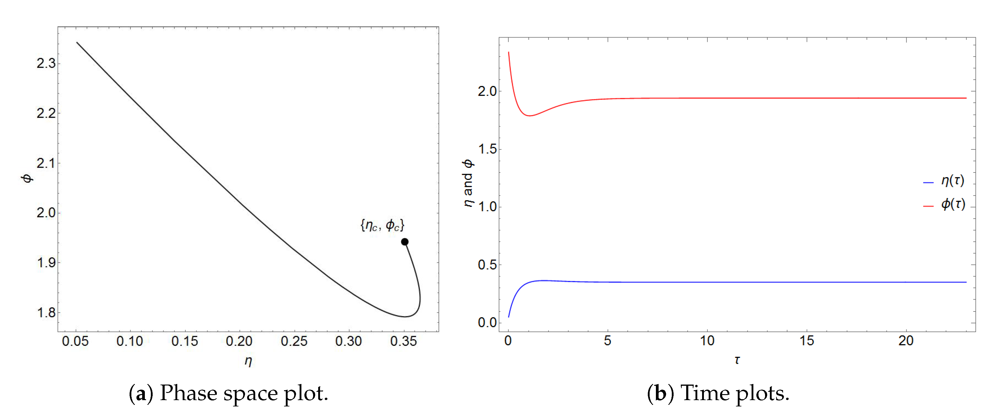
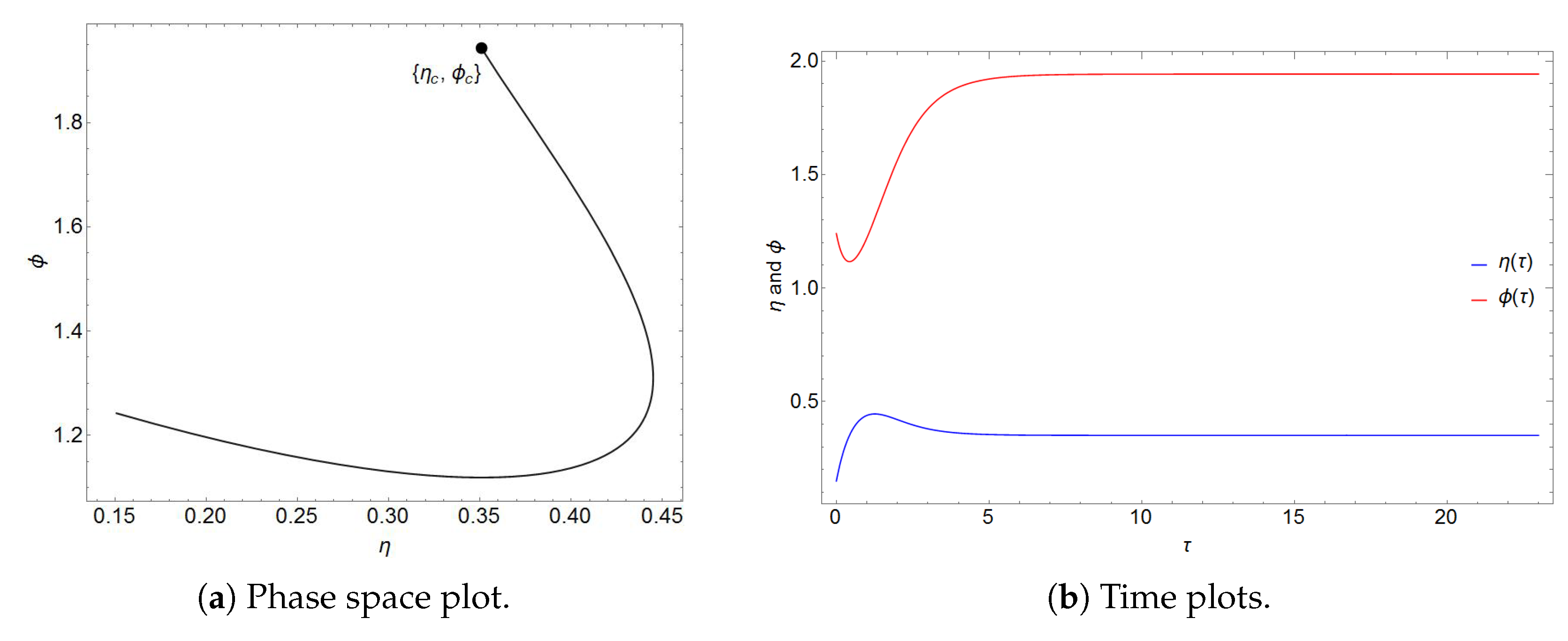
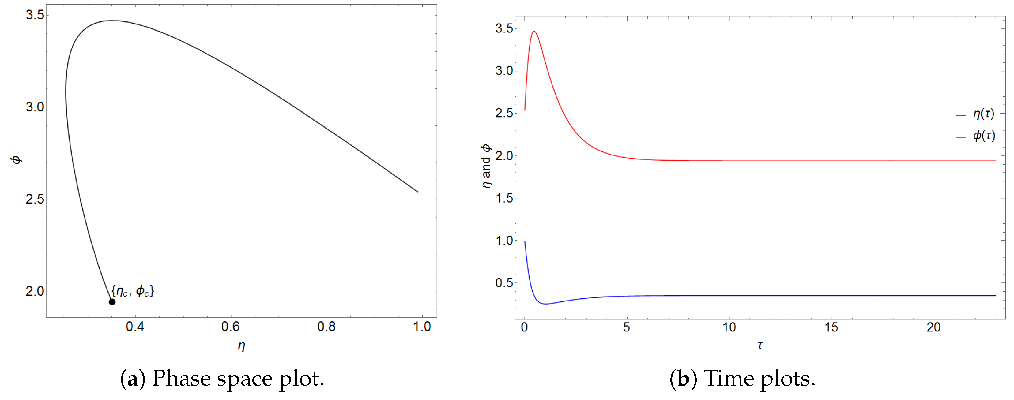
Figure 1, Figure 2 and Figure 3 show numerical simulations of the solutions of Equation (18) by choosing parameters that fulfill the conditions for the stability of the CW point. In all three solutions, the trajectories are asymptotically attracted towards the fixed point $({\eta }_c,{\varphi }_c)$ in the phase space. Additionally, it can be seen that $Q_2$ is an ordinary attractive sink, which is consistent with the analysis from Section 3.1, where it was found that both eigenvalues are real and negative. The time plots show critically damped oscillations towards the equilibrium values ${\eta }_c$ and ${\varphi }_c$ in each case.

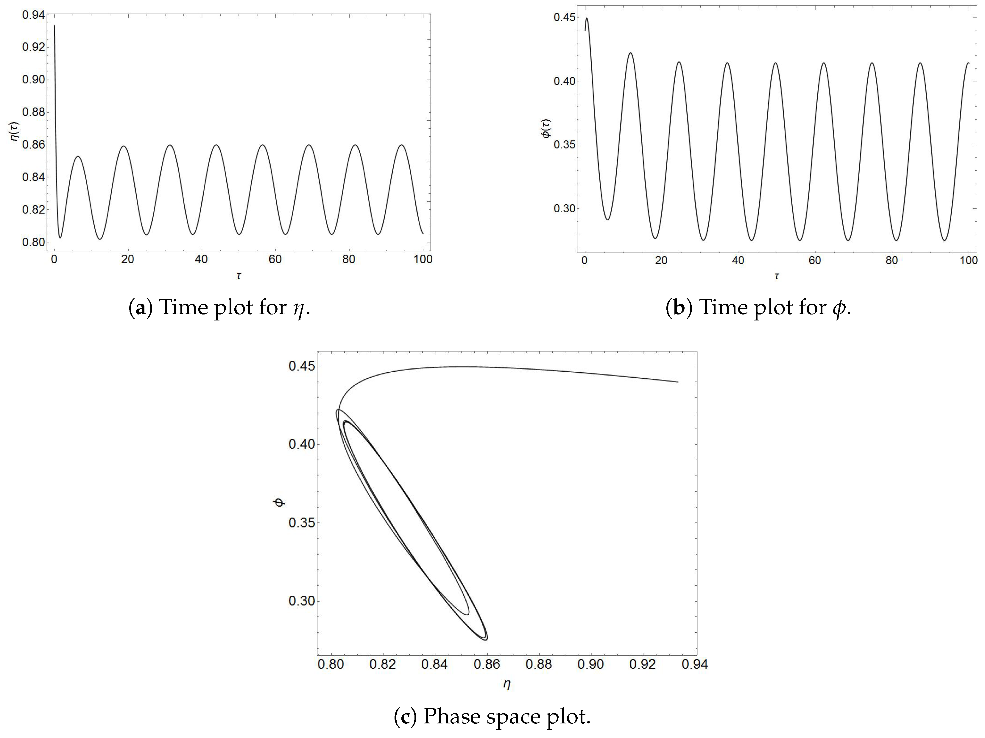
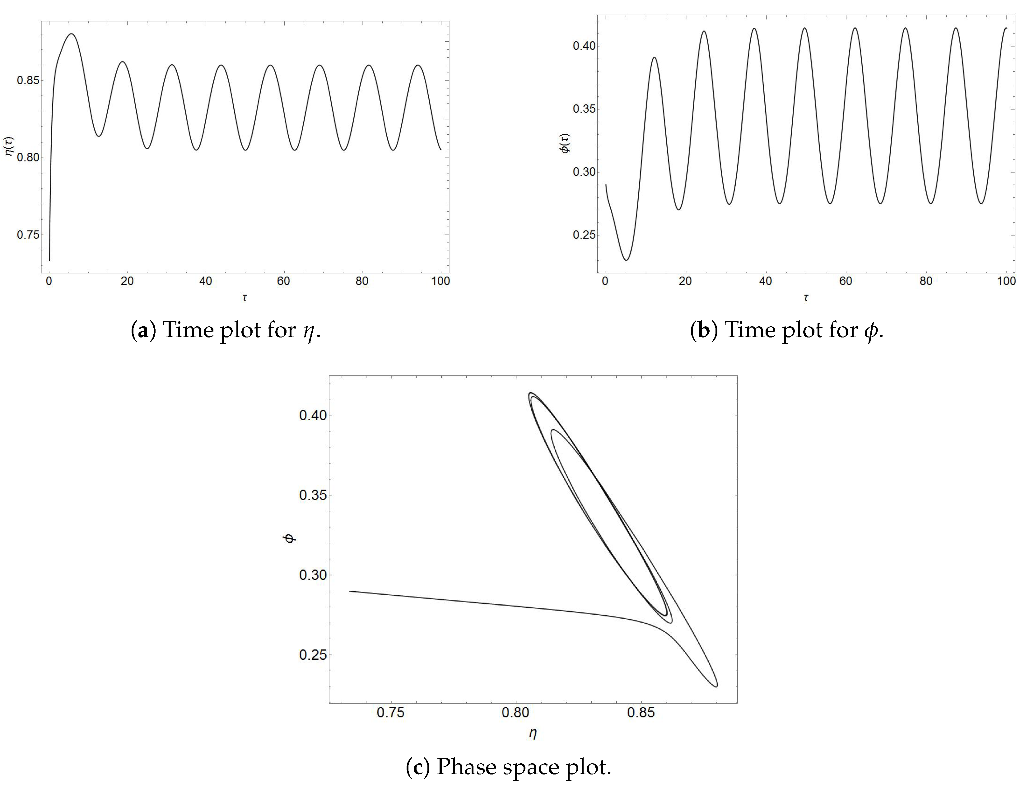
The Q-Switching technique was modeled by assuming a periodic behavior of the quality Q of the cavity. When introducing this sinusoidal term, the Lotka–Volterra model for lasers of Equation (17) turns into a periodically forced system. For simplicity, if the modulation $ϵ$ is small, the system may be approximated as in Equation (39). Thus, the asymptotically stability of the fixed point is transformed into a limit cycle because of the external force acting on the system, which is illustrated in the phase space plots from Figure 4a and Figure 5a. Moreover, the time plots from Figure 4b,c and Figure 5b,c show that the level 2 of the laser is quickly depopulated while the number of emitted photons increases, which will result in intense pulses of light as expected.

6. Conclusions

A set of rate equations for the emitted photons and population inversion in a laser cavity was obtained by making an analogy between predation in population dynamics and stimulated emissions in laser physics. It was shown that the inversion density $\Delta n$ and the emitted photons $\Phi$ may be identified as the predators and the preys, respectively, in Equation (1). However, it was necessary to transform the parameters of the original Lotka–Volterra model to make it suitable for lasers.

The dimensionless form of the obtained rate equations has two critical points: one where lasing stops and another where CW operation is achieved. Lyapunov’s first method yielded the conditions for the instability of the former and the asymptotic stability of the latter. Furthermore, a Lyapunov potential provided the stability regions of the CW operation point.

Finally, the Q-Switching technique was illustrated in the Lotka–Volterra model for lasers by introducing a sinusoidal behavior of the quality Q of the cavity and approximating the resulting equations for a weak modulation $ϵ$. This results in a periodically forced system, which transforms the asymptotically stable fixed point into a limit cycle in the phase space.