1. Introduction
The study of light beam propagation through a turbulent atmosphere has received considerable attention owing to its important applications in free-space optical (FSO) communications, optical imaging and remote sensing [
1,
2,
3,
4]. It is known that atmospheric turbulence varies with geographical environment, season, weather and so on. Different from terrestrial environments, where temperature difference dominates the behaviors of the air’s refractive index fluctuations, in maritime environments, humidity fluctuation is another significant factor that affects optical turbulence, which makes beam propagation more complicated [
5]. In some practical situations, FSO-based information transmission for various purposes on seas/lakes is encountered; for instance, vessel-to-vessel or ship-to-satellite communications. Therefore, knowledge of the interaction of optical beams with the marine atmosphere is of particular importance. In 2008, Grayshan and coworkers developed a new analytical marine atmospheric spectrum as an approximation to Hill’s Salton Sea numerical spectrum [
6]. The spectrum was believed to be general and applicable for marine atmospheric turbulence in other areas. Later, the scintillation expressions of spherical waves using the newly developed spectrum were derived and used to infer path average values of the structure constant [
7]. Since then, much work has been devoted to optical propagation through marine atmospheric turbulence [
8,
9,
10,
11,
12,
13,
14]. The probability density function of the intensity of a Gaussian beam was explored experimentally over water links in [
8]. The spiral spectrum and mode crosstalk of several laser beam modes, including Airy beams, Bessel–Gauss beams and Laguerre–Gaussian beams in weak or moderate to strong marine turbulence, were well investigated [
9,
10,
11,
12,
13]. Meanwhile, the study of optical propagation also extended to marine turbulence in anisotropic or non-Kolmogorov cases [
15,
16,
17,
18].
On the other hand, it has long been known that the use of partially coherent beams as information carriers is one of the effective ways to overcome/reduce the turbulence-induced negative effects in FSO communications [
19,
20]. Through modulating the correlation functions (degree of coherence functions) of partially coherent beams, it provides more freedom to further reduce the scintillation index and beam wander induced by turbulence. It was revealed in [
21] that multi-Gaussian-correlated beams (a special type of partially coherent beams) have advantages over Gaussian Schell-model (GSM) beams for the reduction of turbulence-induced intensity scintillation. The result was later experimentally demonstrated in [
22,
23]. Modulation of the polarization or phase of partially coherent beams to reduce the intensity scintillation index in turbulence was also experimentally demonstrated in [
24,
25,
26]. In [
27], it was shown that nonuniformly correlated (NUC) beams can not only reduce the intensity scintillation but also have a high average received intensity at a certain propagation distance in atmospheric turbulence compared with Schell-model beams.
Just recently, we introduced a new type of random light source, of which the degree of coherence (DOC) is the fourth-order root of a Lorentz–Gaussian function, having linear and cubic-phase terms, named the modified complex Lorentz–Gaussian correlated (MCLGC) beam [
28]. Such a source is capable of producing an Airy-like spectral density pattern in the far field due to its special DOC. In this paper, our aim is to examine the propagation characteristics of MCLGC beam propagation through marine atmospheric turbulence. The propagation formula of spectral density in marine turbulence is derived using the power spectrum introduced in [
6], and the behaviors of spectral density under propagation are investigated in detail through numerical examples. Further, simple analytical expressions for the r.m.s beam width, divergence angle and
M2 factor are also derived based on the Wigner distribution function. The influences of turbulence parameters on the r.m.s beam width and
M2 factor are presented.
2. Spectral Density of a MCLGC Beam Through Marine Atmospheric Turbulence
The cross-spectral density (CSD) function of a MCLGC beam in the source plane (
z = 0) can be expressed as [
28]
with its degree of coherence (DOC)
μx(
xd) or
μy(
yd) being
where
r1 = (
x1,
y1) and
r2 = (
x2,
y2) are two arbitrary position vectors in the source plane, perpendicular to the propagation axis
z.
ω is the radian frequency.
xd =
x2 −
x1 and
yd =
y2 −
y1 are two difference coordinates.
σ0 and
δ0 denote the beam width and the coherence width, respectively.
a0 is a positive real constant that controls the number of side lobes in the far-field spectral density.
is the transverse Gouy phase. For brevity, the dependence of the beam parameters and the derived quantities on the frequency
ω in the following analysis is omitted. Note that the expression for the DOC in Equation (2) is slightly different from that in [
25]. In the present form, the centroid of the beam remains on the
z-axis during free-space propagation.
Within the accuracy of the paraxial approximation, the propagation of a partially coherent beam through atmospheric turbulence can be treated by the extended Huygens–Fresnel (eHF) integral, given by [
19,
20]
where
k = 2π/
λ is a wave number, with
λ being the wavelength of a light beam.
ρ1 and
ρ2 are two position vectors in the output plane.
is the complex phase perturbation (induced by the turbulence) of a spherical wave from the source plane to the output plane. The asterisk and the angle brackets, respectively, stand for the complex conjugate and the ensemble average over the turbulence fluctuations. Suppose that the statistics of the turbulence is isotropic and homogeneous; the second-order statistics of complex phase fluctuations under the Rytov approximation can be expressed as [
1]
where
rd =
r2 −
r1 and
ρd =
ρ2 −
ρ1.
is the power spectrum of the refractive index fluctuations of the turbulence.
, with
κx and
κy denoting the
x and
y components of the spatial frequency, respectively.
J0 is the first type of Bessel function of zero order. In the derivation of Equation (4), the Makov approximation, which assumes that the covariance function of refractive-index fluctuations is a delta-function along the propagation direction, is applied. To further simplify Equation (4), we assume that the points of interest in the beam transverse section are sufficiently close to the propagation axis or transverse coherence width of the laser beam propagating in turbulence is much smaller than the inner scale of the turbulence for a certain propagation distance [
29]. In this case, the Bessel function can be chosen as the first two terms of Taylor expansion, i.e.,
, to a good approximation. On substituting the Taylor expansion into Equation (4) and integrating over
t, it becomes
From Equation (5), if we define a new function
, this result is similar to that of a quadratic approximation provided that
is replaced of
, where
ρ0 is the coherence width of a spherical wave propagating in atmospheric turbulence under Kolmogorov spectrum condition, i.e.,
. It is known that the eHF integral and quadratic approximation are valid for both weak and strong turbulence [
1,
30]. According to [
6], the power spectrum of marine atmospheric turbulence can be written as
where
;
l0 and
L0 are the inner scale size and outer scale size of the turbulence.
Cn2 is the structure constant, which almost remains invariant along the horizontal direction. On substituting Equation (6) into the integral term in Equation (5) and integrating over
κ, it turns out to be
where
and
are the incomplete Gamma function and confluent hypergeometric function, respectively. In general, the inner scale size
l0 is far smaller than the outer scale size
L0, i.e.,
κH >>
κ0. Equation (7) can be expressed as the following approximate expression through remaining the first two terms of Tylor expansion of the incomplete Gamma function and the hypergeometric function
Note that Equation (8) is valid if the condition
l0 <<
L0 is satisfied. On substituting Equations (1) and (5) into Equation (3), and introducing the “sum” and “difference” coordinates
we obtain the expression after arrangement
with
has the same form as
with “
x” in place of “
y.” If we only focus on the evolution properties of spectral density in the marine atmosphere, i.e.,
, it can be written as the following Fourier transform form after integrating over
xs(
ys)
with
where
FT denotes the Fourier transform. Equation (12) provides a convenient way to evaluate the spectral density of the MCLGC beam propagation in turbulence. It follows from Equation (12) that the spectral density is a rather simple Fourier transform of the product of the DOC and the Gaussian function with width
w. Let us now analyze the propagation characteristics of the MCLGC beam in turbulence through numerical examples based on the derived Equation (12).
In the numerical calculation, the beam parameters and turbulence parameters are chosen to be
σ0 = 10 mm,
δ0 = 2 mm,
λ = 632.8 nm,
a0 = 0.1,
l0 = 1 mm and
L0 = 1 m, and they are kept fixed unless other values are specified.
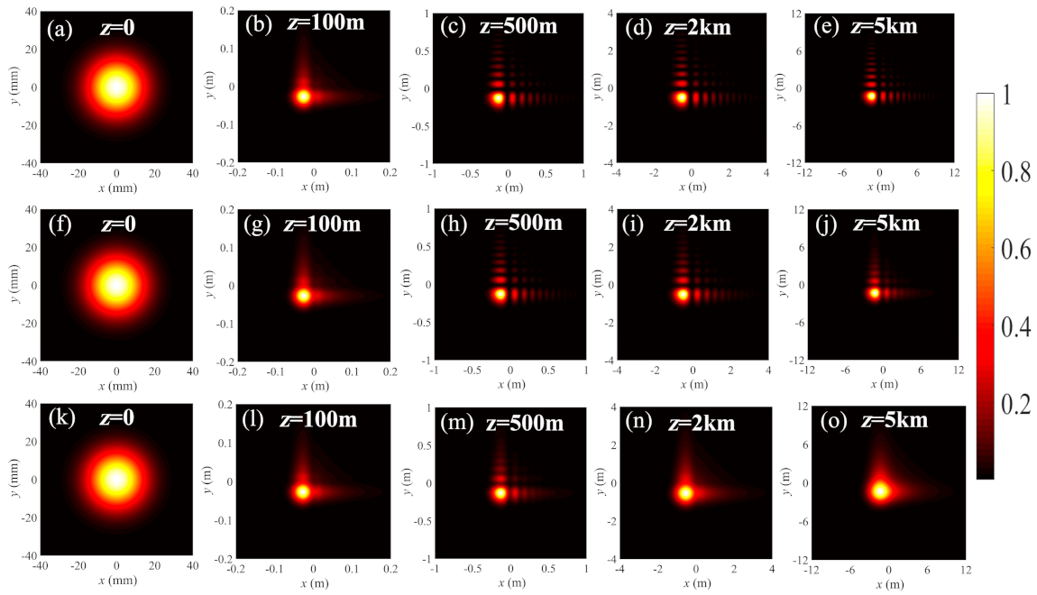
Figure 1 illustrates the density plots of the normalized spectral density of the MCLCG beam propagation in the marine turbulence with different structure constants
Cn2. For comparison, the spectral density in the free-space propagation (
Cn2 = 0) is also plotted (see
Figure 1a–e). The beam profile gradually turns from a Gaussian shape in the source plane to an Airy-like pattern as the propagation distance increases. When the propagation distance is larger than
z = 500 m, the beam profile remains invariant on further propagation except the beam size enlarges due to diffraction effects. In the presence of turbulence, the spectral densities in the first 100 m propagation distance for
Cn2 = 5×10
–14m
–2/3 and
Cn2 = 5×10
–13m
–2/3 are almost the same compared to that in the free space. This is because the effects of optical turbulence on the beam propagation do not occur suddenly, it accumulates gradually with the increase of propagation distance and appears gradually. For the first 100 m propagation distance, one could estimate the strength of turbulence via the Rytov variance
. The calculated values of
σ2 for
Cn2 = 5×10
–14m
–2/3 and
Cn2 = 5×10
–13m
–2/3 are 0.0416 and 0.416, respectively. This range falls into weak turbulence. On the other hand, partially coherent beams with a low coherence width are less affected by the turbulence-induced degeneration. As a result, in the first 100 m propagation, the spectral densities between
Cn2 = 5×10
–14m
–2/3 and
Cn2 = 5×10
–13m
–2/3 are almost the same with that without turbulence. However, as the propagation distance further increases, the effects of turbulence appear. In the case of
Cn2 = 5×10
–13m
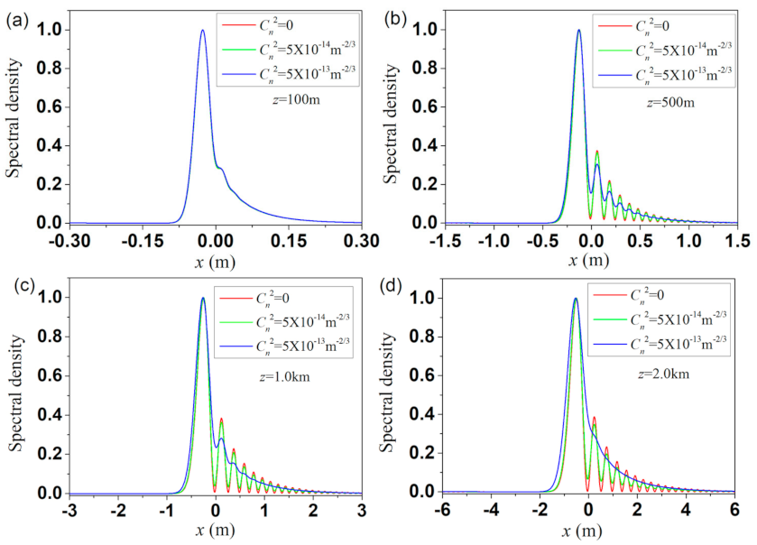
–2/3, the side lobes become a little fuzzy at 1 km propagation distance or up to 2 km distance. To clearly see the variance of the spectral density with different structure constants, we plot in
Figure 2 the 1D spectral density
Sx(
ρx,
z) corresponding to those in
Figure 1. One can see that the side lobes diminish with the increase of the strength of turbulence at a certain propagation distance.
The aforementioned propagation features of the MCLGC beam in marine turbulence can be explained explicitly with the help of the derived formula of Equation (12). It is shown in Equation (12) that the propagated spectral density is determined by the Fourier transform of the product of a Gaussian function exp(–
αd2/
w2) and the DOC function of the beam. The width
w of the Gaussian function
w shown in Equation (13) can be divided into three parts, i.e., the first, second and third terms in parentheses are the contributions from the initial beam width, diffraction effect and turbulence effect, respectively.
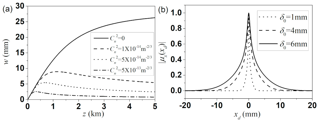
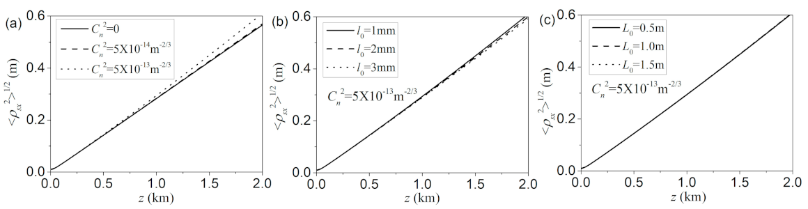
Figure 3a illustrates the variation of
w as a function of the propagation distance with different strengths of turbulence. In the absence of turbulence (
T = 0, see the solid curve in
Figure 3a),
w increases monotonously from 0 to a stable value
as the beam leaves from the source plane. On the other hand, the width of the DOC is mainly dependent on the coherence width
δ0. Therefore, when the propagation distance is short, the size of the Gaussian function is much smaller than that of the DOC. In this case, the Gaussian function plays a central role in the product of the Gaussian function and the DOC function. As a consequence, the spectral density is nearly of Gaussian shape. As the width
w increases with the increase of propagation distance until it reaches a stable value, the DOC gradually plays the key role in the product under the condition that the coherence width
δ0 is far smaller than
. The spectral density of the beam becomes the Fourier transform of the DOC function, i.e., an Airy-like pattern, and then keeps the profile unchanged for further propagation (see
Figure 1a–e).
In the presence of turbulence, the situation is somewhat different. Following from Equation (13), the third term is caused by turbulence, where
T is closely dependent on the power spectral density. When the propagation distance is short or the turbulence is weak, the effect of the turbulence is negligible. This is why the spectral density in the first 100 m propagation shown in
Figure 1 in the free space and turbulence are almost the same. However,
w will decrease for a sufficient large propagation distance due to the effects of turbulence. Hence, the Airy-like spectral density blurs again in turbulence, which is quite different from the case in free space. From Equation (12), one can also explain why a partially coherent beam with small coherence width is less affected by the turbulence. The reason is that the DOC only depends on the coherence width, and the distribution of DOC becomes narrow as the coherence width decreases (shown in
Figure 3b). Hence, for the same value of
w (same condition of the turbulence, propagation distance and initial beam width), the DOC function with a small coherence width is more likely to retain its original form when it is apodized by the function exp(–
αd2/
w2).
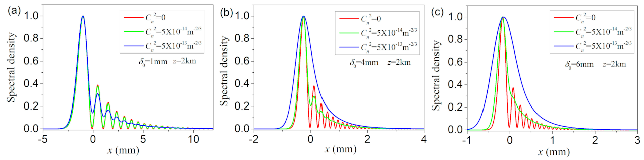
Figure 4 presents the 1D normalized spectral density with different coherence widths at propagation distance
z = 2 km. As expected, the spectral density with
δ0 = 1 mm is less affected by the turbulence compared to those with
δ0 = 4 and 6 mm. Though our result is obtained from the propagation of the MCLGC beam, it also can be extended to other types of partially coherent beams.
We now pay attention to the effect of the light wavelength on the behavior of spectral density in marine turbulence.
Figure 5 presents the 1D spectral densities of the MCLCG beam with different wavelengths at several propagation distances. The structure constant used in the simulation is
Cn2 = 5×10
–13m
–2/3. As expected, the beam size with a long wavelength is larger than that with a short wavelength. In addition, the transition of the spectral density with a long wavelength from the Gaussian profile to an Airy-like pattern becomes fast on propagation (see
Figure 5a). One can also see from
Figure 5b–d that the spectral density with a long wavelength is more likely to keep the Airy-like pattern in turbulence. As shown in
Figure 5d, the side lobes in the spectral density with
λ = 632.8 nm disappear, whereas it is also observable in the case of
λ = 1310 or 1550 nm. The reason can be seen from the third term (turbulence = effected term) in Equation (13), i.e.,
π2k2Tz/3, the longer wavelength corresponds to the smaller value of wavenumber
k, which weakens the effect of turbulence.
To assess the influences of optical turbulence on the spectral densities during propagation in turbulence, a parameter
D is used to characterize it, defined as [
31]
The subscript “
free” and “
tur” denote the spectral density at propagation distance
z without and with turbulence. According to the definition, the upper and lower limits of
D are 1 and 0, respectively. The larger the value
D is, the less the spectral density is affected by the turbulence.
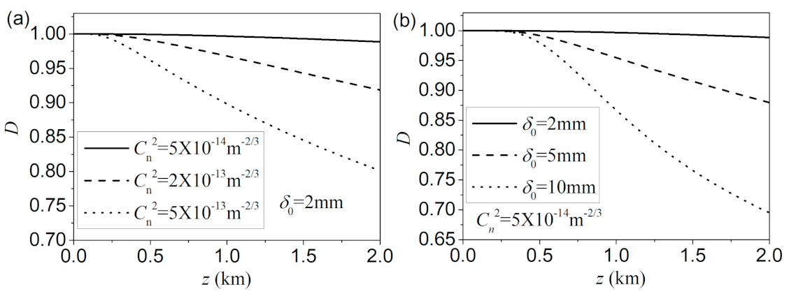
Figure 6 illustrates the dependence of parameter
D on the propagation distance with different structure constants and different initial coherence widths. It can be seen from
Figure 6a that as the strength of turbulence increases, the
D drops fast with the increase of propagation distance, implying that the spectral density of the MCLGC beam suffers more serious distortion in strong turbulence.
Figure 6b indicates that the MCLGC beam with small initial coherence width is more likely to resist the effect of turbulence from the point of view of spectral density.
3. R.m.s Beam Width, Divergence Angle and Propagation Factor of MCLGC Beams in Marine Atmospheric Turbulence
R.m.s beam width, divergence angle and propagation factor (M2 factor) are three important parameters to characterize the characteristics of a laser beam under propagation. Especially for the propagation factor, it is currently used in the data sheet of commercial lasers. The random fluctuations of the refractive index induced by the turbulence will cause the beam’s random displacement, scintillation of intensity and decrease of coherence during propagation. As a consequence, the r.m.s beam width and divergence angle increase, and the propagation factor deteriorates in the presence of turbulence.
In this section, we will first derive the second-order moments of MCLGC beam propagation in marine turbulence based on the Wigner distribution function and then investigate the evolution of the r.m.s beam width, divergence angle and propagation factor through numerical examples.
According to [
32,
33], the Wigner distribution function of the MCLGC beam at propagation distance
z in turbulence can be expressed as
where
is the CSD function of the MCLGC beam in turbulence at distance
z, shown in Equations (10)–(11).
Θ = (
θx,
θy) denotes the divergence angle with respect to the mean propagation z-axis. To evaluate Equation (15), we write the CSD function of the MCLGC beam in the source plane as the following integral form
where
takes the form
On substituting Equations (10) and (16) into Equation (15), we obtain the expression
Integrating over
rs and
rd in Equation (18), it turns out to be
On substituting Equation (17) into Equation (19) and integrating over
, the Wigner distribution function finally becomes
With the help of the Wigner distribution function, the arbitrary moments of the MCLGC beam in turbulence can be written as
with
where
I denotes the total energy carried by a light beam.
n1,
n2,
m1 and
m2 are the integral numbers. Here, we focus on the propagation features of the second-order moments, which means that
n1 +
n2 +
m1 +
m2 = 2. On substituting Equation (20) into Equation (21), and after straightforward integrating, we obtain analytical expressions for the ten second-order moments of the MCLGC beam in turbulence
where
denotes the diffraction coefficient.
and
represent the r.m.s beam width along the
x- and
y-directions, respectively. The first term in Equation (23) is the contribution from the initial beam width; the second term and the third term denote diffraction-induced and turbulence-induced beam spreading, respectively. One finds that not only the initial beam width and coherence width, but also the parameter
a0 will affect the diffraction-induced beam spreading. The smaller value the parameter
a0 (the more side lobes), the larger the r.m.s beam width.
and
are the r.m.s divergence angle of the MCLGC beam in turbulence. The cross-moments
and
are closely related to the propagation factor and the effective radius curvature under propagation. It is found that the other two cross-moments
and
remain zero invariant on propagation, implying that the total orbital angular moment is zero and is conserved on propagation.
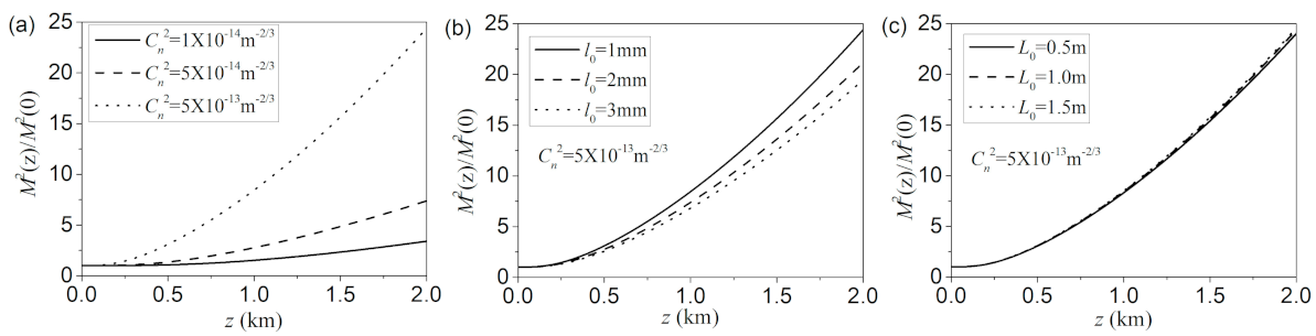
Figure 7 illustrates the variation of the r.m.s beam width along the
x-direction with the propagation distance for different structure constants, inner scale sizes and outer scale sizes. As expected, the beam width spreads much faster with the increase of the strength of turbulence. The inner scale size has also a certain effect on the beam spreading, whereas the outer scale size has almost no effect on the beam spreading. As the inner scale size decreases, the beam spreading becomes fast. This can be explained by the fact that the small inner scale size tends to make the beam spot into small speckles. Each speckle has a small beam width compared to the whole beam spot, which makes the beam width spread fast. The main effect of the outer scale on the beam is to randomly deviate the beam propagation direction with the respective z-axis, known as beam wander. This beam wander is too small compared to the r.m.s beam width at that propagation distance. As a result, the outer scale size has little effect on beam spreading.
The beam propagation factor
M2, also called the beam quality factor, is a significant parameter to characterize the beam propagation properties in many practical applications. On the basis of the second-order moments, the
M2 factor can be written in the following form
On substituting Equations (23)–(25) into Equation (27), the
M2 of the MCLGC beam in marine turbulence takes the form
with
where
M2(0) is the
M2 factor of the MCLGC beam in the source plane. A smaller initial coherence width and parameter
a0 will lead to an increase in the
M2 factor. It follows from Equation (28) that in the absence of turbulence (
T = 0), the
M2 factor is independent of the propagation distance, indicating that it remains invariant on free-space propagation. In the presence of turbulence, the
M2 factor increases/deteriorates during propagation due to the effect of turbulence.
Figure 8 presents the variation of the normalized
M2 factor
M2(z)/
M2(0) with the propagation distance for different structure constants, inner scale sizes and outer scale sizes. The evolution behaviors are similar to those with the r.m.s beam width shown in
Figure 7. Nevertheless, the increases in the
M2 factor with propagation distance seem much more rapid than those of r.m.s beam widths as the strength of turbulence increases or the inner scale size decreases. This is because the r.m.s beam width and the r.m.s divergence angle increase simultaneously for the large values of structure constants and small values of inner scale sizes.


