Article

Spiral Caustics of Vortex Beams

by
Viktor A. Soifer
1,2,
Sergey I. Kharitonov
1,2,
Svetlana N. Khonina
1,2,*,
Yurii S. Strelkov
1 and
Alexey P. Porfirev
1,2
1
Department of Technical Cybernetics, Samara National Research University, Moskovskoye Shosse 34, 443086 Samara, Russia
2
IPSI RAS—Branch of the FSRC “Crystallography and Photonics” RAS, Molodogvardeyskaya 151, 443001 Samara, Russia
*
Author to whom correspondence should be addressed.
Photonics 2021, 8(1), 24; https://doi.org/10.3390/photonics8010024
Submission received: 18 December 2020 / Revised: 14 January 2021 / Accepted: 15 January 2021 / Published: 19 January 2021

Abstract

:
We discuss the nonparaxial focusing of laser light into a three-dimensional (3D) spiral distribution. For calculating the tangential and normal components of the electromagnetic field on a preset curved surface we propose an asymptotic method, using which we derive equations for calculating stationary points and asymptotic relations for the electromagnetic field components in the form of one-dimensional (1D) integrals over a radial component. The results obtained through the asymptotic approach and the direct calculation of the Kirchhoff integral are identical. For a particular case of focusing into a ring, an analytical relation for stationary points is derived. Based on the electromagnetic theory, we design and numerically model the performance of diffractive optical elements (DOEs) to generate field distributions shaped as two-dimensional (2D) and 3D light spirals with the variable angular momentum. We reveal that under certain conditions, there is an effect of splitting the longitudinal electromagnetic field component. Experimental results obtained with the use of a spatial light modulator are in good agreement with the modeling results.

Graphical Abstract

1. Introduction

In the classical geometric optics light is assumed to propagate along light rays, which are straight lines in a uniform medium. One of the amazing phenomena in the geometric optics is the formation of caustics, which are formed as an envelope of optical rays. The geometric optics [1,2] can be looked at as the short-wave limit of the classical optics, with the latter relying on the asymptotic approximation of Maxwell’s equations [2]. In the basis of short-wave asymptotics is the fact that the electromagnetic field is described by integrals of rapidly oscillatory functions.
To determine a light ray intensity, a vector Kirchhoff integral needs to be taken. The common assumption of the geometric optics that the intensity at a given point is only determined by an insignificant fragment of the diffractive optical element (DOE) is its pivotal point. In many cases, an increase in the integration region does not lead to a considerable change in the intensity at the observation point. In terms of mathematics, this fact is described by a stationary phase method [2]. However, the diffraction integral not always can be calculated with the stationary phase method as in some cases, its use leads to the appearance of irremovable singularities, with the electromagnetic field intensity at the point tending to infinity. This is what happens in the neighborhood of geometric caustics. Caustics have been studied in numerous works. In the general case, classification of all possible caustics was conducted by V. I. Arnold [3]. The use of the catastrophe theory in the study of caustics is reported in Refs. [4,5]. An approach alternative to that based on the integral representations of rapidly oscillatory functions is discussed in Ref. [6], where the Helmholtz equation is reduced to the solution of a chain of differential equations. The method is analogous to reducing the Helmholtz equation to the solution of an eikonalequation and a transfer equation.Although it has some advantages, this approach only allows one to find the field in the neighborhood of non-singular caustics. Asymptotic methods for analyzing equations and the field near singular points are set forth in Refs. [7,8,9,10]. In this work, we study caustics of spiral vortex beams. The vortex beams are special in that the ray structure of their field depends on the wavelength [11]. Unlike Ref. [11], where classical vortex beams that form axisymmetric caustics were studying, in this work, we look into light fields with a spiral caustic.
Optical elements capable of generating spiral intensity patterns have been treated in a number of works [12,13,14,15,16,17,18,19,20,21,22,23,24]. In particular, E. Abramochkin and V. Volostnikov [12,13] proposed generating plane curves by means of astigmatic transforms. In Ref. [14], a carrier frequency method in combination with several parabolic wavefronts was applied to generating free-form 3D intensity distributions composed of light spots. A similar approach based on the superposition of diffraction-free beams, the spatial spectrum of which is determined on a narrow ring, was discussed in Refs. [15,16,17] for shaping different 3D light curves. A special combination of conical and vortex phases [18,19] makes it possible to form a light spiral in the focal plane of a lens. Note that conventional diffractive spiral axicons [20] and more complex refractive analogs [21] can be used to generate 3D spiral intensity in the near diffraction zone. The simplest optical element for shaping a spiral intensity distribution is a power-exponent phase plate [22,23] or a generalized spiral phase plate [24].
In this work, we propose DOEs with special angular dependence structure to generate 2D and 3D light spirals with the variable angular momentum. The considered approach expands the family of beams with optical vortices, which have found their applications in various fields including optical manipulation and laser structuring [25,26,27,28,29,30,31,32].

2. Electromagnetic Field on a Curved Surface

When tackling the problem of diffraction by a 3D solid (e.g., a ball, a cylinder, etc.) bounded by a curved surface, the tangential components of the electromagnetic field need to be joined/stitched [33,34,35,36,37]. Below, we discuss an asymptotic method for calculating the tangential and normal components of the electromagnetic field on a free-shape curved surface.

2.1. Coordinate Systems

Hereinafter, we utilize the following coordinate systems.
The Cartesian coordinates ( u , v , 0 ) on the DOE under study and the Cartesian coordinates ( x , y , z ) in the field computation domain.
The polar coordinates ( ρ 0 , θ 0 , 0 ) on the DOE under study:
u = ρ 0 cos θ 0 , v = ρ 0 sin θ 0 .
The cylindrical coordinates ( ρ , θ , z ) in the field computation domain:
x = ρ cos θ , y = ρ sin θ , z = z .
Although the cylindrical coordinates are widely used, there are problems where the field needs to be analyzed in the local coordinates on a more complex-shaped surface. One such problem deals with calculating light forces exerted upon a free-shape solid.
Because of this, in a more general case, the surface of interest will be described by parametric equations:
x = X ( ξ , η ) , y = Y ( ξ , η ) , z = Z ( ξ , η ) .

2.2. An Incident Wave in the Coordinates ( x , y , z )

The electric field of a plane wave may be given by
E ( x , y , z ) = ( E x ( α , β ) E y ( α , β ) E z ( α , β ) ) exp [ i ( α x + β y + γ ( α , β ) z ) ]
where ( α , β ) are the spatial spectral coordinates linked with the Cartesian coordinates ( x , y , z ) , E j ( α , β ) is the j-th component of the spatial spectrum of the electric field.
E z ( α , β ) = γ 1 ( α , β ) ( α E x ( α , β ) + β E y ( α , β ) )
In these coordinates, the electric field of an incident plane wave on the surface of interest takes the form:
E ( ξ , η ) = [ E ξ ( α , β ) E η ( α , β ) E N ( α , β ) ] = P ( ξ , η ) ( E x ( α , β ) E y ( α , β ) E z ( α , β ) ) × × exp { i [ α X ( ξ , η ) + β Y ( ξ , η ) + γ ( α , β ) Z ( ξ , η ) ] } ,
P ( ξ , η ) = ( X ( ξ , η ) ξ Y ( ξ , η ) ξ Z ( ξ , η ) ξ X ( ξ , η ) η Y ( ξ , η ) η Z ( ξ , η ) η N x ( ξ , η ) N y ( ξ , η ) N z ( ξ , η ) )
where the matrix elements in (7) contain parametric equations that describe the surface in (3) and N j ( ξ , η ) are the components of the normal vector to the surface.
The electric field of a plane wave may also be defined as
E ( x , y , z ) = ( E T M Z ( α , β ) , E T E Z ( α , β ) ) × × ( A ( α , β ) B ( α , β ) ) exp [ i ( α x + β y + γ z ) ] ,
E T M Z ( α , β ) = ( γ α γ β ( k 0 2 ε μ γ 2 ) ) , E T E Z ( α , β ) = ( k 0 μ β k 0 μ α 0 )
where k 0 = 2 π / λ 0 is the wavenumber for the wavelength of light λ 0 in vacuum and ε , μ are the dielectric permittivity and magnetic permeability of the medium.
The functions A ( α , β ) , B ( α , β ) define the contribution of the TM- and TE-components of the electromagnetic field. These may be replaced with functions E x ( α , β ) , E y ( α , β ) , which are given by
( E x ( α , β ) E y ( α , β ) ) = ( γ α k 0 μ β γ β k 0 μ α ) ( A ( α , β ) B ( α , β ) )
( A ( α , β ) B ( α , β ) ) = ( γ α k 0 μ β γ β k 0 μ α ) 1 ( E x ( α , β ) E y ( α , β ) )
In these coordinates, the electric field may also be represented as
E ( ξ , η ) = P ( ξ , η ) E T M E ( α , β ) ( A ( α , β ) B ( α , β ) ) × × exp { i [ α X ( ξ , η ) + β Y ( ξ , η ) + γ ( α , β ) Z ( ξ , η ) ] } ,
E T M E ( α , β ) = ( E T M Z ( α , β ) , E T E Z ( α , β ) )
In the Cartesian coordinates, the magnetic field takes the form:
H ( x , y , z ) = ( H T M Z ( α , β ) , H T E Z ( α , β ) ) × × ( A ( α , β ) B ( α , β ) ) exp [ i ( α x + β y + γ z ) ] ,
H T M Z ( α , β ) = ( k 0 ε β k 0 ε α 0 ) , H T E Z ( α , β ) = ( γ α γ β ( k 0 2 ε μ γ 2 ) )
In the coordinates linked with the surface of interest, the magnetic field is given by
H ( ξ , η ) = [ H ξ ( α , β ) H η ( α , β ) H N ( α , β ) ] = P ( ξ , η ) H T M E ( α , β ) ( A ( α , β ) B ( α , β ) ) × × exp { i [ α X ( ξ , η ) + β Y ( ξ , η ) + γ ( α , β ) Z ( ξ , η ) ] } ,
H T M E ( α , β ) = ( H T M Z ( α , β ) , H T E Z ( α , β ) )

2.3. Computation of the Field: General Case

In the general case of a field composed of superposition of plane waves, the field on the surface is described by the expression:
( E ( ξ , η ) H ( ξ , η ) ) = P ( ξ , η ) ( E T M E ( α , β ) H T M E ( α , β ) ) ( A ( α , β ) B ( α , β ) ) × × exp { i [ α X ( ξ , η ) + β Y ( ξ , η ) + γ ( α , β ) Z ( ξ , η ) ] } d α d β ,
where the functions A ( α , β ) , B ( α , β ) are expressed using Equation (11) through the transverse components of the spatial spectrum, E x ( α , β ) , E y ( α , β ) .
The spatial spectrum is derived from a Fourier transform of the transverse components of the electric field on the DOE:
( E x ( α , β ) E y ( α , β ) ) = 1 4 π 2 ( E x ( u , v ) E y ( u , v ) ) exp [ i ( α u + β v ) ] d u d v .
Then, the field on the surface takes the form:
W ( ξ , η ) = ( E ( ξ , η ) H ( ξ , η ) ) = 1 4 π 2 P ( ξ , η ) × × ( E T M E ( α , β ) H T M E ( α , β ) ) ( γ α k 0 μ β γ β k 0 μ α ) 1 ( E x ( u , v ) E y ( u , v ) ) × × exp { i [ α ( X ( ξ , η ) u ) + β ( Y ( ξ , η ) v ) + + γ ( α , β ) Z ( ξ , η ) ] } d α d β d u d v .
In the general case, the relations in (20) may be rewritten as:
W ( ξ , η ) = 1 4 π 2 ( K ( α , β , ξ , η ) , L ( α , β , ξ , η ) ) × × ( E x ( u , v ) E y ( u , v ) ) exp { i [ α ( X ( ξ , η ) u ) + β ( Y ( ξ , η ) v ) + + γ ( α , β ) Z ( ξ , η ) ] } d α d β d u d v ,
where K , L are the column-vectors.
Equation (21) may be given in a different form:
W ( ξ , η ) = G ( ξ , η , u , v ) ( E x ( u , v ) E y ( u , v ) ) d u d v ,
where the matrix G is defined as follows:
G ( ξ , η , u , v ) = 1 4 π 2 ( K ( α , β , ξ , η ) , L ( α , β , ξ , η ) ) × × exp { i [ α ( X ( ξ , η ) u ) + β ( Y ( ξ , η ) v ) + γ ( α , β ) Z ( ξ , η ) ] } d α d β .
Integral (23) can be calculated using a stationary phase method:
G ( ξ , η , u , v ) = = i k 2 π ( K ( k α s , k β s , ξ , η ) , L ( k α s , k β s , ξ , η ) ) z R 1 exp ( i k R 1 ) R 1
where
R 1 = ( X ( ξ , η ) u ) 2 + ( Y ( ξ , η ) v ) 2 + Z 2 ( ξ , η )
α s , β s are derived from the solution of a stationary point equation:
{ α s = ( X ( ξ , η ) u ) ( X ( ξ , η ) u ) 2 + ( Y ( ξ , η ) v ) 2 + z 2 , β s = ( Y ( ξ , η ) v ) ( X ( ξ , η ) u ) 2 + ( Y ( ξ , η ) v ) 2 + z 2 .

3. Computing the Field in the Neighborhood of a Spiral Caustic Surface

An interesting type of light caustics is a spiral. Light spirals can find uses not only for trapping, guiding, and micromanipulation of microparticles [17,29], but also for laser-aided surface structuring [19,38].
Let us analyze a wavefront that has 3D caustics, whose eikonal function may be generally written as:
Ψ ( ρ 0 , θ 0 ) = ( ρ 0 r 0 ( θ 0 ) ) 2 + f 2 ( θ 0 )
where the functions r 0 ( θ 0 ) and f ( θ 0 ) characterize the type of the 3D spiral.
Additional vortex phase singularity exp ( i m θ 0 ) in (27) lets us obtain a vortex spiral wavefront. The vortex component guarantees the intensity null on the optical axis [11,39,40].
The complex amplitude of the electromagnetic field in the initial plane (z = 0) is given by
( E x ( u , v ) E y ( u , v ) ) = ( E x ( ρ 0 ) E y ( ρ 0 ) ) exp [ i k Ψ ( ρ 0 , θ 0 ) ] exp ( i m θ 0 )
Introducing the cylindrical coordinates in the observation plane:
X ( ρ , θ ) = ρ cos θ , Y ( ρ , θ ) = ρ sin θ , Z ( ρ , θ ) = z .
expressions for the Cartesian components of the field may be written in the form:
E x , y ( ρ , θ , z ) = i k 2 π E x , y ( ρ 0 ) z R 1 × × exp { i k [ R 1 + Ψ ( ρ 0 , θ 0 ) ] + i m θ 0 } R 1 ρ 0 d ρ 0 d θ 0 ,
E z ( ρ , θ , z ) = = i k 2 π [ E x ( ρ 0 ) ρ cos θ ρ 0 cos θ 0 R 1 + E y ( ρ 0 ) ρ sin θ ρ 0 sin θ 0 R 1 ] × × exp { i k [ R 1 + Ψ ( ρ 0 , θ 0 ) ] + i m θ 0 } R 1 ρ 0 d ρ 0 d θ 0 ,
where
R 1 = ρ 2 + ρ 0 2 2 ρ 0 ρ cos ( θ 0 θ ) + z 2

3.1. Asymptotic Relations for the Diffraction Integral in the Neighborhood of a Spiral Caustic

In this section, we calculate the field in the neighborhood of a caustic surface, which is defined by parametric equations [11,41]:
{ ρ = ( ρ 0 + S Φ ρ ( ρ 0 , θ 0 ) ) 2 + ( 1 ρ 0 S Φ θ ( ρ 0 , θ 0 ) ) 2 , θ = θ 0 T ( ρ 0 , θ 0 ) , z ( ρ , θ ) = S 2 + 2 ρ ρ 0 cos [ θ 0 T ( ρ 0 , θ 0 ) ] ρ 0 2 ρ 2 ,
where
T ( ρ 0 , θ 0 ) = A t a n ( 1 ρ 0 S Φ θ ( ρ 0 , θ 0 ) , ρ + S Φ ρ ( ρ 0 , θ 0 ) )
and S is the solution of a quadratic equation:
{ S Φ ρ ρ ( ρ 0 , θ 0 ) + [ 1 Φ ρ 2 ( ρ 0 , θ 0 ) ] } × × { S Φ θ θ ( ρ 0 , θ 0 ) + [ ρ ( ρ + S Φ ρ ( ρ , θ ) ) Φ θ 2 ( ρ 0 , θ 0 ) ] } { S Φ ρ θ ( ρ 0 , θ 0 ) + [ Φ θ ( ρ 0 , θ 0 ) ρ S + Φ ρ ( ρ 0 , θ 0 ) Φ θ ( ρ 0 , θ 0 ) ] } 2 = 0 .
May the relations for r 0 ( θ 0 ) and f ( θ 0 ) be linear:
r 0 ( θ 0 ) = r 0 + θ 0 2 π ( r 1 r 0 )
f ( θ 0 ) = f 0 + θ 0 2 π ( f 1 f 0 )
A stationary point relative to the angle θ s will be derived from the equation:
m k ρ 0 ρ sin ( θ θ s ) R s ( ρ 0 , θ s ) + + 1 2 π ( r 0 ( θ s ) ρ 0 ) ( r 1 r 0 ) + f ( θ s ) ( f 1 f 0 ) Ψ ( ρ 0 , θ s ) = 0 .
In this case, the field components in (30) and (31) take the form:
E x , y ( ρ , θ , z ) i k 2 π s exp ( i σ s ) × × E x , y ( ρ 0 ) z R s exp [ i k R s + Ψ ( ρ 0 , θ s ) + i m θ s ] R s × × 2 π k ( R s + Ψ ( ρ 0 , θ s ) ) ρ 0 d ρ 0 ,
E z ( ρ , θ , z ) i k 2 π s exp ( i σ s ) × × [ E x ( ρ 0 ) ρ cos θ ρ 0 cos θ s R s + E y ( ρ 0 ) ρ sin θ ρ 0 sin θ s R s ] × × exp [ i k R s + Ψ ( ρ 0 , θ s ) + i m θ s ] R s 2 π k ( R s + Ψ ( ρ 0 , θ s ) ) ρ 0 d ρ 0 ,
where σ s = ± π / 4 [2],
R s = ρ 2 + ρ 0 2 2 ρ 0 ρ cos ( θ s θ ) + z 2
R s = 2 R s θ 2 = ρ 0 ρ cos ( θ s θ ) R s ( ρ 0 ρ ) 2 sin 2 ( θ s θ ) R s 3
Ψ ( ρ 0 , θ s ) = 1 2 π [ r 0 ( θ s ) ρ 0 ] ( r 1 r 0 ) + f ( θ s ) ( f 1 f 0 ) Ψ ( ρ 0 , θ s )
The expressions in Equations (39) and (40) are 1D integrals. We note that without the use of an asymptotic approach, it is not possible to reduce the Kirchhoff integral to a 1D integral even if both the field and the DOE are radially symmetric. Based on the expressions derived, the number of computing operations can be reduced compared to the straightforward calculation of the Kirchhoff integral in (30), (31).

3.2. An Analytical Solution for an Annular Caustic

To verify the above-derived expressions, let us analyze a particular case for which analytical expressions can be deduced. If r 1 = r 0 , f 1 = f 0 , instead of a spiral, we get an annular caustic, for which the stationary point equation in (38) is essentially simplified:
ρ 0 ρ sin ( θ θ s ) ρ 0 2 + ρ 2 + 2 ρ ρ 0 cos ( θ θ s ) + z 2 + m k = 0
After rearrangements, Equation (44) takes the form:
ρ 0 2 ρ 2 cos 2 ( θ θ s ) + ( m k ) 2 2 ρ 0 ρ cos ( θ θ s ) + + ( m k ) 2 [ ρ 0 2 + ρ 2 + z 2 ] ρ 0 2 ρ 2 = 0 .
The solution to Equation (45) is:
θ s = θ ± a r c o s ( 2 ρ 0 ρ ( m k ) 2 ± D 2 ρ 0 2 ρ 2 )
where
D = 4 ρ 0 2 ρ 2 ( m k ) 4 4 ρ 0 2 ρ 2 { ( m k ) 2 [ ρ 0 2 + ρ 2 + z 2 ] ρ 0 2 ρ 2 }
It is worth noting that not all θ s from (46) satisfy the original equation because the solution contains additional roots. Therefore, prior to using a root, we need to check whether it satisfies the original equation in (44).
Next, making use of a stationary phase method, we find that E ( ξ , η ) contains only a single integral with respect to a variable ρ 0 :
E x , y ( ρ , θ , z ) i k 2 π s exp ( i σ s ) × × E x , y ( ρ 0 ) z R s exp [ i k R s + Ψ ( ρ 0 , θ s ) + i m θ s ] R s 2 π k R s ρ 0 d ρ 0 ,
E z ( ρ , θ , z ) i k 2 π s exp ( i σ s ) × × [ E x ( ρ 0 ) ρ cos θ ρ 0 cos θ s R s + E y ( ρ 0 ) ρ sin θ ρ 0 sin θ s R s ] × × exp [ i k R s + Ψ ( ρ 0 , θ s ) + i m θ s ] R s 2 π k R s ρ 0 d ρ 0 ,
where R s and R s are defined in (41) and (42).
The availability of analytical expressions for the stationary points in (46) makes the asymptotic analysis and design essentially simpler. The integrals in (48), (49) can be calculated analytically using a technique discussed in Ref. [42].
We note that Equations (48) and (49) may be utilized when calculating a field generated by an arbitrary axisymmetric wavefront at a distance from the optical axis.

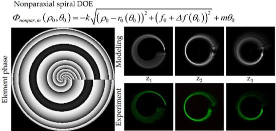
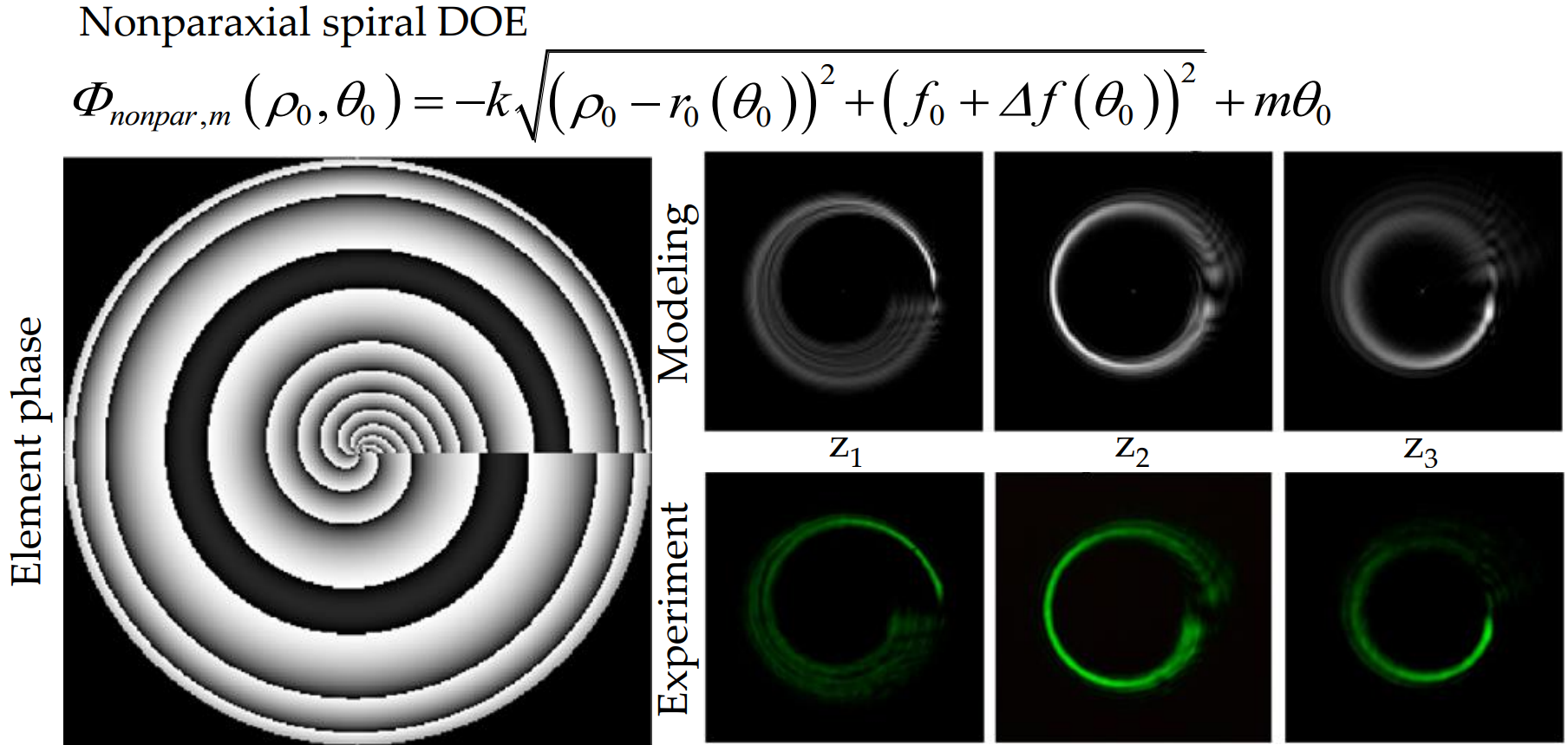
4. Designing DOEs to Generate Spiral Caustics

As a rule, all these optical elements were designed and studied in a paraxial approximation. In the meantime, an optical element that implements the eikonal in (27) presupposes the use of a nonparaxial approach.
Expression (27) implies shaping 3D light spirals. Let us analyze the eikonal in more detail, with the spiral longitudinally extended along the optical axis:
Ψ ( ρ 0 , θ 0 ) = ( ρ 0 r 0 ( θ 0 ) ) 2 + ( f 0 + Δ f ( θ 0 ) ) 2 { ( ρ 0 r 0 ( θ 0 ) ) 2 2 f 0 + Δ f ( θ 0 ) + [ Δ f ( θ 0 ) ] 2 2 f 0 } f 0 ,
where Δ f ( θ 0 ) = ( f 1 f 0 ) 2 π θ 0 = α θ 0 .
Obviously, the longitudinal length of the formed spiral is determined by two terms in curly brackets in Equation (50), containing linear and nonlinear dependence on Δ f ( θ 0 ) , and hence on the angle θ 0 .
Neglecting the constant last term, the DOE phase is approximately described as follows:
Φ p a r ( ρ 0 , θ 0 ) = k Ψ ( ρ 0 , θ 0 ) k 2 f 0 { [ ρ 0 r 0 ( θ 0 ) ] 2 + [ Δ f ( θ 0 ) ] 2 } k α θ 0 .
Expression (51) contains terms nonlinearly dependent on the angle (in the braces) and the last term with the linear angular-dependence. The linear dependence on the angle corresponds to the classic optical vortex of the order p = k α which in the general case is a fractional value [43]. The presence of this term is not necessary for the longitudinal distribution of the spiral, the nonlinear term is mainly responsible for this. An analogy can be drawn with ‘perfect optical vortices’ [44] which have a ring intensity distribution of the same radius regardless of the optical vortices present in the beam. However, the change in the value of the vortex singularity can be used to vary the speed of rotation over the ring of trapped particles [45].
The linear part of the angular dependence in an optical element described by Equation (50) corresponds to the classic optical vortex whose order is proportional to the ratio of the longitudinal spiral extent to the incident laser wavelength:
p = k ( f 1 f 0 ) 2 π = ( f 1 f 0 ) λ
Note, the magnitude of the difference ( f 1 f 0 ) may be several thousand wavelengths (which is normally the case in the experiments), so the order of the vortex in (52) will be of the same magnitude. Too high an order of the extra optical vortex may lead to distortion of not only the on-axis but also the off-axis caustic [11]. We also note that if the order of the optical vortex is too high, even ‘perfect optical vortices’ that such elements form cease to be ‘perfect’, with the radius of the intensity ring becoming order-dependent [46]. Besides, in the experimental realization, when an order of the extra optical vortex is too high [47] the limited resolution of the manufacturing technologies or devices used for the generation of the desired vortex light fields (for example, spatial light modulators or digital micromirror devices) lead to distortion of the field.
This challenge can be addressed via introducing a compensating optical vortex. The phase of a paraxial vortex lens, which focuses into different points of a light spiral in different planes, may be given by
Φ p a r , m ( ρ 0 , θ 0 ) = k ( ρ 0 r 0 ( θ 0 ) ) 2 2 f 0 k Δ f ( θ 0 ) k [ Δ f ( θ 0 ) ] 2 2 f 0 + m θ 0
Equation (53) suggests that if m = ( f 1 f 0 ) / λ , the optical element is structurally simplified:
Φ p a r , m ( ρ 0 , θ 0 ) = k 2 f 0 { [ ρ 0 r 0 ( θ 0 ) ] 2 + [ Δ f ( θ 0 ) ] 2 }
Note, despite the compensation of the linear angular dependence, the nonlinear angular dependence, which is responsible for the longitudinal extension of the spiral, remains.
It stands to reason that the corresponding optical vortex may also be imbedded into the nonparaxial spiral DOE in Equation (50):
Φ n o n p a r , m ( ρ 0 , θ 0 ) = k ( ρ 0 r 0 ( θ 0 ) ) 2 + ( f 0 + Δ f ( θ 0 ) ) 2 + m θ 0
Thus, the technique of shaping a 3D light spiral that uses an optical element implemented through the angular dependence of Equation (37) leads to the generation of both linear and non-linear optical vortices. Linear part of the angular dependence can be varied (both decrease or increase) by introducing an additional vortex phase into the optical element. This provides an extra degree of freedom in variations of the angular momentum of the field and in possible applications.

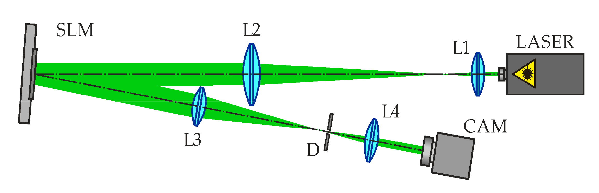
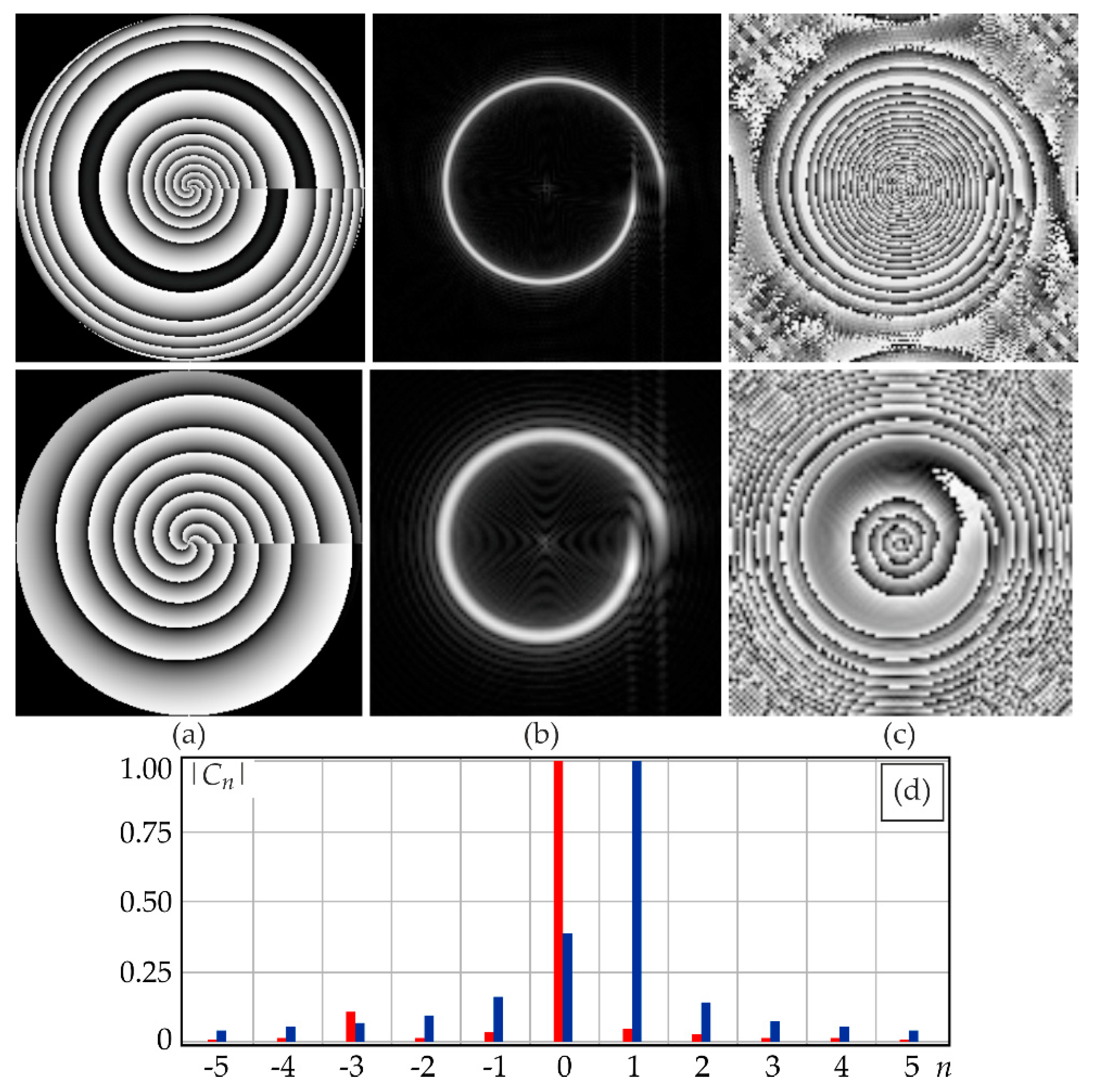
5. Results of the Numerical Simulation and the Experiment

Numerical modeling was conducted using a variety of propagation operators, including the asymptotic operators (39) and (40) derived herein and, by way of verification thereof, through the straightforward numerical integration of the vector Kirchhoff integrals (30), (31). Focusing into a plane spiral curve was numerically simulated using Equations (27), (36), (37) for the following parameters: f 1 = f 0 = 100 mm, m = 0, radiation wavelength 532 nm, while the rest of the parameters—including the DOE radius R d —were varied.
In the experiments, the proposed DOEs were optically implemented using a spatial light modulator (SLM) HOLOEYE PLUTO VIS. An experimental optical setup is shown in Figure 1. An incident linearly polarized Gaussian beam was expanded using a set of lenses L1 and L2 and then directed onto the SLM display. The reflected beam was phase-modulated and spatially filtered using a set of lenses L3, L4, and a pupil D. A video-camera mounted on an optical bench recorded intensity distributions at different distances from the DOE plane. To obtain circularly polarized laser beams, an additional quarter-wave plate put behind lens L4 was utilized in some experiments.
Results of the numerical simulation based on Equations (30) and (31) for the linear x-polarization (meaning that the y-component is zero) and the experiment are shown in Table 1. The inner and outer radii of the spiral were chosen to be r 0 = 1   mm , r 1 = 1.25   mm , and the DOE radius was varied: R d = 1.5 mm (upper row), R d = 0.7 mm (bottom row).
As can be seen (the first column in Table 1), the phase structure of the optical element has a spiral topology similar to the structures considered in [18,24]. It should be noted that the presence of a spiral structure in an optical element, which can be realized also by arrays of metallic nanoparticles [48,49], leads to the appearance of the angular momentum. In contrast to the classical vortex phase singularity, which ensures the formation of the orbital angular momentum (OAM) of the integer order (there is only one angular harmonic) [25,26], the spiral structure leads to the appearance of a set or a sequence of angular harmonics [24,48].
The angular harmonics spectrum can be used to estimate the OAM of a light field [50]:
μ = ( n = n | c n | 2 ) / ( n = | c n | 2 )
where c n are expansion coefficients of the analyzed field E ( r , φ ) by the angular harmonics exp ( i n φ ) :
c n = 1 2 π 0 0 2 π E ( r , φ ) exp ( i n φ ) r d r d φ
In practice, the finite version of expression (56) is often used, as well as the OAM estimation by three arbitrary [51] or two maximum [52] coefficients (57). In addition, due to the conservation of the OAM value during propagation in free space [50], it is convenient to calculate it in the input plane, where the field is spatially bounded, and the integral in (57) has a finite radius limit.
Note that a total angular momentum [53], in addition to the OAM, can have a spin angular momentum (SAM) related with the polarization state of a field [54]. Moreover, in various situations, spin-to-orbit angular momentum conversion can occur [55,56,57,58]. However, here we consider only the OAM associated with the phase structure of the beams.
Figure 2 shows in more detail the x-components of the fields presented in Table 1 and the normalized moduli of the expansion coefficients | c n | of the input fields. As can be seen, in the first case (the first line in Figure 2) the phase practically does not change along the formed light spiral and the OAM is close to zero (μ = −0.03), and in the second case (the second line in Figure 2) there is a vortex phase singularity along the light spiral and the OAM is close to unity (μ = 0.81).
Thus, even for plane/flat curves, the proposed method of the light spiral formation makes it possible to vary the OAM of the light field just by changing the limiting aperture.
From the results given in Table 1, the DOE parameters and the polarization state are seen to have an essential effect on the intensity distribution of the longitudinal E-field component (the second column in Table 1). The polarization state is linked with the emergence of a zero intensity along a line perpendicular to the polarization plane. In the case under study, the linear x-polarization leads to the zero-intensity line along the Y-axis.
Another interesting effect observed in the intensity pattern of the longitudinal E-field component | E z ( u , v ) | 2 is splitting of the spiral curve. This effect is caused by the presence of difference multipliers in the Kirchhoff integral: ( ρ cos θ ρ 0 cos θ s ) and ( ρ sin θ ρ 0 sin θ s ) . These multipliers become zero if the dimensions of an optical element are close to those of the light spiral generated (cf. lines 1 and 2 of Table 1).
For the optical element in row 1 of Table 1, one can clearly see a spiral-shaped zero-phase line. In this region, the rays pass through the optical element without refraction and in parallel with the optical axis. Thus, in this region, the transverse coordinates of output and input points of the rays are the same, meaning that the difference multipliers are zeroed. Rays from other parts are redirected onto the focal curve at some angles. For the optical element in row 2 of Table 1, all its regions direct radiation to a light spiral at some angles to the optical axis. A comparison of the results in Table 1 shows that an increase in the DOE radius leads to a widened curve thickness. Besides, if the DOE radius is smaller than that of the curve under shaping, the light spiral shaped is increased in scale (see the last column).
Computations based on the straightforward numerical integration of the vector Kirchhoff integrals (30), (31) are essentially time-consuming. This has prompted the use of diverse algorithms for accelerating the computing procedures [59,60]. The asymptotic relationships in Equations (39)–(40) we proposed herein enable the number of computing procedures to be decreased due to reducing the 2D integrals to the 1D ones. Importantly, the asymptotic approximation has little or no effect on the computation accuracy. A comparison of modeling results when focusing into a single-turn plane spiral curve obtained through the straightforward integration of Equations (30) and (31) and the asymptotic relationships (39)–(40) for the circularly polarized incident light are depicted in Table 2.
Although the asymptotic approach implies one-dimensional integration, additional computation of the stationary point is required (38). Nevertheless, the number of operations to obtain the final result is less than with double integration (30)–(31). This is because the solution of Equation (38) for each subsequent point uses the solution for the previous point. For the considered examples (Table 2), the calculation time when using the asymptotic approach was on average 1.5 times less than with double direct integration in the case of software implementation in Matlab (R2014a) on a personal computer using a processor Intel (R) Core (TM) i5-3570K CPU @ 3.4 GHz.
From (36), the spiral radius is seen to linearly increase from r 0 to r 1 with increasing angle θ 0 from 0 to 2π. Obviously, the variation can easily be made non-linear. Increasing the number of spiral turns is more challenging. Here, two approaches may be used. With the first, a composite DOE is synthesized [61], with its various parts contributing to different turns of the spiral. The second approach relies on superposition (summation) of complex transmission functions of DOEs that form different turns of the spiral [14,62]. Benefits and drawbacks of the both methods are clearly seen from Table 3, which presents the modeling and experimental results for focusing into a two-turn plane spiral curve for circular polarization (intensities of the x and y-components are identical).
For sectored elements (rows 2 and 3 of Table 3), the ratio of sector areas needs to be fitted thoroughly to ensure that the thickness and intensity of different turns is the same. For composite elements (rows 2 and 4 in Table 3), there is no such requirement and the curve lines are thinner because radiation from the entire element contributes to each element of the curve. As a drawback, we should mention interference effects leading to the generation of extra segments in the spiral.
Given the above-described parameters and putting f 1 f 0 = 1   mm , the extra vortex will have a very high order in (52): p = 1   mm / 0.000532   mm 1879 . An experimental implementation of vortices with high-order topological charge is feasible [40] but requires synthesizing a multi-level DOE with over 2000 × 2000 pixels.
The vortex order can be decreased by decreasing the difference f 1 f 0 to several wavelengths. In particular, to get p = 10, we need f 1 f 0 = 0.005   mm , i.e., if f 0 = 100   mm , then f 1 = 100.005   mm (the spiral radius is much greater than its on-axis length). To get a scale-proportionate spiral, we reduce its radius until several microns, then at f 1 f 0 = 10   μ m ÷ 50   μ m , we find that p = 10 ÷ 50 . Modeling and experimental results on focusing light into a 3D microspiral are presented in Table 4.
Let us analyze in more detail the OAM of 3D microspirals. Figure 3 shows the results of varying the OAM for the 3D microspiral with p = −10. The initially formed spiral has a linear vortex component of the order p = −10, which is clearly seen from the phase structure in the focal plane (the first line in Figure 3). However, the OAM is somewhat different from this value (μ = −9.92) because it also includes a non-linear dependence on the angle, which ensures the longitudinal extent of the spiral. When using an additional vortex phase, the value of the OAM can be increased or decreased: at m = −5 (middle line in Figure 3) an increase occurs (μ = −14.92), and when m = 10 (lower line in Figure 3) we can see almost complete compensation (μ = 0.08). The residual value of the OAM corresponds to the non-linear part that provides the 3D character of the spiral. We suppose this value is related to the ratio of the spiral gap to the average spiral radius.
The spiral length (a distance over which the spiral remains ‘unblurred’ and sharp) is clearly seen to increase with increasing f 1 f 0 . In this case, the optical vortex order p, Equation (52), grows proportionally, as is evident from the structure of the optical elements (column 1 of Table 4).
If the vortex order p is too high, the resulting light caustic gets distorted. This effect can be observed in the bottom row of Table 4. In this case, becoming sufficiently high, the vortex component begins to affect the intensity distribution in the light spiral, ‘dispersing’ the light energy from the central part closer to the periphery. In particular, from the bottom row of Table 4, the spiral inner radius is seen to increase, getting close to its outer radius.
In addition, the experimental implementation of the phase with large orders of the vortex using SLM is problematic. The minimum zone size based on 3 pixels per zone for the used SLM is 3 × 8 µm = 24 µm.
To avoid these adverse effects, we use nonparaxial spiral DOEs of Equation (55) with additional compensating vortex phase. Table 5 shows modeling results for such DOEs.
The results in Table 5 clearly show that in the initial plane ( f 0 = 100   mm ), the initial spiral point located on the radius r 0 = 1   mm is brightest, whereas in the planes f 1 it is the final spiral point which is brightest, located at r 1 = 1.25   mm . Although the DOEs have hardly discernible difference between their phases, the extent of the 3D light spiral from the second DOE is twice as large.

6. Conclusions

In this work, we have deduced asymptotic representations of diffraction integrals that describe behavior of vector electromagnetic fields in the neighborhood of caustics from spiral DOEs.
The distribution of the electric and magnetic fields on a curved surface needs to be known when calculating light forces exerted on a free-form convex conducting microparticle. Besides, when solving a problem of diffraction by a solid (a ball, a cylinder, etc.) bounded by a curved surface, the tangential components of the electromagnetic field need to be joined. The relationships deduced herein can be used for calculating the Poynting vector when evaluating forces exerted on a microparticle trapped in an optical field.
Equations for calculating stationary points and asymptotic relationships that describe components of the electromagnetic field as 1D integrals over a radial variable have been deduced. Without the use of an asymptotic approach, the Kirchhoff integral cannot be reduced to a 1D integral even if both the incident field and the DOE are radially symmetric. One-dimensional asymptotic integrals that describe a vortex DOE to focus into a 3D light spiral have been derived.
The special DOE structure proposed herein because of angular dependence leads to the emergence of the angular momentum of the field. The possibility of the OAM variations due to an additional vortex phase is shown. This provides an extra degree of freedom in controlling the motion of the trapped particle along a 3D spiral curve.

Author Contributions

Conceptualization, V.A.S.; Data curation, S.N.K.; Formal analysis, S.I.K.; Investigation, S.N.K.; Methodology, A.P.P.; Software, Y.S.S. All authors have read and agreed to the published version of the manuscript.

Funding

RF Ministry of Science and Higher Education (007-GZ/Ch3363/26); Russian Foundation for Basic Research (18-58-14001).

Conflicts of Interest

The authors declare that there are no conflict of interest related to this article.

References

  1. Kravtsov, Y.A.; Orlov, Y.I. Geometrical Optics of Inhomogeneous Media; Springer: Berlin/Heidelberg, Germany, 1990; ISBN 978-3-642-84033-3. [Google Scholar]
  2. Born, M.; Wolf, E. Principles of Optics. Electromagnetic Theory of Propagation, Interference and Diffraction of Light, 6th ed.; Pergamon Press: Oxford, UK, 1980; ISBN 0-08-026482-4. [Google Scholar]
  3. Arnol’d, V.I. Singularities of smooth mappings. Russ. Math. Surv. 1968, 23, 1–43. (In Russian) [Google Scholar] [CrossRef]
  4. Poston, T.; Stewart, I. Catastrophe Theory and Its Applications; Dover Publication, Inc.: Mineola, NY, USA, 1978; ISBN 0-486-69271-X. [Google Scholar]
  5. Gilmore, R. Catastrophe Theory for Scientists and Engineers; Dover: New York, NY, USA, 1993; ISBN 978-0-486-67539-8. [Google Scholar]
  6. Babich, V.M.; Buldyrev, V.S. Asymptotic Methods for Short Wave Diffraction Problems; Nauka Publisher: Moscow, Russia, 1972. (In Russian) [Google Scholar]
  7. James, G.L. Geometrical Theory of Diffraction for Electromagnetic Waves, 3rd ed.; Peter Peregrinus Ltd.: London, UK, 1986; ISBN 978-0-86341-062-8. [Google Scholar]
  8. Vainberg, B.R. Asymptotic Methods in Equations of Mathematical Physics; Gordon and Breach Science Publishers: New York, NY, USA, 1989; ISBN 2-88124-664-8. [Google Scholar]
  9. Maslov, V.P. Perturbation Theory and Asymptotic Methods; MGU Publisher: Moscow, Russia, 1965. (In Russian) [Google Scholar]
  10. Maslov, V.P. Operator Methods; Nauka Publisher: Moscow, Russia, 1973. (In Russian) [Google Scholar]
  11. Soifer, V.A.; Kharitonov, S.I.; Khonina, S.N.; Volotovsky, S.G. Caustics of vortex optical beams. Dokl. Phys. 2019, 64, 276–279. [Google Scholar] [CrossRef]
  12. Abramochkin, E.G.; Volostnikov, V.G. Spiral-type beams: Optical and quantum aspects. Opt. Commun. 1996, 125, 302–323. [Google Scholar] [CrossRef]
  13. Abramochkin, E.G.; Volostnikov, V.G. Spiral light beams. Phys. Usp. 2004, 47, 1177–1203. [Google Scholar] [CrossRef]
  14. Khonina, S.N.; Koltyar, V.V.; Soifer, V.A. Techniques for encoding composite diffractive optical elements. Proc. SPIE 2003, 5036, 493–498. [Google Scholar] [CrossRef]
  15. Kotlyar, V.V.; Khonina, S.N.; Soifer, V.A. Iterative calculation of diffractive optical elements focusing into a three dimensional domain and the surface of the body of rotation. J. Mod. Opt. 1996, 43, 1509–1524. [Google Scholar] [CrossRef]
  16. Rodrigo, J.A.; Alieva, T.; Abramochkin, E.; Castro, I. Shaping of light beams along curves in three dimensions. Opt. Express 2013, 21, 20544–20555. [Google Scholar] [CrossRef] [Green Version]
  17. Rodrigo, J.A.; Alieva, T. Polymorphic beams and nature inspired circuits for optical current. Sci. Rep. 2016, 6, 35341. [Google Scholar] [CrossRef] [Green Version]
  18. Alonzo, C.A.; Rodrigo, P.J.; Glückstad, J. Helico-conical optical beams: A product of helical and conical phase fronts. Opt. Express 2005, 13, 1749–1760. [Google Scholar] [CrossRef] [Green Version]
  19. Yang, D.; Li, Y.; Deng, D.; Chen, Q.; Zhang, Y.; Liu, Y.; Gao, J.; Sun, M. Chiral optical field generated by an annular subzone vortex phase plate. Opt. Lett. 2018, 43, 4594–4597. [Google Scholar] [CrossRef]
  20. Degtyarev, S.A.; Porfirev, A.P.; Khonina, S.N. Photonic nanohelix generated by a binary spiral axicon. Appl. Opt. 2016, 55, B44–B48. [Google Scholar] [CrossRef] [PubMed]
  21. Khonina, S.N.; Krasnov, S.V.; Ustinov, A.V.; Degtyarev, S.A.; Porfirev, A.P.; Kuchmizhak, A.; Kudryashov, S.I. Refractive twisted microaxicons. Opt. Lett. 2020, 45, 1334–1337. [Google Scholar] [CrossRef]
  22. Luo, W.; Cheng, S.; Yuan, Z.; Tao, S. Power-exponent-phase vortices for manipulating particles. Acta Opt. Sin. 2014, 34, 93–97. [Google Scholar] [CrossRef]
  23. Lao, G.; Zhang, Z.; Zhao, D. Propagation of the power-exponent-phase vortex beam in paraxial ABCD system. Opt. Express 2016, 24, 18082. [Google Scholar] [CrossRef] [PubMed]
  24. Khonina, S.N.; Ustinov, A.V.; Logachev, V.I.; Porfirev, A.P. Properties of vortex light fields generated by generalized spiral phase plates. Phys. Rev. A 2020, 101, 043829. [Google Scholar] [CrossRef]
  25. Grier, D.G. A revolution in optical manipulation. Nature 2003, 424, 810–816. [Google Scholar] [CrossRef]
  26. Soifer, V.A.; Kotlyar, V.V.; Khonina, S.N. Optical microparticle manipulation: Advances and new possibilities created by diffractive optics. Phys. Part. Nucl. 2004, 35, 733–766. [Google Scholar]
  27. Dholakia, K.; Cizmar, T. Shaping the future of manipulation. Nat. Photonics 2011, 5, 335–342. [Google Scholar] [CrossRef]
  28. Litchinitser, N.M. Structured light meets structured matter. Science 2012, 337, 1054–1055. [Google Scholar] [CrossRef]
  29. Rodrigo, J.A.; Alieva, T. Freestyle 3D laser traps: Tools for studying light-driven particle dynamics and beyond. Optica 2015, 2, 812–815. [Google Scholar] [CrossRef]
  30. Rubinsztein-Dunlop, H.; Forbes, A.; Berry, M.; Dennis, M.; Andrews, D.L.; Mansuripur, M.; Denz, C.; Alpmann, C.; Banzer, P.; Bauer, T.; et al. Roadmap on structured light. J. Opt. 2017, 19, 013001. [Google Scholar] [CrossRef]
  31. Shen, Y.; Wang, X.; Xie, Z.; Min, C.; Fu, X.; Liu, Q.; Gong, M.; Yuan, X. Optical vortices 30 years on: OAM manipulation from topological charge to multiple singularities. Light Sci. Appl. 2018, 8, 90. [Google Scholar] [CrossRef] [PubMed] [Green Version]
  32. Khonina, S.N.; Kazanskiy, N.L.; Karpeev, S.V.; Butt, M.A. Bessel beam: Significance and applications—A progressive review. Micromachines 2020, 11, 997. [Google Scholar] [CrossRef] [PubMed]
  33. Brebbia, C.A. The Boundary Element Method for Engineers, 2nd ed.; Pentech Press: London, UK, 1980; ISBN 978-0727302052. [Google Scholar]
  34. Barton, J.P. Electromagnetic field calculations for an irregularly shaped, nearspheroidal particle with arbitrary illumination. J. Opt. Soc. Am. 2002, 19, 2429–2435. [Google Scholar] [CrossRef] [PubMed]
  35. Soifer, V.A. (Ed.) Methods for Computer Design of Diffractive Optical Elements; John Willey and Sons: New York, NY, USA, 2002; ISBN 978-0-471-09533-0. [Google Scholar]
  36. Zhang, K.; Li, D. Electromagnetic Theory for Microwaves and Optoelectronics; Springer Science & Business Media: Berlin, Germany, 2007; ISBN 978-3-540-74295-1. [Google Scholar]
  37. Peng, Z.; Lim, K.; Lee, J. A boundary integral equation domain decomposition method for electromagnetic scattering from large and deep cavities. J. Comput. Phys. 2015, 280, 626–642. [Google Scholar] [CrossRef]
  38. Syubaev, S.; Zhizhchenko, A.; Vitrik, O.; Porfirev, A.; Fomchenkov, S.; Khonina, S.; Kudryashov, S.; Kuchmizhak, A. Chirality of laser-printed plasmonic nanoneedles tunable by tailoring spiral shape pulses. Appl. Surf. Sci. 2019, 470, 526–534. [Google Scholar] [CrossRef]
  39. Soskin, M.S.; Vasnetsov, M.V. Singular optics. Prog. Opt. 2001, 42, 219–276. [Google Scholar] [CrossRef]
  40. Dennis, M.R.; O’Holleran, K.; Padgett, M.J. Singular optics: Optical vortices and polarization singularities. Prog. Opt. 2009, 53, 293–364. [Google Scholar] [CrossRef]
  41. Kharitonov, S.I.; Volotovsky, S.G.; Khonina, S.N.; Kazanskiy, N.L. Diffraction catastrophes and asymptotic analysis of caustics from axisymmetric optical elements. Proc. SPIE 2019, 11146, 111460K. [Google Scholar] [CrossRef]
  42. Golub, M.A.; Kazanskiy, N.L.; Sisakyan, I.N.; Soifer, V.A.; Kharitonov, S.I. Diffraction calculation for an optical element which focuses into a ring. Optoelectron. Instrum. Data Process. 1987, 23, 7–14. [Google Scholar]
  43. Berry, M.V. Optical vortices evolving from helicoidal integer and fractional phase steps. J. Opt. A 2004, 6, 259–268. [Google Scholar] [CrossRef]
  44. Ostrovsky, A.S.; Rickenstorff-Parrao, C.; Arrizón, V. Generation of the “perfect” optical vortex using a liquid-crystal spatial light modulator. Opt. Lett. 2013, 38, 534–536. [Google Scholar] [CrossRef]
  45. Chen, M.; Mazilu, M.; Arita, Y.; Wright, E.M.; Dholakia, K. Dynamics of micro particles trapped in a perfect vortex beam. Opt. Lett. 2013, 38, 4919–4922. [Google Scholar] [CrossRef] [PubMed]
  46. Pinnell, J.; Rodríguez-Fajardo, V.; Forbes, A. How perfect are perfect vortex beams? Opt. Lett. 2019, 44, 5614–5617. [Google Scholar] [CrossRef] [PubMed]
  47. Qiao, Z.; Xie, G.; Wu, Y.; Yuan, P.; Ma, J.; Qian, L.; Fan, D. Generating high-charge optical vortices directly from laser up to 288th order. Laser Photonics Rev. 2018, 12, 1800019. [Google Scholar] [CrossRef] [Green Version]
  48. Lawrence, N.; Trevino, J.; Negro, L.D. Control of optical orbital angular momentum by Vogel spiral arrays of metallic nanoparticles. Opt. Lett. 2012, 37, 5076–5078. [Google Scholar] [CrossRef]
  49. Negro, L.D.; Wang, R.; Pinheiro, F.A. Structural and spectral properties of deterministic aperiodic optical structures. Crystals 2016, 6, 161. [Google Scholar] [CrossRef] [Green Version]
  50. Khonina, S.N.; Kotlyar, V.V.; Soifer, V.A.; Pääkkönen, P.; Simonen, J.; Turunen, J. An analysis of the angular momentum of a light field in terms of angular harmonics. J. Mod. Opt. 2001, 48, 1543–1557. [Google Scholar] [CrossRef]
  51. Ni, B.; Guo, L.; Yue, C.; Tang, Z. A novel measuring method for arbitrary optical vortex by three spiral spectra. Phys. Lett. A 2017, 381, 817–820. [Google Scholar] [CrossRef]
  52. Khonina, S.N.; Podlipnov, V.V.; Karpeev, S.V.; Ustinov, A.V.; Volotovsky, S.G.; Ganchevskaya, S.V. Spectral control of the orbital angular momentum of a laser beam based on 3D properties of spiral phase plates fabricated for an infrared wavelength. Opt. Express 2020, 28, 18407–18417. [Google Scholar] [CrossRef]
  53. Bliokh, K.Y.; Alonso, M.A.; Ostrovskaya, E.A.; Aiello, A. Angular momenta and spin–orbit interaction of non-paraxial light in free space. Phys. Rev. A 2010, 82, 063825. [Google Scholar] [CrossRef] [Green Version]
  54. Angelsky, O.V.; Bekshaev, A.Y.; Maksimyak, P.P.; Maksimyak, A.P.; Mokhun, I.I.; Hanson, S.G.; Zenkova, C.Y.; Tyurin, A.V. Circular motion of particles suspended in a Gaussian beam with circular polarization validates the spin part of the internal energy flow. Opt. Express 2012, 20, 11351–11356. [Google Scholar] [CrossRef] [PubMed] [Green Version]
  55. Marrucci, L.; Manzo, C.; Paparo, D. Optical spin-to-orbital angular momentum conversion in inhomogeneous anisotropic media. Phys. Rev. Lett. 2006, 96, 163905. [Google Scholar] [CrossRef] [PubMed] [Green Version]
  56. Zhao, Y.; Edgar, J.S.; Jeffries, G.D.M.; McGloin, D.; Chiu, D.T. Spin-to-orbital angular momentum conversion in a strongly focused optical beam. Phys. Rev. Lett. 2007, 99, 073901. [Google Scholar] [CrossRef] [PubMed]
  57. Bliokh, K.Y.; Rodriguez-Fortuno, F.; Nori, F.; Zayats, A.V. Spin-orbit interactions of light. Nat. Photonics 2015, 9, 796–808. [Google Scholar] [CrossRef]
  58. Khonina, S.N.; Karpeev, S.V.; Paranin, V.D.; Morozov, A.A. Polarization conversion under focusing of vortex laser beams along the axis of anisotropic crystals. Phys. Lett. A 2017, 381, 2444–2455. [Google Scholar] [CrossRef]
  59. Balalaev, S.A.; Khonina, S.N. Realisation of fast algorithm of Kirchhoff’s diffraction integral on an example of Bessel modes. Comput. Opt. 2006, 30, 69–73. [Google Scholar]
  60. Khonina, S.N.; Ustinov, A.V.; Kovalyov, A.A.; Volotovsky, S.G. Near-field propagation of vortex beams: Models and computation algorithms. Opt. Mem. Neural Netw. 2014, 23, 50–73. [Google Scholar] [CrossRef]
  61. Golub, M.A.; Doskolovich, L.L.; Kazanskiy, N.L.; Kharitonov, S.I.; Sisakian, I.N.; Soifer, V.A. Focusators at letters diffraction design. Proc SPIE 1991, 1500, 211–221. [Google Scholar] [CrossRef]
  62. Khonina, S.N.; Kotlyar, V.V.; Lushpin, V.V.; Soifer, V.A. A method for design of composite DOEs for the generation of letter image. Opt. Mem. Neural Netw. 1997, 6, 213–220. [Google Scholar]
Figure 1. An optical setup for generating the laser beams under study: LASER—a solid-state laser (λ = 532 nm), L1, L2, L3, and L4—lenses with focal lengths of 25, 150, 500, and 250 mm, respectively, SLM—a spatial light modulator HOLOEYE PLUTO VIS, D—a circular pupil, and CAM—a video-camera.
Photonics 08 00024 g001
Figure 2. x-components of the fields considered in Table 1: (a) phase of the input field, (b) amplitude and (c) phase of the field in the focal plane, (d) normalized moduli of the expansion coefficients | c n | for the input fields in the first line (red) and in the second line (blue).
Photonics 08 00024 g002
Figure 3. Variations of the orbital angular momentum (OAM) for the 3D microspiral with p = −10 by means of an additional vortex phase m = 0 (top line), m = −5 (middle line), m = 10 (bottom line): (a) phase of the input field, (b) amplitude, and (c) phase of the field in the focal plane, (d) normalized moduli of the expansion coefficients | c n | for the input fields in the first (blue), second (green), and third (red) lines.
Photonics 08 00024 g003
Table 1. Numerical modeling and experiment on focusing into a single-turn spiral curve for the linear x-polarization.
Optical Element Phase
λ = 532 nm, f1 = f0 = 100 mm,
r0 = 1 mm, r1 = 1.25 mm
Intensity Distribution, x, y ∈ [−1.5 mm, 1.5 mm]
z = 100 mm
Modeling
|E(u,v)|2
z = 80 mmz = 100 mmz = 120 mm
Rd = 1.5 mm|Ex(u,v)|2modeling
Photonics 08 00024 i001 Photonics 08 00024 i002 Photonics 08 00024 i003 Photonics 08 00024 i004 Photonics 08 00024 i005
|Ez(u,v)|2experimental
Photonics 08 00024 i006 Photonics 08 00024 i007 Photonics 08 00024 i008 Photonics 08 00024 i009
Rd = 0.7 mm|Ex(u,v)|2modeling
Photonics 08 00024 i010 Photonics 08 00024 i011 Photonics 08 00024 i012 Photonics 08 00024 i013 Photonics 08 00024 i014
|Ez(u,v)|2experimental
Photonics 08 00024 i015 Photonics 08 00024 i016 Photonics 08 00024 i017 Photonics 08 00024 i018
Table 2. Comparative modeling of focusing into a single-turn spiral curve: Equations (30)–(31) vs. Equations (39)–(40), for circular polarization.
Calculation Parameters
λ = 532 nm, f1 = f0 = 100 mm
Calculation MethodIntensity Distribution of the Electric Field Components in the Plane z = 100 mm
|Ex(u,v)|2|Ez(u,v)|2
Input field: Rd = 1.5 mm
Photonics 08 00024 i019
Output field:
r0 = 1 mm, r1 = 1.25 mm,
x, y ∈ [−1.5 mm, 1.5 mm]
Direct
integration
(30)–(31)
Photonics 08 00024 i020 Photonics 08 00024 i021
Asymptotic
(39)–(40)
Photonics 08 00024 i022 Photonics 08 00024 i023
Input field: Rd = 1.0 mm
Photonics 08 00024 i024
Output field:
r0 = 2 mm, r1 = 2.5 mm,
x, y ∈ [−3 mm, 3 mm]
Direct
integration
(30)–(31)
Photonics 08 00024 i025 Photonics 08 00024 i026
Asymptotic
(39)–(40)
Photonics 08 00024 i027 Photonics 08 00024 i028
Table 3. Focusing into a two-turn spiral of circularly polarized light: modeling vs. experiment.
Parameters
λ = 532 nm,
f1 = f0 = 100 mm
Optical Element PhaseIntensity Distribution of the Electric Field
Components in the Plane z = 100 mm
Modeling
|Ex(u,v)|2
Modeling
|Ez(u,v)|2
Experimental
|E(u,v)|2
Rd = 1.5 mm,
r0 = 1 mm,
r1 = 1.25 mm,
r2 = 1.5 mm
Sectorial
Photonics 08 00024 i029 Photonics 08 00024 i030 Photonics 08 00024 i031 Photonics 08 00024 i032
Compositional
Photonics 08 00024 i033 Photonics 08 00024 i034 Photonics 08 00024 i035 Photonics 08 00024 i036
Rd = 1.5 mm,
r0 = 2 mm,
r1 = 2.5 mm,
r2 = 3 mm
Sectorial
Photonics 08 00024 i037 Photonics 08 00024 i038 Photonics 08 00024 i039 Photonics 08 00024 i040
Compositional
Photonics 08 00024 i041 Photonics 08 00024 i042 Photonics 08 00024 i043 Photonics 08 00024 i044
Table 4. Focusing into a single-turn 3D micro-spiral curve: modeling vs. experiment.
Element Phase
λ = 532 nm, Rd = 120λ,
f0 = 100λ
Distortion of the Total Intensity of the Components
Electric Field in Different Planes (x, y = ∈ [−120λ, 120λ])
z = 100λz = 110λz = 120λz = 130λ
f1 = 100λ, p = 0modeling
Photonics 08 00024 i045 Photonics 08 00024 i046 Photonics 08 00024 i047 Photonics 08 00024 i048 Photonics 08 00024 i049
experimental
Photonics 08 00024 i050 Photonics 08 00024 i051 Photonics 08 00024 i052 Photonics 08 00024 i053
f1 = 110λ, p = −10modeling
Photonics 08 00024 i054 Photonics 08 00024 i055 Photonics 08 00024 i056 Photonics 08 00024 i057 Photonics 08 00024 i058
experimental
Photonics 08 00024 i059 Photonics 08 00024 i060 Photonics 08 00024 i061 Photonics 08 00024 i062
f1 = 120λ, p = −20modeling
Photonics 08 00024 i063 Photonics 08 00024 i064 Photonics 08 00024 i065 Photonics 08 00024 i066 Photonics 08 00024 i067
experimental
Photonics 08 00024 i068 Photonics 08 00024 i069 Photonics 08 00024 i070 Photonics 08 00024 i071
f1 = 150λ, p = −50modeling
Photonics 08 00024 i072 Photonics 08 00024 i073 Photonics 08 00024 i074 Photonics 08 00024 i075 Photonics 08 00024 i076
experimental
Photonics 08 00024 i077 Photonics 08 00024 i078 Photonics 08 00024 i079 Photonics 08 00024 i080
Table 5. Focusing into a single-turn 3D spiral curve: modeling vs. experiment.
Element Phase
λ = 532 nm, Rd = 1.5 mm,
r0 = 1 mm, r1 = 1.25 mm
Distortion of the Total Intensity of the Components
Electric Field in Different Planes (x, y = ∈ [–1.5 mm, 1.5 mm])
z = 100 mmz = 150 mmz = 200 mm
f0 = 100 mm, f1 = 150 mm
Photonics 08 00024 i081
modeling
Photonics 08 00024 i082 Photonics 08 00024 i083 Photonics 08 00024 i084
experimental
Photonics 08 00024 i085 Photonics 08 00024 i086 Photonics 08 00024 i087
f0 = 100 mm, f1 = 200 mm
Photonics 08 00024 i088
modeling
Photonics 08 00024 i089 Photonics 08 00024 i090 Photonics 08 00024 i091
experimental
Photonics 08 00024 i092 Photonics 08 00024 i093 Photonics 08 00024 i094
Publisher’s Note: MDPI stays neutral with regard to jurisdictional claims in published maps and institutional affiliations.

