1. Introduction
The performance of a telescope system is heavily reliant upon the effective aperture of the primary mirror. The universe observations and the detection of remote sensing require optical systems with better performance [
1]; therefore, the requirement for large-aperture telescopes is increasing. The traditional fabrication technology is hardly capable of fabricating a monolithic mirror larger than the 10 m class; to achieve better performance, the most common approach is the segmented mirror plan, wherein the monolithic mirror is replaced by several smaller mirrors. These small mirrors can be combined into a large mirror, avoiding the issues related to fabrication technology. Compared with monolithic mirrors, the equivalent aperture of segmented mirrors can be even greater than 30 m, achieving brilliant performance that monolithic mirrors cannot currently obtain. However, the diffraction effect of large segmented mirrors is more complicated than for monolithic mirrors [
2,
3].
The first large-aperture telescope with a segmented primary mirror in the world was the Keck telescope, built in 1991. The Keck has a 10 m effective aperture combined with 36 small segments, and each segment is 1.8 m large. The success and the great performance of the Keck confirmed the potential of segmented designs. Various countries in the world started to design and build segmented telescopes, such as the Hobby–Eberly Telescope (HET), the South Africa Large Telescope (SALT), Gran Telescopio Canarias (GTC), the European Extremely Large Telescope (E-ELT), and the Thirty Meter Telescope (TMT) [
4,
5,
6]. As the cooperator of the TMT, China is also attaching great importance to segmented telescope technology; the first segmented mirror design in China was LAMOST. Since the James Webb Space Telescope (JWST) started its operation, the importance of segmented mirror technology has been further enhanced, and one of the key problems related to segmented mirrors, the co-phasing of the segments, has become a research priority.
The co-phasing of segmented mirrors adjusts the positions of all of the segments, ensuring that the segments are on the same equiphase surface. The most researched and most sensitive co-phase error is the piston error, which is the position deviation in the direction of the optical axis. Since the appearance of the Keck telescope, the co-phasing problem has been continually researched for decades. In recent years, many valuable co-phasing methods have been researched. Li Yang et al. proposed a piston-measuring method based on hyperspectral images [
7], whereby the measuring precision can reach a few micrometers, and the measurement range can reach about 130 μm. Li Xiao yang et al. proposed a modified Shack–Hartmann (S–H) sensor method [
8]; this research resolved some of the location error problems related to the S–H sensor. Seichi Sato et al. proposed a cross-fringe piston sensor method, achieving a measurement precision of about 15 nm when the piston is smaller than 5 μm [
9]. Yang Lili et al. proposed a piston-measuring method based on vortex phase-shifting interferometry, and the measurement precision can reach 4.04 nm [
10] when the piston is within one wavelength. Zhao weirui et al. proposed a method to measure the piston error by using multiple neural network coordination of feature-enhanced images [
11]; the precision can be expected to achieve a sub-nanometer class, and the measurable range is about 30 μm. However, these pieces of recent research have been concerned with the measurement precision of the piston but not with achieving a large measurable range, with the biggest range amongst them being 130 μm and the smallest being even smaller than 1 μm. For the large segmented mirror, such as the JWST, the measurable range of the piston was designed to be more than 300 μm for the coarse phasing stage, and the precision was designed to be better than
in the fine phasing stage [
12].
Optical interferometry is a measurement method with ultra-high accuracy, which is often used for the measurement of mirror surface shapes and micro-displacement. Its basic principle is to use the intensity distribution of interference fringes to calculate the deviation from the ideal equiphase surface.
However, the problem of piston error in interferometry detection is that the size of the piston often exceeds the detection range of general interferometry. For this problem, the commonly used method is to use dual-wavelength synthesis to expand the measurement range. The principles of the synthetic wavelength method have been described in previous studies [
13]; in this study, we introduced a phase-shifting interference method to measure the piston error and used a variable synthetic wavelength strategy to expand the measurable range to more than 1 mm. However, although the synthetic wavelength method can greatly expand the detection range, it still has a disadvantage, which is that the synthetic wavelength method also expands the influence of the measurement error while expanding the range, resulting in low detection accuracy in a large range. Although the measurement error can be gradually reduced by reducing the synthetic wavelength, this method is still relatively complex in the coarse phasing processes and it takes a long time to measure and adjust.
This study aims to provide a simple system and efficient co-phasing method for the coarse phasing process when the piston is relatively large; for this, a piston error measurement method based on multiwavelength interferometry has been proposed, which we called the multiwavelength wavefront linear fit (MWLF) method. Different from the synthetic wavelength method, this method uses wavefront data at different wavelengths in a continued waveband. Through the comprehensive calculation of multiple sets of data, the influence of the calculation error caused by the wavefront detection error is reduced while maintaining the advantages of interferometry in the measurement range. MWLF is suitable for the rapid convergence experienced in the coarse phasing stage, wherein large piston errors occur.
2. Methodology
2.1. Principle of the MWLF
Assume that there is a piston error between two segments and the size of the piston is
P; then, use a wavelength of
to achieve the interference fringe and calculate the wavefront. The principle of the phase-shifting interference method to measure the wavefront data was introduced in our previous study [
13]. Due to periodic wrapping, the original optical path difference between the two sub-mirrors was limited in
; assuming that the system is exposed to air, the refractive index
n = 1, and the result of the optical path difference caused by the piston has the size of
, under single-wavelength interference, the solution wavefront is as follows:
where
is the optical path difference, which is defined as the difference between two segments.
P is the piston error, and [] is the round function since the wavefront data will be wrapped.
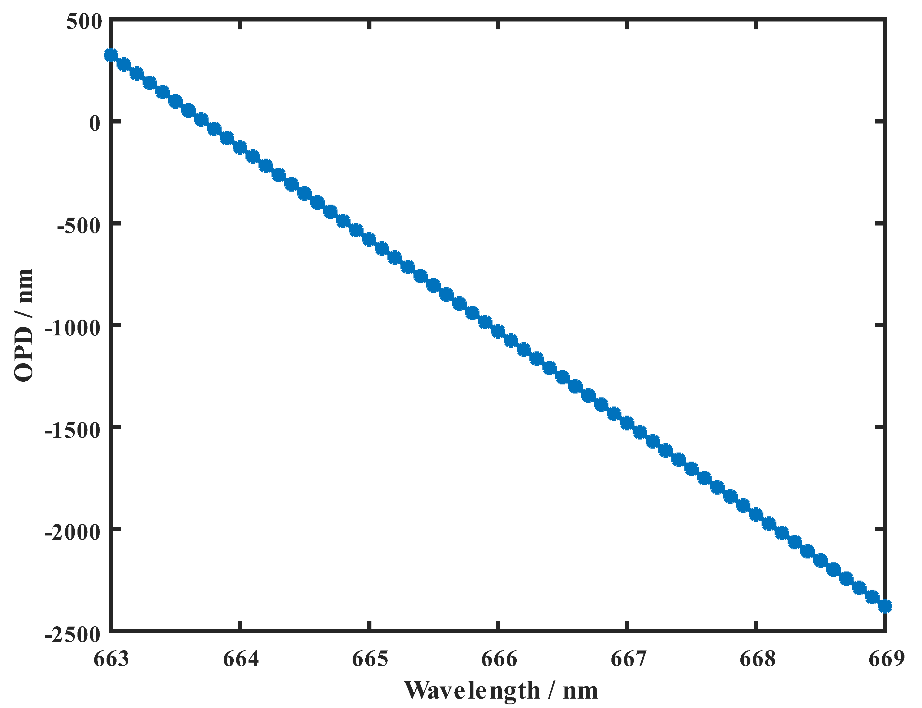
If different wavelengths in one continuous waveband are taken for measurement and calculation for a fixed piston, the results shown in
Figure 1 can be obtained. The ordinate in the figure is the optical path difference,
OPD, between the different segments, and the abscissa is the measured wavelength.
As can be seen in
Figure 1, for an equally sized piston error tested under different wavelengths, different optical path differences were calculated, and the size of the
OPD was a linear function within a small waveband. For Equation (1), the existence of some wavebands made the rounding function equal to a constant, and for the linear area shown in
Figure 1, its slope
can be expressed as follows:
Equation (2) indicates that the slope of the linear area can calculate the piston error. Then, the piston information can be calculated by the measured data of the
OPD at different wavelengths. The calculated piston errors can be expressed as follows. The average value of all wavelengths was used to define the calculated piston errors:
where
is the calculated piston error, and
is the calculated slope, which is calculated by the least-squares minimization.
is the number of data, and
is the measured wavelength in the same liner region.
The
in Equation (3) can be calculated by the wavefront data as follows:
where
is the wavefront data of
, and can be measured by the phase-shifting interference method,
and
are the data masks for the two segments, respectively, and
and
are the data numbers in the masks.
2.2. Data Correction of MWLF
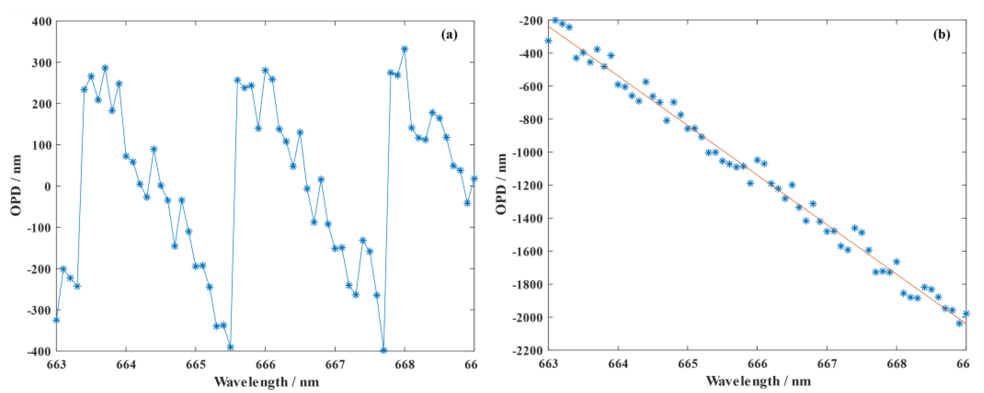
The linear area shown in
Figure 1 tends to be narrow when the piston error is relatively large. In this case, the calculation data of different wavelengths may contain multi-linear areas; therefore, the
OPD result will be wrapped.
In this case, there are two solutions for measuring the large piston error. The first is to reduce the sampling interval between the wavelengths so that all of the data can still be in the same linear area. However, this plan needs to predict the approximate size of the existing piston in advance, and it requires a tunable laser light source with great performance so that the sampling interval can be small enough. In the second solution, the measurement data between different linear areas need to be compensated and corrected so that they can still be approximately linear to obtain a correct solution result. This is similar to the unwrapping of the wrapped wavefront. The difference is that the unwrapping problem is under the same wavelength, and the period of all of the data is consistent, while for multiwavelength data correction, each piece of wavelength data has different periods, and each piece of data should be compensated for a corresponding period. After the data correction,
Figure 1 can be shown as
Figure 2; it needs to be noted that the
OPD is not strictly linear in
Figure 2 since the slope in different linear areas is not the same, but in most cases it can be assumed to be linear. As shown in Equation (1), the slope difference between adjacent linear areas is 1; for example, for a 100 μm piston, and 663 nm to 669 nm waveband, the slope is 302 to 299 for the four linear areas, respectively. When the piston is 50 μm, there are only two different linear areas in this waveband, and their slope is 121 and 120, respectively. For a smaller piston, the linear area will exist only once in this waveband.
3. Simulation
3.1. Simulation of MWLF Method and Synthetic Wavelength Method
In the case of wavefront interferometry, the final wavefront measurement results will be affected by many factors, such as environmental noise, system noise, vibration, temperature change, and airflow change. These errors will lead to instability in the interference fringe and will change with time. As shown in
Figure 3, the change in the interference fringes is essentially a change in the optical path difference caused by the change in the refractive index and travel. Although the data will often be multiple-sampled and averaged during interference measurements to reduce the influence of errors, the influence on high-precision co-phase measurements is still obvious.
When wavefront measurement errors exist, Equation (1) changes as follows, where
is the error term.
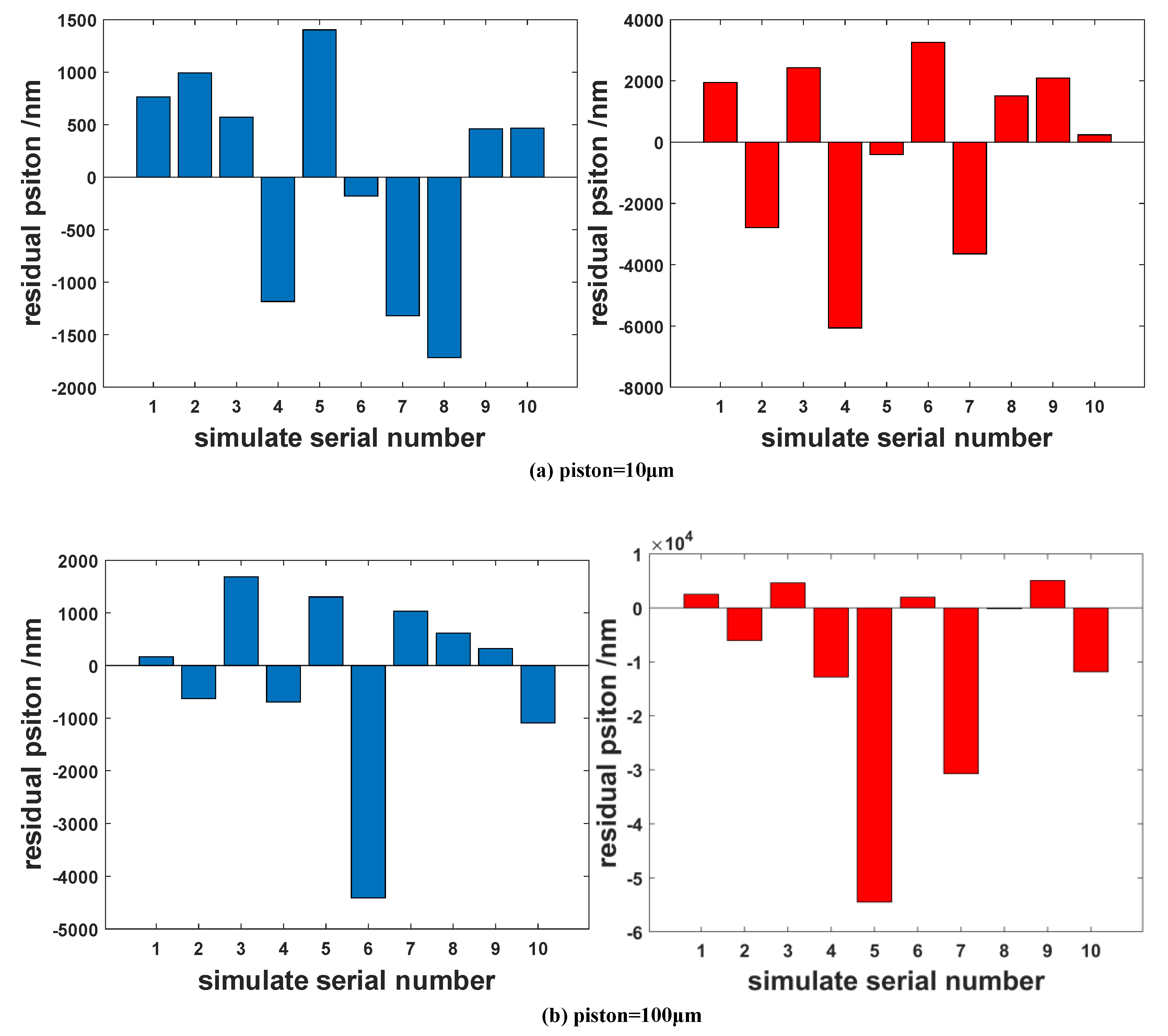
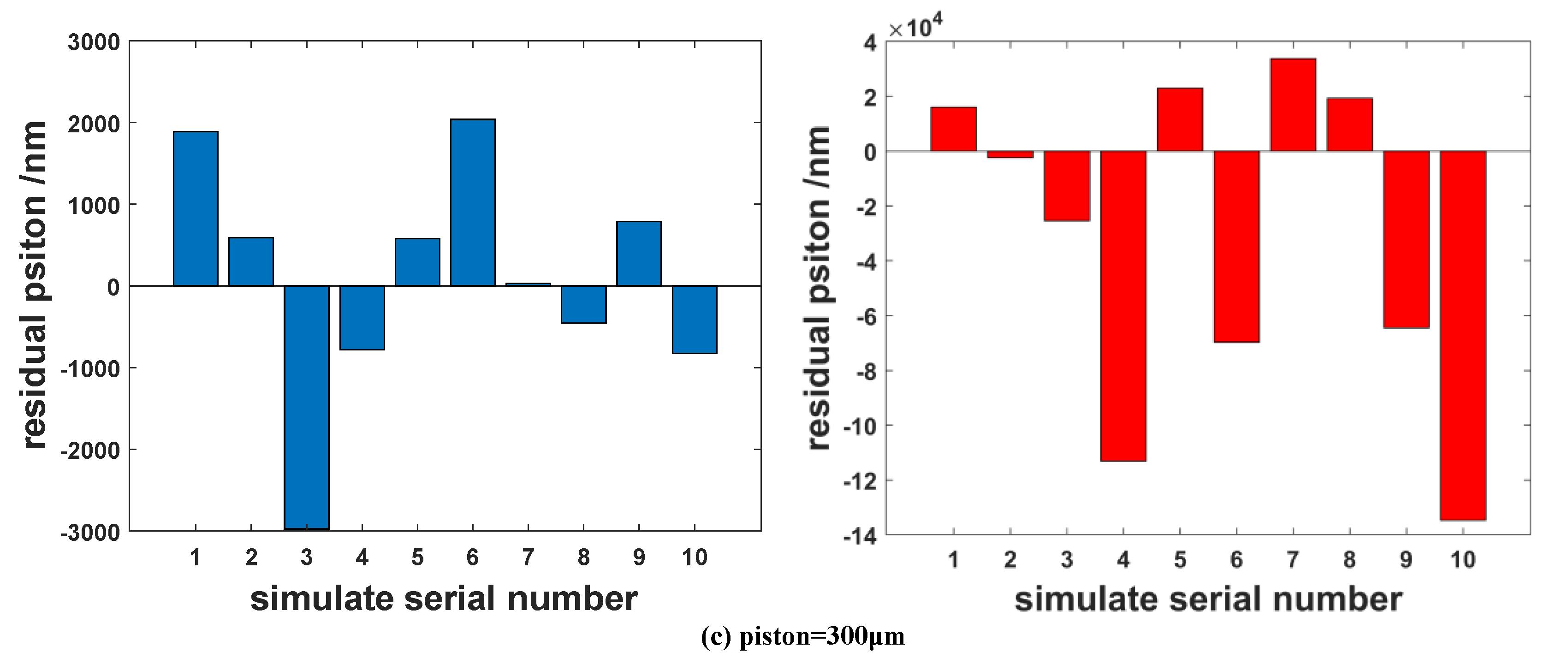
The numerical simulation assumes a relatively large error of
with a random distribution. The sizes of the piston errors are assumed to be 10 μm, 100 μm, and 300 μm, respectively. The traditional dual-wavelength interference method and the MWLF method are both simulated using the same data and with the same distribution of
. The simulation results are shown in
Figure 4. The blue histogram on the left is the simulation results of the MWLF method, the red histogram on the right is the simulation results of the dual-wavelength interference method, the ordinate is the residual piston between the measured value and the input value, and the abscissa is the Nth simulation result.
For the MWLF method, with reference to the experimental equipment, 61 sets of wavefront data with a 0.1 nm sample interval in the waveband of 663 nm to 669 nm were used for the simulation. For the dual-wavelength interference method, the selected test wavelengths were 663 nm/669 nm (the measurement range was about 18 μm), 663 nm/664 nm (the measurement range was about 110 μm), and 663 nm/663.3 nm (the measurement range was about 360 μm). The measurement range was slightly larger than the selected piston to achieve an ideal measurement accuracy. For the two methods, each input piston was simulated ten times.
For a 10 μm piston input, as shown in
Figure 4a, the simulation’s piston residual RMS of the MWLF method is 1.07 μm, and the simulation’s piston residual RMS of the synthetic wavelength method is 3.07 μm. For a 100 μm piston input, as shown in
Figure 4b, the simulation’s piston residual RMS of the MWLF method is 1.74 μm, and the simulation piston’s residual RMS of the synthetic wavelength method is 19.1 μm. For a 300 μm piston input, as shown in
Figure 4c, the simulation’s piston residual RMS of the MWLF method is 1.46 μm, and the simulation’s piston residual RMS of the synthetic wavelength method is 60.3 μm. The simulation’s results indicate that for the synthetic wavelength method, the influence of the measurement error will be proportionally amplified with an increased measurement range. In the previous study [
13], we proposed a multiwavelength phase-shifting interferometry method based on multiple groups of different synthetic wavelengths. By flexibly switching the size of the synthetic wavelength, the measured piston can be gradually reduced, and finally, convergence is achieved, that is, from a coarse phasing process to a fine phasing process. However, this method is a complicated process, requiring multiple adjustments to select the appropriate synthetic wavelength for repeated measurements, and the convergence speed is slow. However, for the MWLF method, the measurement process is relatively simple and rapid since MWLF can maintain better measurement precision for a large piston.
3.2. Error Analysis and Discussion
For the MWLF method, the simulation results show that the measurements of a large piston do not cause a significant decrease in measurement precision, which is basically maintained at 1.5 μm, and the measurement range of the MWLF method only depends on the sample interval of the wavelength and the wavefront measure error of
. For the simulation conditions of
Figure 4 (0.1 nm for the wavelength sample interval and
for the wavefront error), the maximum measurable range can reach about 500 μm. In the ideal case of no wavefront error, it can reach about 1000 μm. Therefore, it can be considered that the MWLF method is a more suitable piston measurement method in the coarse phase process of segmented mirrors, helping the segments to reduce piston errors rapidly. Normally, it is required that the piston errors are less than half of the measured wavelength to make sure that the coarse phasing process can be considered as successfully entering the fine phasing process. Using the commonly used He-Ne laser as an example, the coarse phase detection accuracy is required to be within 316.4 nm. For the MWLF method, from the simulation results, when the wavelength sample interval is increased to 0.01 nm or the wavefront error is reduced to
, the detection accuracy can be better than 300 nm RMS. The influence of the wavelength sample interval and the wavefront measurement error on the range and detection accuracy of a piston error are shown in
Table 1, as follows.
4. Experiment
4.1. Experimental Setup
The experimental system used in this study was a spherical 400 mm aperture segmented mirror system that combined three segments. However, since the co-phase detection between the two segments and between the multiple segments are not different in theory, for the sake of decreasing the system complexity, only two segments were used for the theoretical verification test.
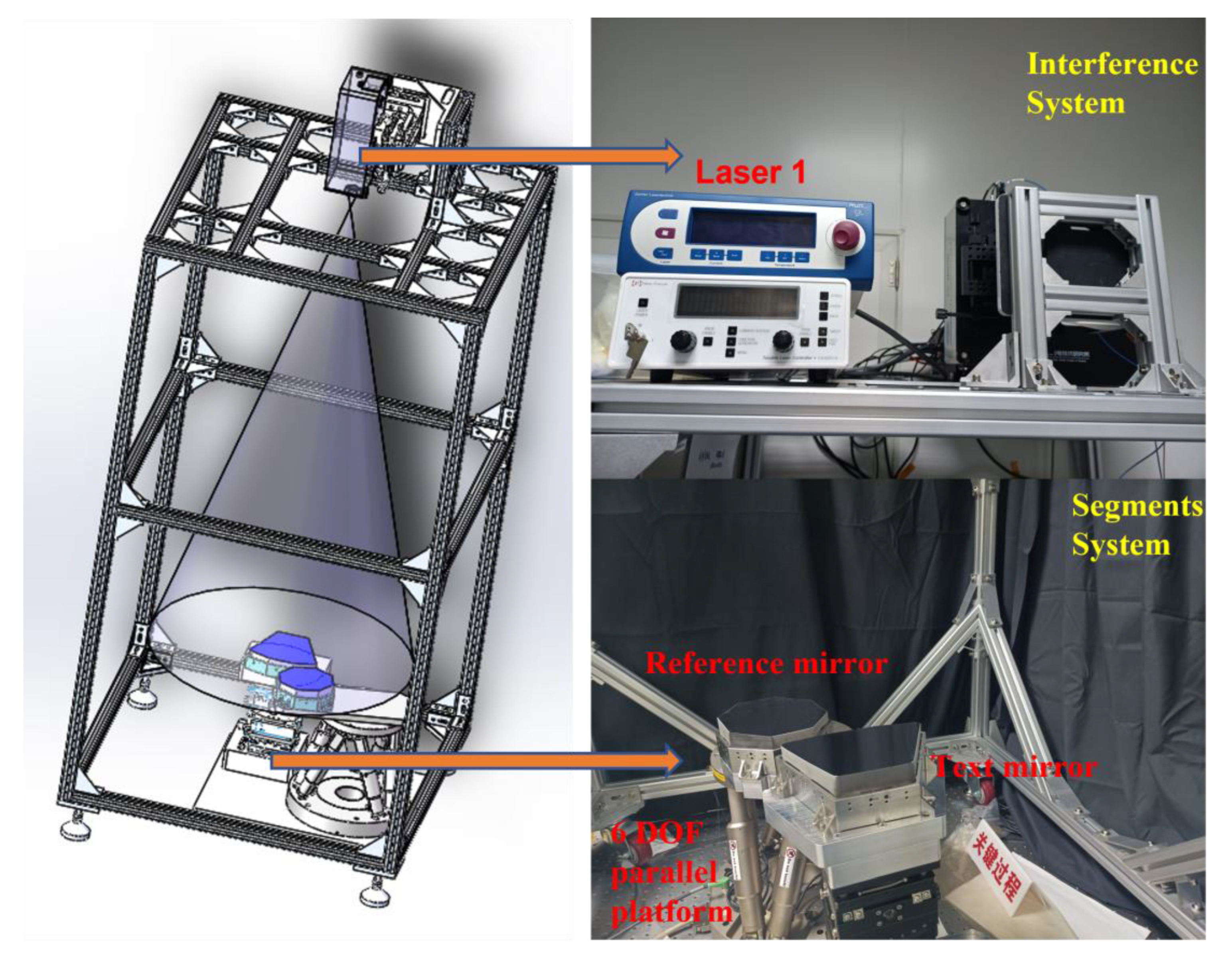
As shown in
Figure 5, the experimental system consisted of an interferometer, a test tower, and two segmented mirrors. The interferometer was a multiwavelength Fizeau interferometer jointly developed by the Institute of Optoelectronic Technology, Chinese Academy of Sciences, and the Shanghai Institute of Technical Physics, Chinese Academy of Sciences. Through the tunable laser light source, the measured wavelength can vary from 650 nm to 680 nm, and the wavelength interval can reach 0.1 nm. The size of the test tower was 2.5 m × 0.9 m × 0.9 m. The measured segments formed a spherical mirror, the effective aperture of each segment was about 150 mm, the material of the mirror was microcrystalline glass, the radius of curvature was 1500 mm, and the mirror’s surface accuracy was better than 1/50
λ RMS. The segment adjustment mechanism was the 6-DOF parallel platform produced by PI Company, and the model number was H-850. This adjustment mechanism had a displacement accuracy of 100 nm. The whole system was located on a high-precision optical isolation platform.
4.2. Measurement Process
To clear the measurement process of the experiment, the detailed introduction of each step is as follows:
Install all experimental equipment and adjust the segmented mirrors to allow the interference fringes of each segment to be obtained by the CCD camera.
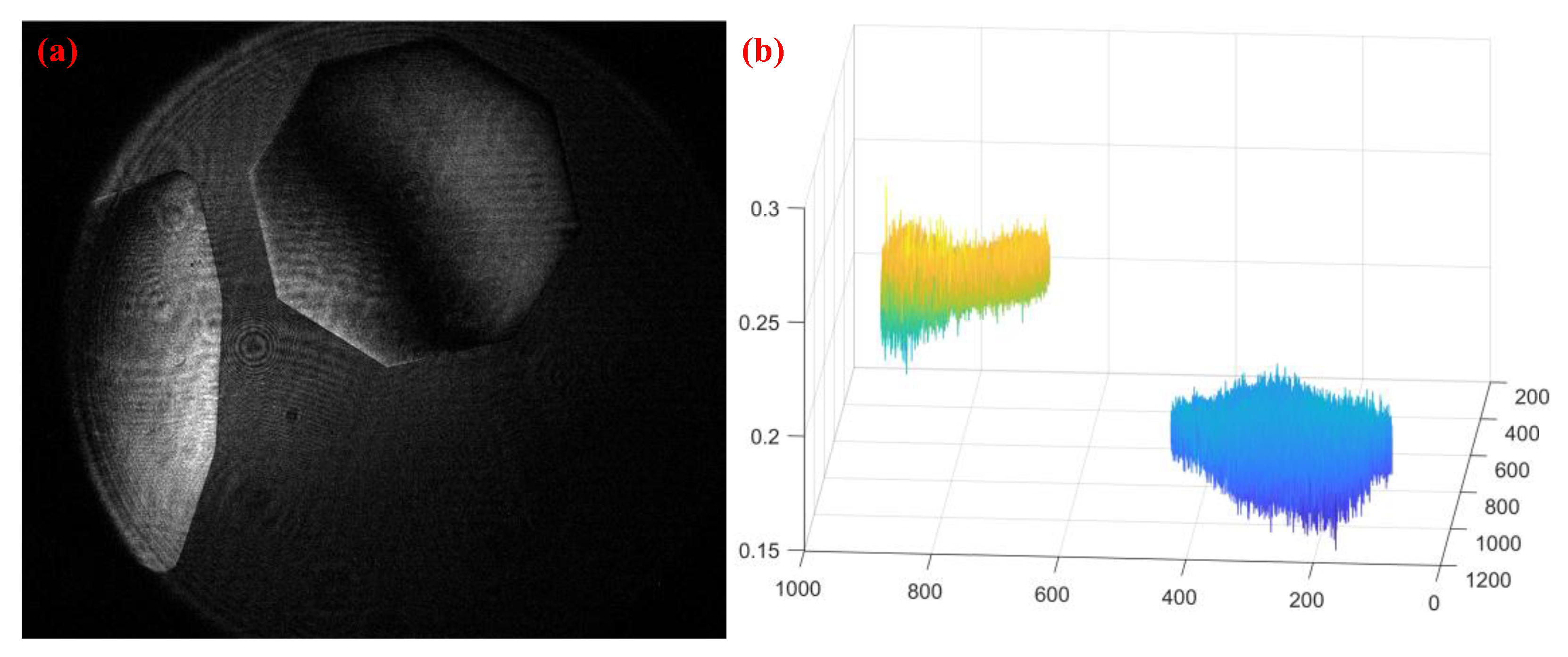
Adjust the segmented mirrors to being nearly co-phased, as shown in
Figure 6a; then, it needs to measure the residual piston as the piston value of the original case.
For measuring the piston, first, measure the wavefront data of different wavelengths using the phase-shifting interference method, as shown in
Figure 6b.
Then, calculate the OPD between two segments using Equation (4) for each wavelength.
Use the least squares method to calculate the slope and then calculate the piston using Equation (3)
Introduce an additional piston error using the 6-DOF parallel platform, and then repeat Steps 3 to 5; measure the piston again.
4.3. Small Piston Detection
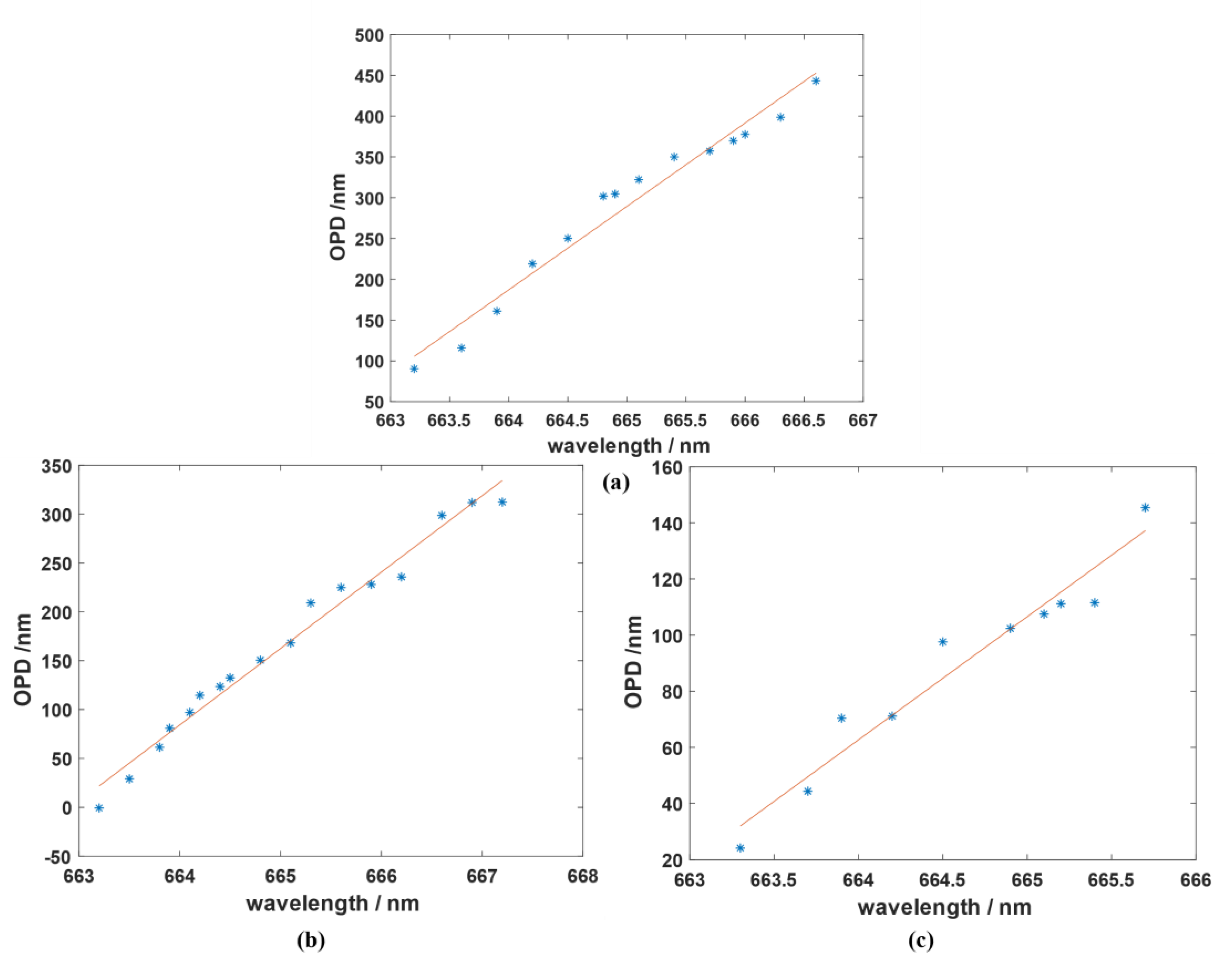
The 6-DOF parallel platform was used to input the piston error and adjust the segments; the measured wavelength was between 663 nm and 667.2 nm, and the wavelength sample interval was 0.3 nm. For each wavelength measurement, the interference fringe would be sampled 20 times and averaged to calculate the wavefront data; then, the wavefront data would be measured five times, and the final used data are the average values of the wavefront data. The segments should be first adjusted to nearly the co-phase, and then the existing piston error should be measured as the original value; this stage is called the original case in this study. For the small piston test, the piston error inputs were 10 μm and 20 μm compared with the original case, respectively. The result is shown in
Figure 7.
Figure 7a shows the original case in which the piston error calculated was about 14.620 μm.
Figure 7b shows the original case with a 10 μm piston input in which the piston error calculated was about 26.073 μm.
Figure 7c shows the original case with a 20 μm piston input in which the piston error calculated was about 34.121 μm. When one combines the original case and the other case, the deviation in the other case and the original case is about 11.453 μm and 19.501 μm, respectively; compared with the input value, the residual is 1.453 μm and −0.499 μm, respectively. The result indicates that under the conditions of our experiment, the small piston error (about dozens of micrometers) could be measured with a precision of about 1~2 μm, which is in accordance with the simulation results.
4.4. Large Piston Detection
As mentioned in
Section 3.2, the measurement range in the MWLF method depends on two factors: one is the size of the wavefront measurement error since this will damage the linearity of each linear area, and the boundary between each linear area will not be able to be distinguished; then, the data between the different linear areas will not be correctly corrected, causing the final measurement result to deviate from the true value. Another factor is the sample interval of the wavelength. Commonly, the larger the piston error, the larger the corresponding slope and the narrower the linear area. When the sample interval of the wavelength cannot ensure that there is enough valid data in each linear area, the information of the data point and the existing piston error will lose the corresponding relationship, resulting in piston errors that cannot be calculated. For each experimental system, based on the changes in these two factors, the maximum measurable range will also change, and the influencing factors affecting the wavefront measurement errors are relatively complex, changing with time, place, and the measurement environment. Therefore, the measurable range of the MWLF method, generally, can only be roughly determined through testing and is difficult to calculate theoretically.
For the large piston test in this study, in order to expand the measurable range, the wavelength sample interval was set to 0.1 nm, and the input piston errors were 100 μm and 300 μm, respectively. The results of the experiment can be seen in
Figure 7.
Figure 8a shows the original case, with the piston error calculated to be about −6.156 μm.
Figure 8b shows the original case with a −100 μm piston input, and the piston error was calculated to be about −105.727 μm.
Figure 8c shows the original case with a −300 μm piston input, and the piston error was calculated to be about −302.954 μm. Combining the original case and the other case, the deviation in the other case and the original case was about –100.429 μm and −296.438 μm, respectively, and compared with the input value, the residual was −0.429 μm and 3.562 μm, respectively.
5. Discussion
The measurement results in
Section 4.2 and
Section 4.3 show that, in a large measurable range, the accuracy of the MWLF method will not change significantly, which is different from the interferometry method based on the principles of synthetic wavelengths. The following is a brief analysis of the factors affecting the measurement accuracy of the MWLF method. The factors that affect the measurement accuracy can be roughly divided into two parts: wavefront detection accuracy and the sample interval of the measured wavelength.
The first is wavefront detection accuracy. Low wavefront detection accuracy will cause the wavefront test results of each segment to fluctuate, making the optical path differences between the segments fluctuate with each measurement. The reasons for the fluctuation in the optical path difference include the fluctuation in the actual optical path difference in the measurement (distance change caused by vibration, etc., refractive index change caused by airflow disturbances, and temperature and humidity changes), and the error in the interferometric measurement of the wavefront (wavefront detection error caused by interference fringe contrast, CCD noise, etc., and the solution error in the algorithm of unwrapping, Zernike coefficient fitting, etc.). Among them, the fluctuation in the actual optical path difference is generally a time-dependent error item. If all of the measured wavelengths or several measured wavelengths can be sampled at the same time, the influence can be greatly reduced, thus optimizing piston measurement accuracy, leading to a piston measurement precision greater than 300 nm.
Second is the effect of the wavelength sample interval. The difference in the wavelength sample interval essentially affects the number of effective data in each individual linear area. Usually, the minimum sample interval of the wavelength is selected with the goal of containing at least three effective data points in each linear area. However, the larger the amount of data involved in the calculation, the more stable the test results and the higher the test accuracy; however, sampling too much data will also increase the time cost of both the measurement and calculation, having high requirements in terms of the laser light source.
For the results shown in
Figure 8, it can be seen that, for a 300 μm piston input, compared with the other small input piston, the calculated error is relatively increased. In fact, when the existing piston error is close to the measurable range limit of the system, the piston measurement error will have an expanding trend. This is due to the fact that when the piston size is closer to the range limit, the effective data in each linear region will tend to be less, and then the influence of the wavefront measurement error on the linearity will be more obvious; thus the precision of the piston measurement will decrease. According to the simulation analysis and experimental experience, when the existing piston error is within 80% of the maximum measurable range, the detection error will not change significantly.
Generally, for the coarse phase process, the goal is to make the residual piston error less than 300 nm () so that it can enter the range of a single-wavelength detection and achieve detection accuracy at the nanometer level in the fine phase process, leading to all of the segment’s piston errors to be within to complete the co-phasing. Although, in the simulation and experiment sections of this study, the piston detection error is larger than 1 μm, considering that when the wavelength sample interval is more precise and a measurement environment with a smaller wavefront detection error is provided, this accuracy can be optimized to a satisfactory value; thus, the MWLF method can independently complete the coarse co-phase process of the segmented mirrors compared with the synthetic wavelength method, since MWLF will not expand the piston measurement error with an increased range. Therefore, it can be considered to be a more suitable coarse co-phase detection method.
6. Conclusions
In this study, a coarse co-phasing method based on the relationship between the optical path difference in different wavelengths between the segments has been proposed, which is called the multiwavelength wavefront linear fit method.
The simulation results indicate that the MWLF method can maintain relatively high detection accuracy in a large dynamic range under the conditions of a large measurement error when the wavefront detection error has a random distribution of and the wavelength sample interval is 0.1 nm, the measurement range can reach about 500 μm, and the measuring accuracy can reach approximately 1 μm RMS. When the wavefront detection error is under the conditions of , the wavelength sample interval is 0.1 nm or , the wavelength sample interval is 0.01 nm, and the measurement accuracy of the piston errors can be better than 300 nm RMS, which satisfies the needs of the coarse phasing progress; thus, the segments can successfully converge to the fine phasing process via the MWLF method.
In the experimental results, for the 10 μm,20 μm, and 100 μm input piston errors, the piston measurement accuracy of the MWLF method is about 1.5 μm, when the measured piston is far from the measurable range, and for the input of 300 μm, the precision is about 4 μm, since this piston is near the range limit. According to the simulation results, it is reasonable to assume that if the laser source has a higher wavelength resolution or the influence of the wavefront measurement error is reduced, the detection accuracy for piston errors using the MWLF method can be optimized to within 300 nm, which can meet the requirements of the transition from coarse phasing to fine phasing. Meanwhile, the MWLF method has advantages in terms of detection range and speed and can accelerate the convergence rate of the coarse phasing process. Therefore, it can be considered that this method has significant application potential in the field of co-phasing segmented mirrors.
Author Contributions
Conceptualization, R.Q.; methodology, R.Q.; formal analysis, R.Q. and Z.Y.; investigation, R.Q. and Z.Y.; resources, Y.L.; data curation, R.Q. and Z.Y.; writing—original draft preparation, R.Q.; writing—review and editing, R.Q.; visualization, R.Q.; supervision, Y.L.; project administration, Y.L.; funding acquisition, Y.L. All authors have read and agreed to the published version of the manuscript.
Funding
This research was funded by the Major Program of the National Natural Science Foundation of China (grant no. 42192582), and the National Key R&D Program of China (grant no. 2022YFB3902000 and 2016YFB0500400).
Data Availability Statement
Data underlying the results presented in this paper are not publicly available at this time but may be obtained from the authors upon reasonable request.
Conflicts of Interest
The authors declare no conflict of interest.
References
- Wang, Q. Research framework of remote sensing monitoring and real-time diagnosis of earth surface anomalies. Acta Geod. Cartogr. Sin. 2022, 51, 1141–1152. [Google Scholar] [CrossRef]
- Yaitskova, N.; Dohlen, K.; Dierickx, P. Analytical study of diffraction effects in extremely large segmented telescopes. J. Opt. Soc. Am. A 2003, 20, 1563–1575. [Google Scholar] [CrossRef] [PubMed]
- Yaitskova, N.; Dohlen, K. Tip-tilt error for extremely large segmented telescopes: Detailed theoretical point-spread-function analysis and numerical simulation results. J. Opt. Soc. Am. A 2002, 19, 1274–1285. [Google Scholar] [CrossRef] [PubMed]
- Quirós-Pacheco, F.; Schwartz, D.; Das, K.; Conan, R.; Bouchez, A.H.; Irarrazaval, B.; McLeod, B.A. The Giant Magellan Telescope phasing strategy and performance. In Proceedings Volume 10700, Ground-Based and Airborne Telescopes VII, Proceedings of the SPIE Astronomical Telescopes + Instrumentation, Austin, TX, USA, 10–15 June 2018; SPIE: Bellingham, WA, USA, 2018. [Google Scholar] [CrossRef]
- Sanders, G.H. The Thirty Meter Telescope (TMT): An International Observatory. J. Astrophys. Astron 2013, 34, 81–86. [Google Scholar] [CrossRef] [Green Version]
- Diolaiti, E.M.; Ciliegi, P.; Abicca, R.; Agapito, G.U.; Arcidiacono, C.A.; Baruffolo, A.; Bellazzini, M.; Biliotti, V.; Bonaglia, M.A.; Bregoli, G.; et al. MAORY: Adaptive optics module for the E-ELT. In Proceedings Volume 9909, Adaptive Optics Systems V, Proceedings of the SPIE Astronomical Telescopes + Instrumentation, Edinburgh, UK, 26 June–1 July 2016; SPIE: Bellingham, WA, USA, 2016. [Google Scholar] [CrossRef]
- Li, Y.; Wang, S. Diagnosing piston error from hyperspectral image with extended scene. Opt. Lasers Eng. 2023, 161, 107375. [Google Scholar] [CrossRef]
- Li, X. The piston error recognition technique used in the modified Shack–Hartmann sensor. Opt. Commun. 2021, 501, 127388. [Google Scholar] [CrossRef]
- Sato, S.; Mizutani, T. Cross-fringe piston sensor for segmented optics. Appl. Opt. 2022, 61, 3972–3979. [Google Scholar] [CrossRef]
- Yang, L.; Yang, D.; Yang, Z.; Liu, Z. Co-phase state detection for segmented mirrors by dual-wavelength optical vortex phase-shifting interferometry. Opt. Express 2022, 30, 14088–14102. [Google Scholar] [CrossRef]
- Zhao, W. Piston detection in segmented telescopes via multiple neural networks coordination of feature-enhanced images. Opt. Commun. 2022, 507, 127617. [Google Scholar] [CrossRef]
- Shi, F.; King, B.M.; Sigrist, N.; Basinger, S.A. NIRCam Long Wavelength Channel grisms as the Dispersed Fringe Sensor for JWST segment mirror coarse phasing. In Proceedings Volume 7010, Space Telescopes and Instrumentation 2008: Optical, Infrared, and Millimeter, Proceedings of the SPIE Astronomical Telescopes + Instrumentation, Marseille, France, 23–28 June 2008; SPIE: Bellingham, WA, USA, 2008. [Google Scholar]
- Qin, R.; Yin, Z.; Ke, Y.; Liu, Y. Large Piston Error Detection Method Based on the Multiwavelength Phase Shift Interference and Dynamic Adjustment Strategy. Photonics 2022, 9, 694. [Google Scholar] [CrossRef]
| Disclaimer/Publisher’s Note: The statements, opinions and data contained in all publications are solely those of the individual author(s) and contributor(s) and not of MDPI and/or the editor(s). MDPI and/or the editor(s) disclaim responsibility for any injury to people or property resulting from any ideas, methods, instructions or products referred to in the content. |
© 2023 by the authors. Licensee MDPI, Basel, Switzerland. This article is an open access article distributed under the terms and conditions of the Creative Commons Attribution (CC BY) license (https://creativecommons.org/licenses/by/4.0/).


