Article

Modulation Format Identification and OSNR Monitoring Based on Multi-Feature Fusion Network

1
School of Electronics and Information Engineering, Hebei University of Technology, Tianjin 300401, China
2
Tianjin Key Laboratory of Electronic Materials & Devices, Tianjin 300401, China
3
Hebei Provincial Key Laboratory of Advanced Laser Technology and Equipment, Tianjin 300401, China
*
Author to whom correspondence should be addressed.
Photonics 2023, 10(4), 373; https://doi.org/10.3390/photonics10040373
Submission received: 19 February 2023 / Revised: 16 March 2023 / Accepted: 24 March 2023 / Published: 27 March 2023
(This article belongs to the Topic Fiber Optic Communication)

Abstract

:
In this paper, we propose a multi-feature fusion network (MFF-Net) for a modulation format identification (MFI) and optical signal-to-noise ratio (OSNR) monitoring scheme. The constellation map data used in this work comes from five modulation formats, namely 56 Gbit/s 4/8 phase shift keying (PSK) and 16/32/64 quadrature amplitude modulation (QAM). The constellation maps are input to one branch network of the MFF-Net, and then the constellation maps are processed by horizontal projection and used as input to another branch network as a way to fuse the two image features. The results show that the scheme achieves 100% MFI accuracy and 98.82% OSNR monitoring accuracy for the five modulation formats. In addition, the performance of MFF-Net and binarized convolutional neural network (B-CNN), visual geometry group network (VGG-Net), and traditional weighted multi-task learning (EW-MTL) are compared to present the superiority of the method. The effect of model structure on MFF-Net is also discussed. The robustness of the model is also evaluated for different transmission distances and bit rates.

1. Introduction

With the continuous progress and evolution of emerging technologies, including artificial intelligence and the mobile Internet, modern society has been pushed into the era of the “Internet of Everything”. Coherent optical communication technology has also become increasingly sophisticated. Flexible and effective optical performance monitoring (OPM) [1,2,3,4] techniques are playing an increasingly prominent role in ensuring the correct and efficient transmission of signals. Optical signal-to-noise ratio (OSNR) monitoring is particularly critical for the OPM of coherent links since the OSNR is used to measure how much the signal is disturbed by noise. Furthermore, OSNR monitoring requires information about the input signal type. Therefore, modulation format identification (MFI) is essential.
An effective means to realize MFI and OSNR monitoring is deep learning (DL) [5,6], which has been widely used in optical communication [7,8,9,10,11,12]. Reference [13] proposed a likelihood-based approach for orthogonal frequency division multiplexing with index modulation systems to achieve blind MFI. However, it requires much prior knowledge and is relatively complex to compute. An MFI method based on signal amplitude was proposed in [14], which can achieve favorable performance utilizing only a small number of samples, yet it is not applicable to M-PSK classification. Liu et al. used a nonlinear power conversion scheme [15] that provides high identification accuracy. However, it requires a longer fast Fourier transform for higher-order modulation formats. In Ref. [16], the authors implemented MFI with frequency domain features, i.e., magnitude variance and fast Fourier transform, subject to a strict set of the threshold. In Ref. [17], Khan et al. made asynchronous amplitude histograms using amplitude features extracted by asynchronous sampling and then trained artificial neural networks with a large amount of data. Although the method provides high accuracy, artificial neural networks do not apply to complex situations. In addition, the use of amplitude characteristics has its limitations and is only valid for QAM modulation formats. The constellation maps of the received signals in [7] were taken as input to the convolutional neural network (CNN), which realized an MFI higher than 95% as well as an OSNR estimation with small errors. However, the computational complexity of this algorithm is high. The CNN was trained using the eye diagram in [18] to obtain MFI without human intervention, yet its need for timing recovery led to high costs. In Ref. [10], the authors used CNN and asynchronous delay-tap plots for 16QAM, 32QAM, and 64QAM to perform a study on the subject and verified its efficiency experimentally. However, it does not have the advantage of low cost because two samples are taken. Wang et al. presented the adoption of the frequency domain information of the signal at the receiver as the input features of the long short-term memory (LSTM) neural network to accomplish OSNR monitoring [19]. Ref. [20] trained data using LSTM neural networks to perform OSNR monitoring without prior knowledge. However, the long- and LSTM neural network does not fully utilize the frequency domain features and has a high memory requirement, which leads to a high research cost. In Ref. [21], Xia et al. employed a transfer learning-based assisted deep neural network to train the amplitude histogram and experimentally verified the effectiveness of this scheme for OSNR monitoring. However, this was not applicable to the phase modulation format. In Ref. [22], a CNN was applied to analyze the constellation maps of six modulation formats from an image processing perspective, and 100% MFI accuracy was obtained. R. A. Eltaieb et al. in [23] proposed two MFI methods that perform singular value decomposition and Radon transforms on constellation graphs and validated them using three traditional classifiers, namely support-vector machine, K-nearest neighbor, and decision tree. Zhang et al. proposed a lightweight two-stage deep neural network for the MFI scheme [24]. Shen et al. used CNNs to perform OSNR estimation and achieved end-to-end monitoring [25]. Reference [26] put forward a graph-based modulation format identification method to accurately classify different input signal types using trajectory information. However, the main limitation of the DL-based approaches described above is that they focus only on exploiting the network rather than integrating information between diverse features. To address this issue, DL-based multi-feature fusion [27] is an effective technique, and in reference [28], Zhang et al. fused features learned from their network structure and attribute information for node classification in a communication system.
This paper proposes a scheme based on a multi-feature fusion network (MFF-Net) that combines the constellation and horizontal projection features to achieve MFI and OSNR monitoring. Firstly, the system is simulated for five modulation formats, which are 4/8 phase-shift keying (PSK) and 16/32/64 quadrature amplitude modulation (QAM), respectively. Constellations are collected for five modulation formats under different OSNRs. The collected constellation maps are fed into a branch network of MFF-Net. Then, they are processed using the horizontal projection method, and the projected images are used as input to another branch network. Subsequently, two branching networks are utilized to extract 22 high-level features from the two types of images, respectively. The features learned from the two types of images are integrated using multi-feature fusion techniques to obtain the complementary advantages between the dissimilar features. In this study, the MFI and OSNR monitoring performance of the MFF-Net model is validated and analyzed. We compare the performance of MFF-Net, B-CNN [29], VGG-Net [30], and EW-MTL [2] using 2 aspects: the number of parameters and OSNR precision. The findings of the simulation demonstrate that the method enables MFI and OSNR monitoring of the received signal with high accuracy. The effect of the image resolution network structure on the identification accuracy is also analyzed. Furthermore, we assess the robustness of MFF-Net and conclude it is robust to transmission distances and high bit rates.
The structure of the remaining sections of this paper is as follows: Section 2 specifies the scheme to implement MFI and OSNR monitoring. Section 3 describes the simulation system setup and the origin of the data set. The simulation results are discussed and analyzed in Section 4. Finally, Section 5 draws conclusions.

2. Proposed Scheme

In this section, the data pre-processing operation is performed for the constellations collected by the simulation system, and the procedure for the model is elaborated.

2.1. Data Pre-Processing

The binary image processing of the constellation diagram should be performed before the horizontal projection. The formula for binarization is shown in Equation (1):
T = { 255 ,   A r B 0 ,   e l s e
where r is the pixel point on the constellation diagram, and A and B refer to the set color threshold. Image binarization means that the entire image is rendered with a distinct black-and-white effect. After the binarization of constellations, the amount of data can be reduced, and post-processing can be simplified.
The principle of horizontal projection is to circulate each row of the image, determine whether the pixel value of each column is black or not in turn, and calculate the number of all black pixels in that row. The size of the image is H × W, where H is the height and W is the width. The calculation procedure of horizontal projection is in Equation (2):
S ( i ) = j = 1 H I ( i , j )
where (i, j) is the position of the pixel point, i∈(1, H), j∈(1, W), and I (i, j) represents the pixel value.
Figure 1 demonstrates the constellation diagrams captured for the five modulation formats at an OSNR of 25 dB, along with the corresponding horizontal projection diagrams. After horizontal projection, QPSK, 8PSK, 16QAM, 32QAM, and 64QAM change from 4, 8, 16, 32, and 64 constellation point features to 2, 3, 4, 6, and 8 peaks, respectively, which makes the features more obvious, thus making it easy for the model to extract features and improve the accuracy.

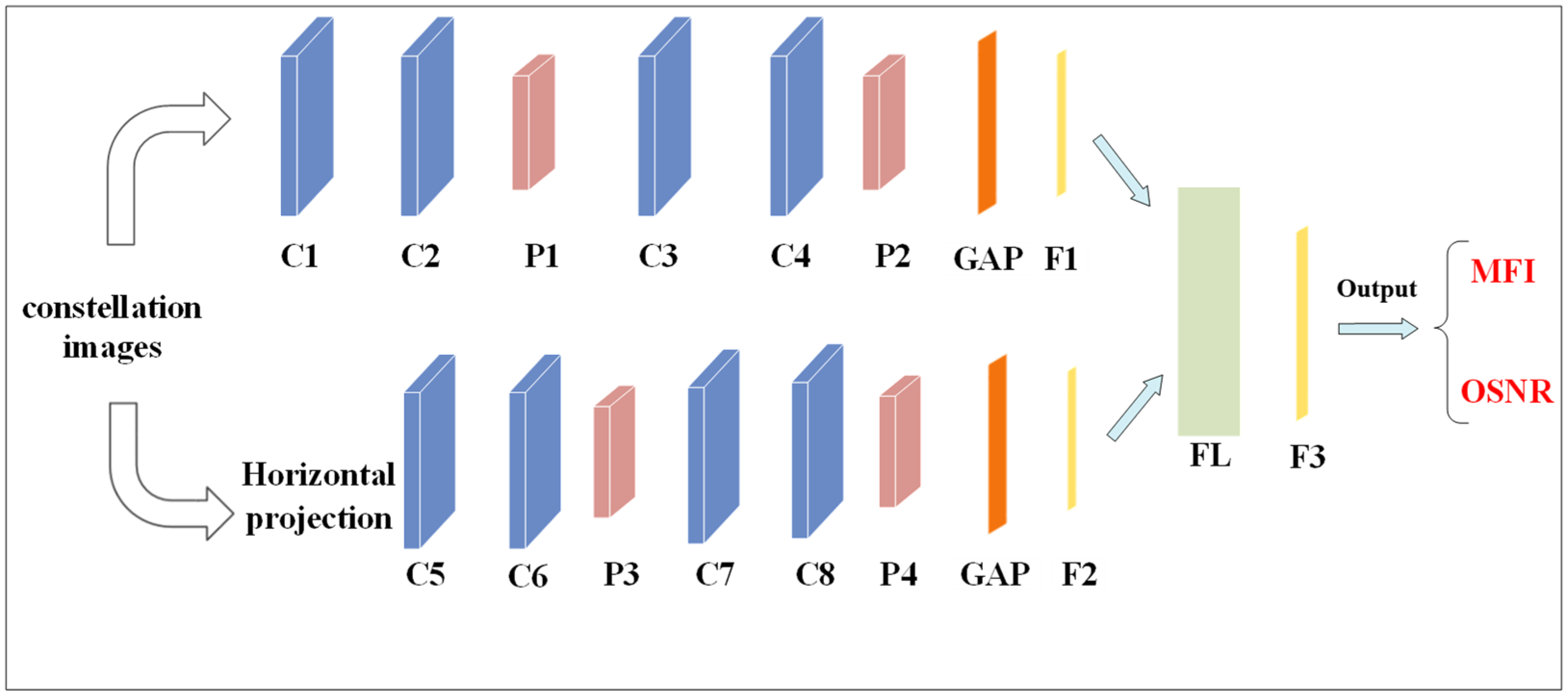
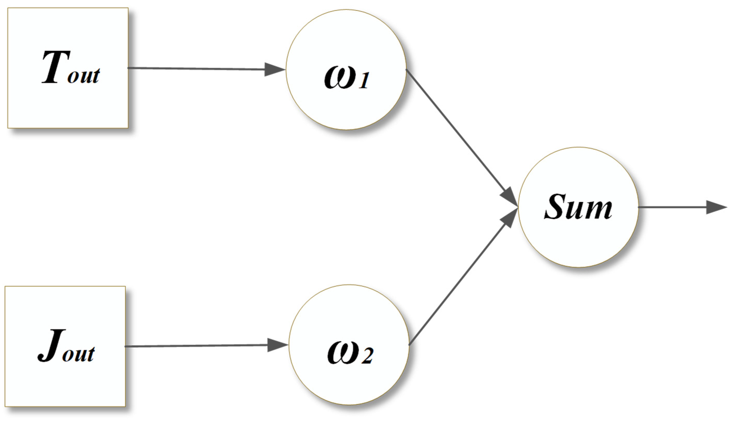
2.2. System Structure
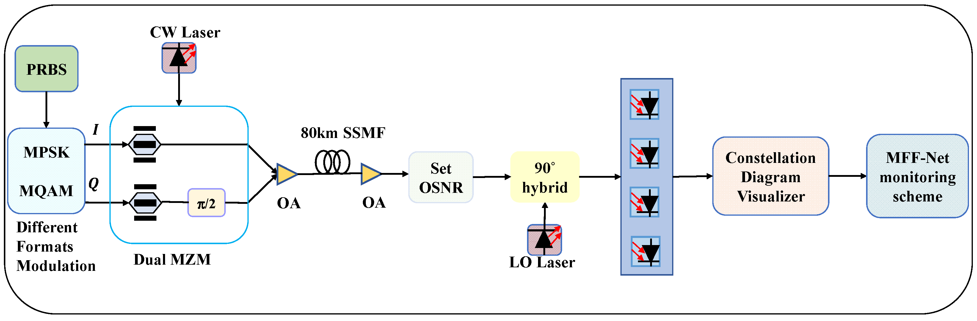
Multi-feature fusion plays a significant function in the computer vision field. Figure 2 describes the schematic architecture of the MFF-Net model used in this work, which consists of two branch networks. The constellation map is input to one of the branch networks of the MFF-Net, and the image is then used as input to another branch network after horizontal projection processing. The constellation maps are used as the input to retain more information about the modulation format, while the utilization of horizontal projection maps can enhance the constellation map features to improve the classification accuracy. Both branch networks comprise 4 convolutional layers, 2 pooling layers, 1 global average pooling (GAP) layer, and 1 fully connected layer. The GAP layer replaces the flattening layer to simplify the network’s complexity and prevent overfitting. The feature fusion layer (FL) fuses the feature information extracted from the two branch networks and outputs the classification results through the SoftMax classifier. The number of filters in convolutional layers C1, C2, C3, and C4 is 16, 32, 64, and 128, respectively, and the size of the convolutional kernel is 3 × 3. The pooling layers P1 and P2 have a kernel size of 2 × 2 with a stride of two. The neuron counts in fully connected layers F1 and F2 are 256 and 256, respectively. The parameters of each layer in another branch network are the same as above. F3 is the classification layer. In addition, the use of dropout and the activation function ReLU (instead of sigmoid) serves to prevent overfitting.
For each modulation format, we consider 11 (15–25) OSNR values. Additionally, the constellation and horizontal projection samples with 480 × 480 pixels are considered inputs to the MFF-Net model. Initially, the input image size is adjusted to 100 × 100, and then the constellation diagrams are binarized to grayscale to improve the calculation speed of the system. Before the training of the model, the input image is first normalized to reduce the influence of the geometric transformation of the image. The normalization process is given in Equation (3):
X * = ( X - m i n ) / ( m a x - m i n )
where X* refers to the normalized image data, X means the image pixel point value, and min and max refer to the maximum and minimum values of the image pixels, respectively.
The MFF-Net model proposed in this work contains two identical branching convolutional neural networks that extract the features of the constellation and horizontal projection accordingly. Equation (4) presents the formula of the convolutional layer:
K Conv = K F + 2 P S + 1
where K × K is the input image size for the convolutional layer, and KConv × KConv is the output image size of the convolutional layer. F × F is the convolutional kernel size. S is the stride, and P is the padding size. The activation function is the nonlinear rectification unit ReLU.
After the features are extracted by convolutional layers, the feature maps are passed to the max pooling layer, which minimizes model parameters, reduces the number of dimensions, improves the efficiency of the network, and prevents overfitting while retaining the features extracted by the convolutional layers as much as possible. The formula for max pooling is provided in the following Equation (5):
K P o o l i n g = K F S + 1
where K × K is the input image size for the pooling layer and Kpooling is the output image size of the pooling layer.
When the two features go through convolution and pooling operations, respectively, they feed into the fully connected layer through the feature fusion layer. In the MFF-Net model, the constellation map feature Tout extracted by a branching network contains more information about the location of constellation points, while the horizontal projection feature Jout extracted by another branching network has more semantic information. Figure 3 presents the feature fusion module that reasonably fuses the feature information of the two branch networks and introduces adaptive feature weights. The model automatically decides its weight parameters based on the feature distribution of the data and fuses the features at the fusion layer. The fused features Cf are calculated using Equation (6).
C f = ω 1 × T o u t ω 2 × J o u t
where ⊕ represents the sum fusion method; the weights ω1 and ω2 are obtained from Equation (7).
ω i = e α i j e α j ( i = 1 , 2 ; j = 1 , 2 )
where ωi is the normalized weight and ∑ ωi = 1, αi is the initialized weight parameter. αi is added to the parameters updated by the optimizer so that αi is optimized in the direction of minimizing the loss function.
Lastly, the SoftMax classifier is utilized to output the modulation format and OSNR information. This paper integrates the features by adopting a multi-feature fusion technique, which can fully utilize the advantages of dissimilar features to improve the accuracy of MFI and OSNR monitoring.

3. Simulation Setup

We used the OptiSystem V15.0 simulator to build a coherent optical communication system with 56 Gbit/s QPSK/8PSK/16QAM/32QAM/64QAM five modulation formats. Figure 4 shows the simulation setup of the coherent optical communication system. For each modulation format, the OSNR was selected in the range of 15 to 25 dB. We adequately captured the possible cases of the same category for the sake of guaranteeing the abundance and diversity of the dataset. The simulation system repeatedly collected 200 constellations for each category of OSNR values, with all parameters of the system being invariant. The pixel size was 480 × 480 for the constellations captured by the constellation diagram analyzer. At the transmitter terminal, a pseudo-random binary sequence (PRBS) of length 217 was mapped into MQAM and MPSK signals, and the electrical signals were generated by an arbitrary waveform generator. A continuous wave (CW) laser with a center frequency of 193.1 THz, a line width of 0.1 MHz, and a power of 10 dBm was utilized to generate the optical carrier signal. It was required by the system to drive the dual Mach-Zehnder Modulator (Dual MZM). The modulated signal was transmitted through a standard single-mode fiber (SSMF) with a length of 80 km, an attenuation of 0.2 dB/km, and a dispersion of 16.75 ps/nm/km. Optical amplifiers (OA) were deployed to make up for the losses generated during transmission. At the optical receiving end, the coherent receiver contained a photodetector. The local oscillator (LO) operated at 1550 nm with a linewidth of 0.1 MHz. It mixed with the optical signal and subsequently converted the optical signal into an electrical signal using the photodetector. The constellation diagrams of the electrical signals were analyzed and collected using a constellation diagram analyzer. The generated constellation images were then sent to the MFF-Net-based digital signal processing module.
Based on this system, the gathered constellation diagrams are pre-processed and then monitored for MFI and OSNR using the proposed scheme.

4. Results and Discussion

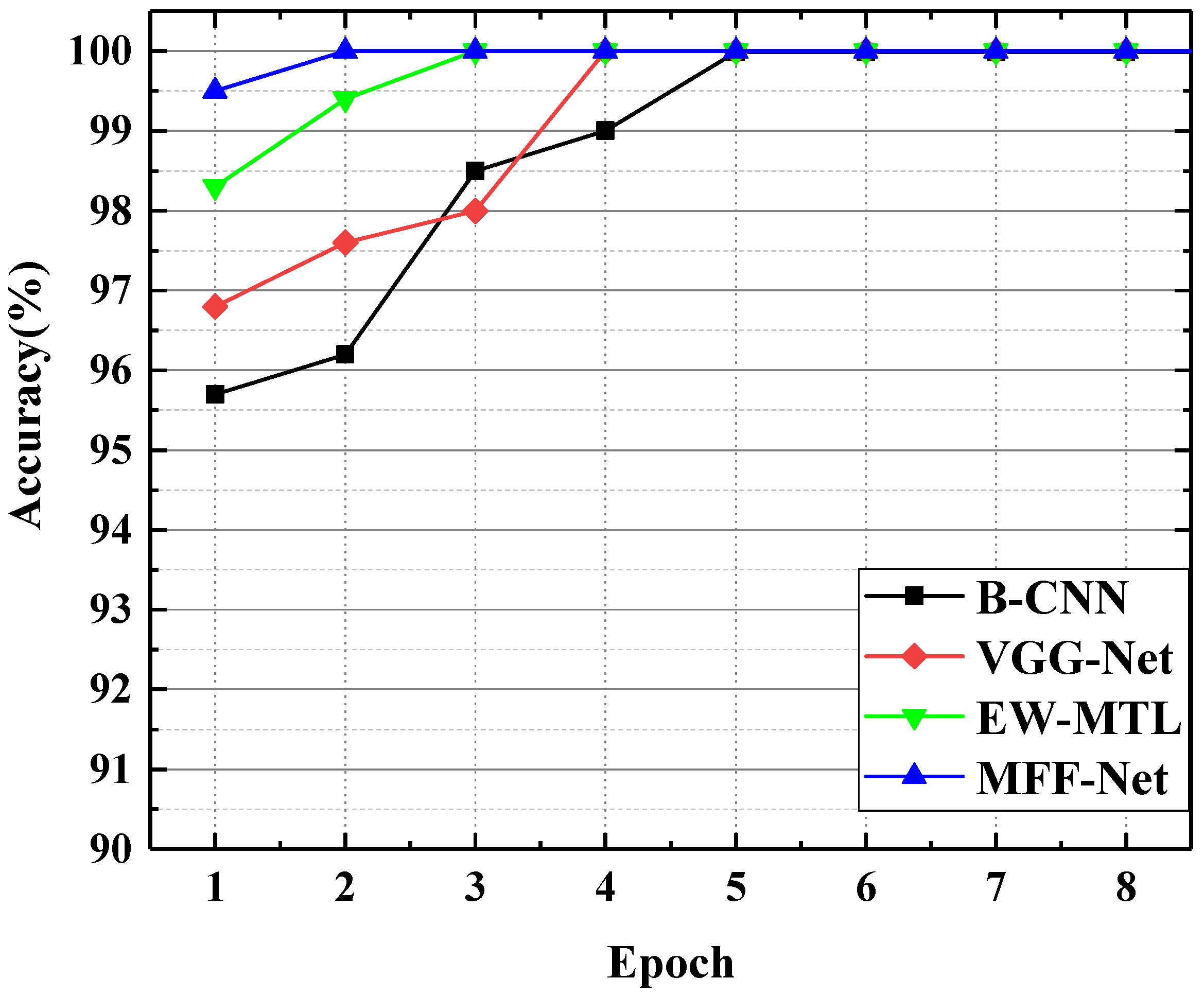
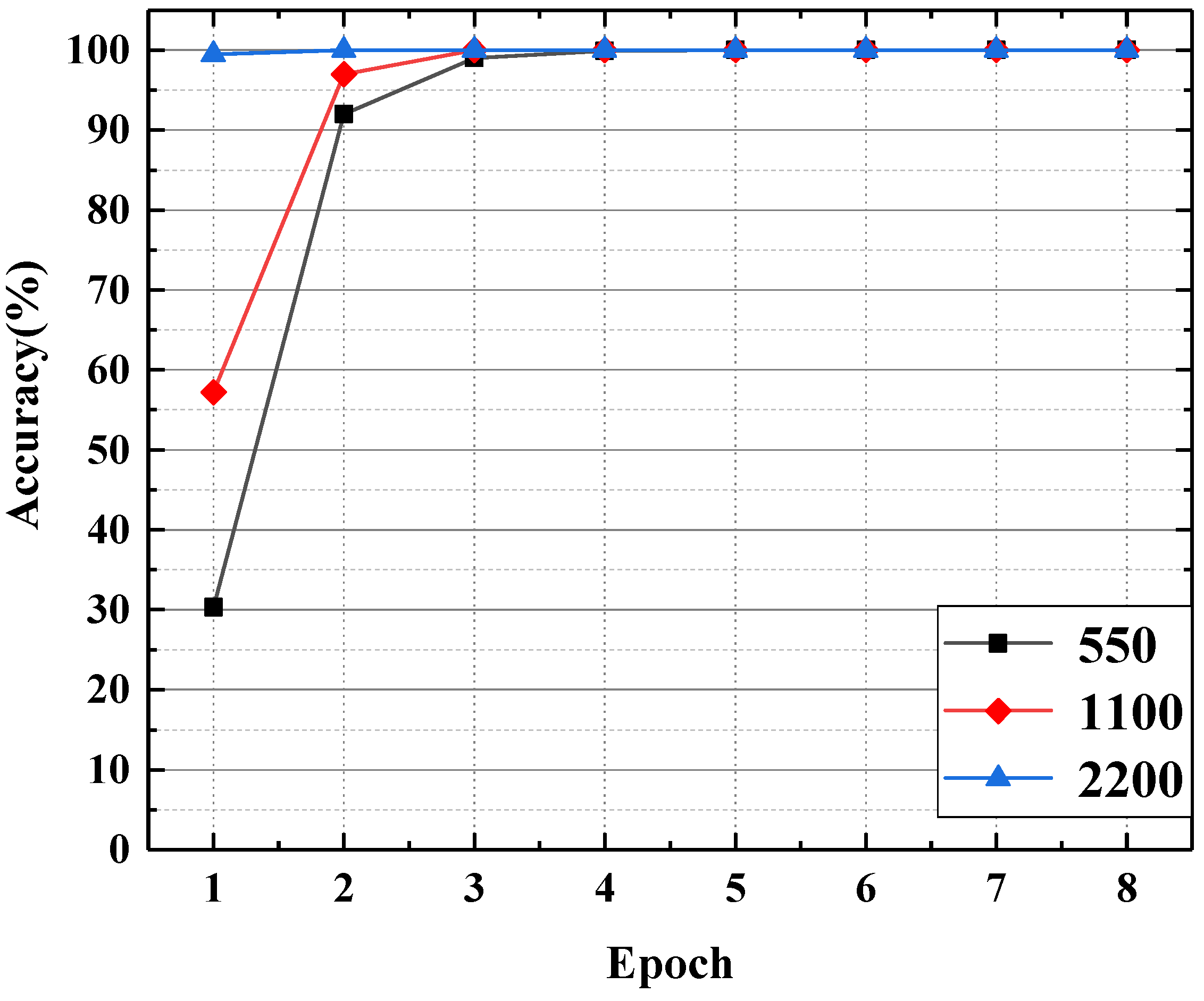
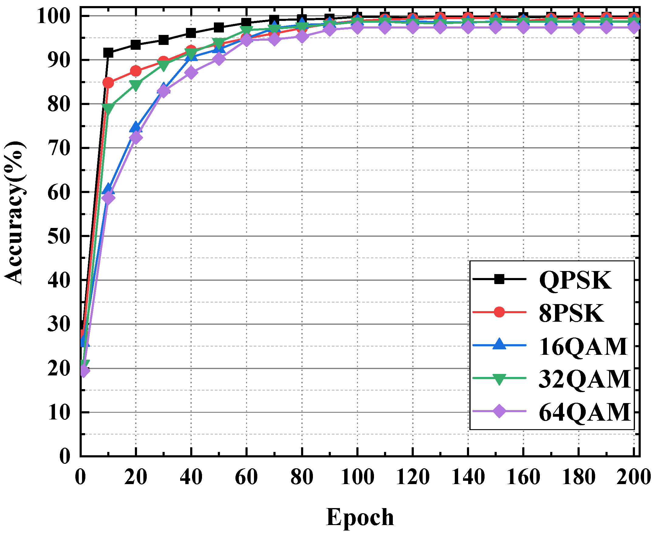
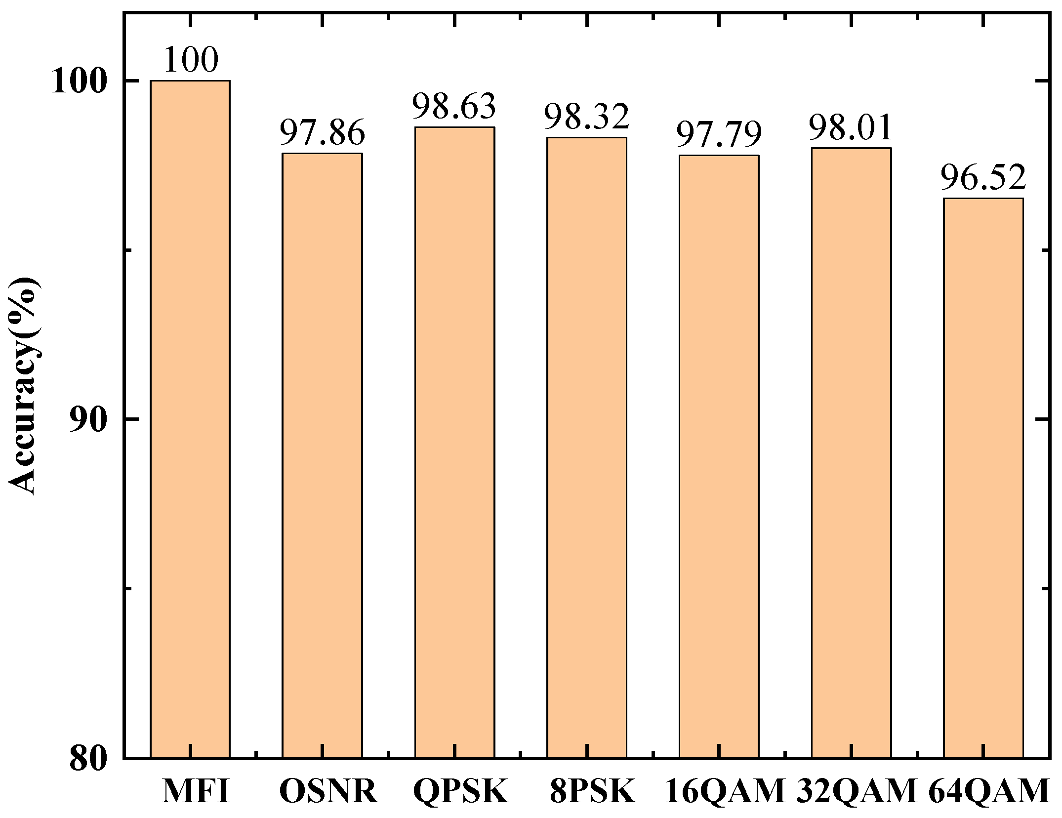
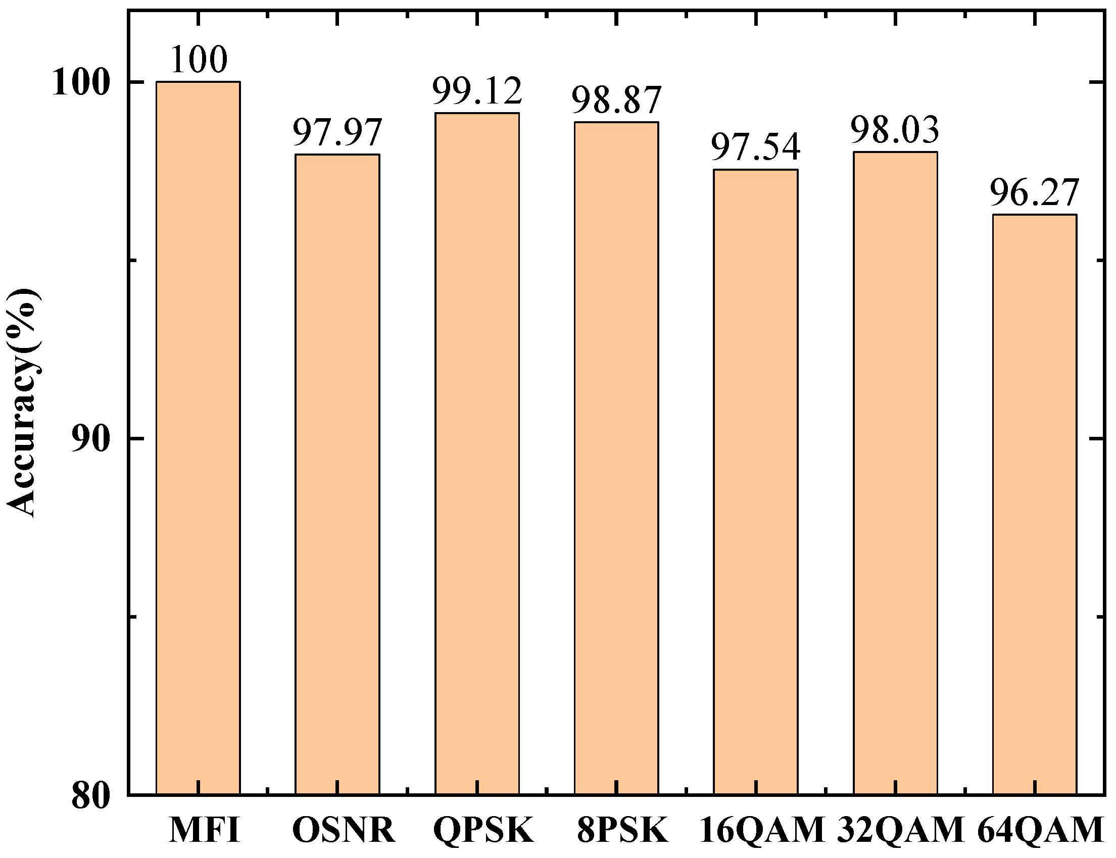
4.1. Modulation Format Identification

Considering the effectiveness of the proposed scheme, the performance of MFF-Net on MFI is first investigated.
In Figure 5, the results of MFI are shown, comparing the proposed scheme in this study to a B-CNN, VGG-Net, and EW-MTL. The OSNR range for QPSK/8PSK/16QAM/32QAM/64QAM in this part is 15–25 dB. The dataset used consists of 200 × 11 × 5 = 11,000 constellation diagrams and training and test sets in the proportion of 70% and 30%, where 200 refers to 200 constellation maps collected at each OSNR, while 11 and 5 refer to the 11 OSNRs and 5 modulation formats we set up, respectively. Additionally, the five types of modulation format constellations are mixed and casually disrupted to be used for training and testing. All four models perform accurate MFI, with MFF-Net, VGG-Net, and EW-MTL all achieving 100% accuracy and B-CNN reaching 99.9%. When the epoch is 1, the MFI results for MFF-Net, EW-MTL, VGG-Net, and B-CNN are 99.5%, 97.6%, 96.8% and 95.7%, respectively. In addition, the accuracy of several models increases with increasing epoch, such that MFF-Net first reaches 100% at the second epoch, and EW-MTL, VGG-Net and B-CNN achieve their highest accuracies at 3, 4, and 5 epochs, respectively. According to the simulation results, although all of the models can achieve a high-accuracy MFI, MFF-Net undergoes the least number of iterations and can achieve 100% accuracy the fastest. Therefore, this proves that our designed MFF-Net can achieve faster convergence and is effective. Compared to OSNR monitoring, MFI is easier to identify and achieve 100% accuracy with due to the distinctly disparate characteristics of constellations for different modulation formats.
We reduced the sample size of constellation maps for each format from 2200 to 1100 and 550, respectively, to observe the performance of MFF-Net in terms of MFI and to discuss the robustness [31] of the proposed system. The accuracy rates under different epochs are presented in Figure 6. The MFI accuracy is positively associated with the sample size and increases significantly with the growth of the number of samples. The accuracy at all sample sizes increases with increasing epochs and eventually reaches 100%. Therefore, we can obtain that the same results can be achieved for large sample sizes by increasing the epoch in the case of small samples. This proves the excellent validity of MFF-Net for MFI.

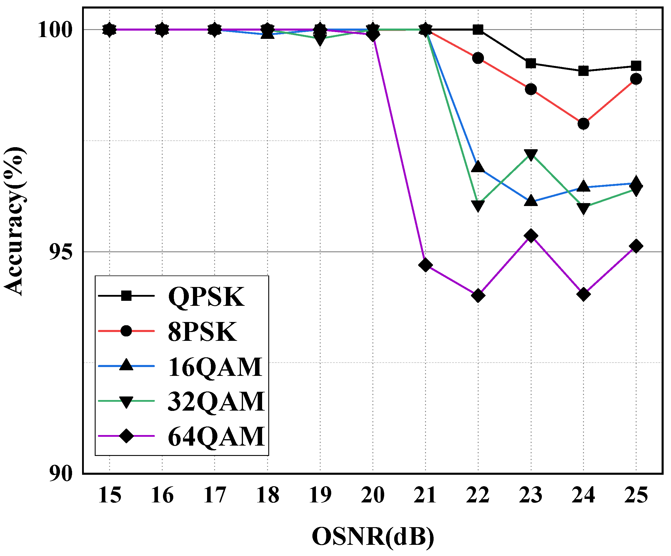
4.2. OSNR Monitoring

Simultaneously, this work examines the performance of OSNR monitoring based on the MFF-Net model. The accuracy of OSNR monitoring for different epochs is given in Figure 7. It is clear that the OSNR accuracy of the five formats increases with the epoch. When the epoch is less than 100, the monitoring accuracy increases rapidly with the increase in the epoch. In particular, QPSK is the first to achieve high monitoring accuracy. As the modulation format order increases, the accuracy changes more slowly with the epoch. In addition, all five modulation formats achieve an accuracy of more than 97% when the epoch reaches 100. Finally, when the epoch reached 200, the accuracy of QPSK, 8PSK, 16QAM, and 32QAM was 99.77%, 99.53%, 98.72%, and 98.68%, respectively. 64QAM carries more feature information, so its recognition accuracy changes the slowest with the epoch. However, the accuracy of 64QAM also reaches 97.38% at the 200th epoch. This proves the excellent effectiveness of MFF-Net in monitoring OSNR.
To demonstrate the advantage of MFF-Net, OSNR estimation is also performed for the other three models, B-CNN, VGG-Net, and EW-MTL, as illustrated in Figure 8. The histogram reveals that MFF-Net outperforms all the other algorithms. The OSNR accuracy of MFF-Net ranges from 97.38 to 99.77%. On average, the accuracy is 98.82%. The OSNR accuracy of EW-MTL has a range of 97.03~99.51% with a mean accuracy of 98.41%, and the OSNR accuracy of VGG-Net ranges from 96.85% to 99.01% with a median accuracy of 98.16%. The range of B-CNN is 95.33~98.68%, and the mean accuracy is 97.38%. Based on the results, it can be inferred that MFF-Net has the best performance, while EW-MTL has a slightly worse performance than MFF-Net, and VGG-Net is not as good as EW-MTL but better than B-CNN.
In addition, the complexity of the models is considered. Since there are too many variables describing the time complexity of deep learning instead of describing it accurately, we compared the accuracy and the number of parameters of these four models.
The number of covariates for each convolutional layer can be calculated using Equation (8):
P C o n v = n × ( k × k × c + 1 )
The number of parameters of the fully connected layer can be obtained by Equation (9):
P f c = n × ( c + 1 )
where PConv and Pfc represent the number of parameters of the convolutional layer and fully connected layer, respectively. The dimension of the convolution kernel is k × k, where c and n correspond to the number of channels in the input feature map and the output feature map for the layer, respectively.
As shown in Table 1, the OSNR monitoring accuracies of MFF-Net, B-CNN, VGG-Net, and EW-MTL on this dataset are 98.82%, 97.38%, 98.16%, and 98.41%, respectively, corresponding to the number of parameters 2.64 × 10⁵, 1.63 × 10⁸, 4.27 × 10⁶, and 4.76 × 10⁵. In addition, we also compared CNN and LSTM, which are shown in the last two columns of Table 1. The OSNR monitoring accuracy is 97.13% and 98.53%, respectively, and the number of parameters is 2.51 × 10⁶ and 4.80 × 10⁵, correspondingly. There is no significant advantage compared with the model in this paper, both in terms of the number of parameters and accuracy. In the MFF-Net model, we replaced the flattening layer with the global average pooling layer, which greatly reduces the number of model parameters. It can be concluded that MFF-Net has the lowest number of parameters and the highest accuracy rate, which is superior compared with other models.
Figure 9 signifies the OSNR monitoring results for the five modulation formats. It can be clearly seen that at low OSNRs (15–21 dB), QPSK, 8PSK, 16QAM, and 32QAM all achieve 100% accuracy. This is because changing the OSNR value in this context results in a very obvious change in the constellation maps. Moreover, the horizontal projection processing method is able to characterize this change clearly, which in turn results in high-accuracy OSNR monitoring by the MFF-Net model. When the OSNR increases to a certain level, the constellation diagram and horizontal projection diagram no longer change significantly with the change of OSNR, and the constellation diagram and horizontal projection characteristics of adjacent OSNRs are not distinctly different, thus making it more difficult for MFF-Net to perform OSNR monitoring and resulting in a decrease in the monitoring accuracy of the MFF-Net model. The accuracy of 64QAM signals is relatively low. This is because the constellation points in 64QAM are greater and represent more features compared to other formats. When there are not enough feature detectors, it leads to an increase in error samples and a decrease in monitoring accuracy.

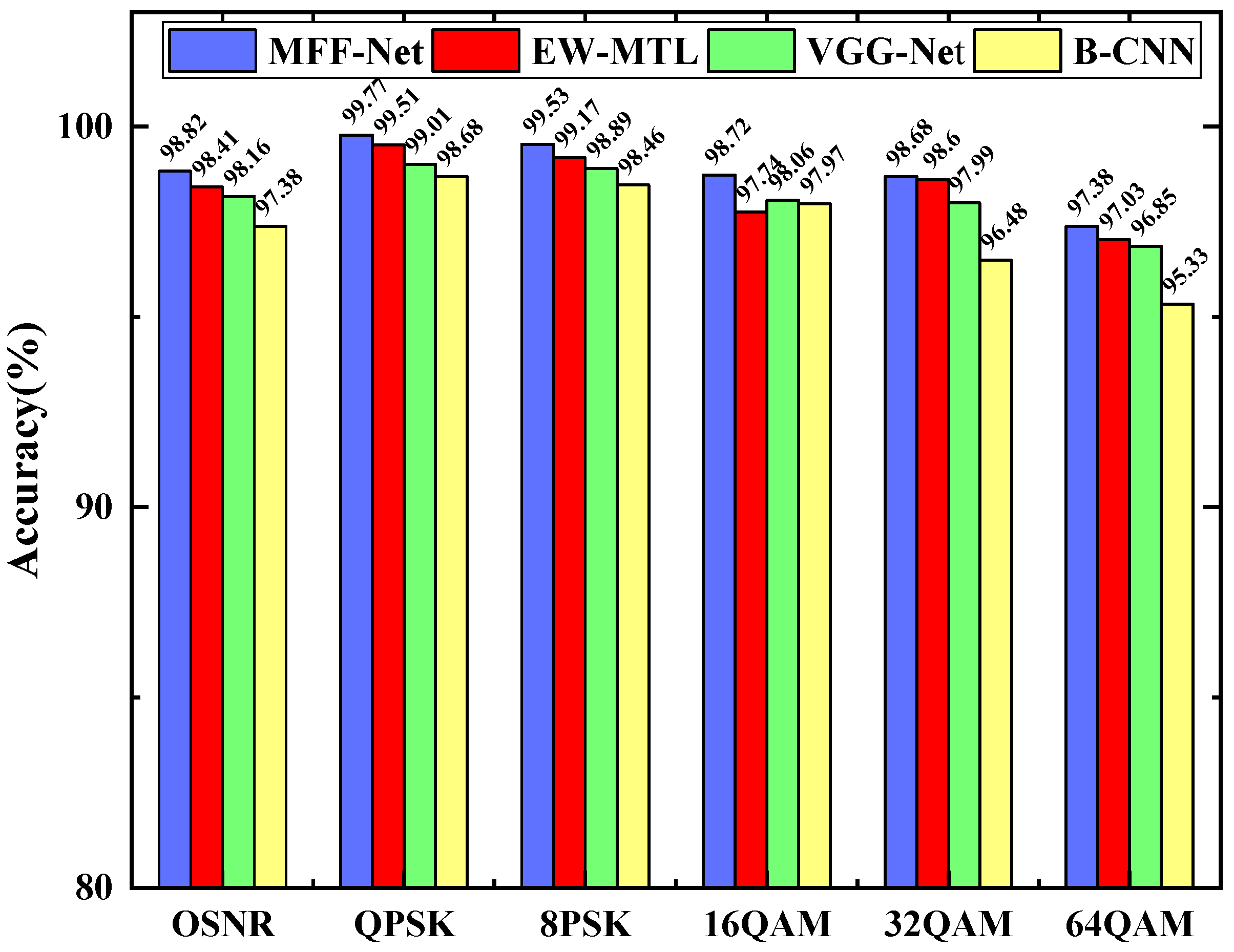
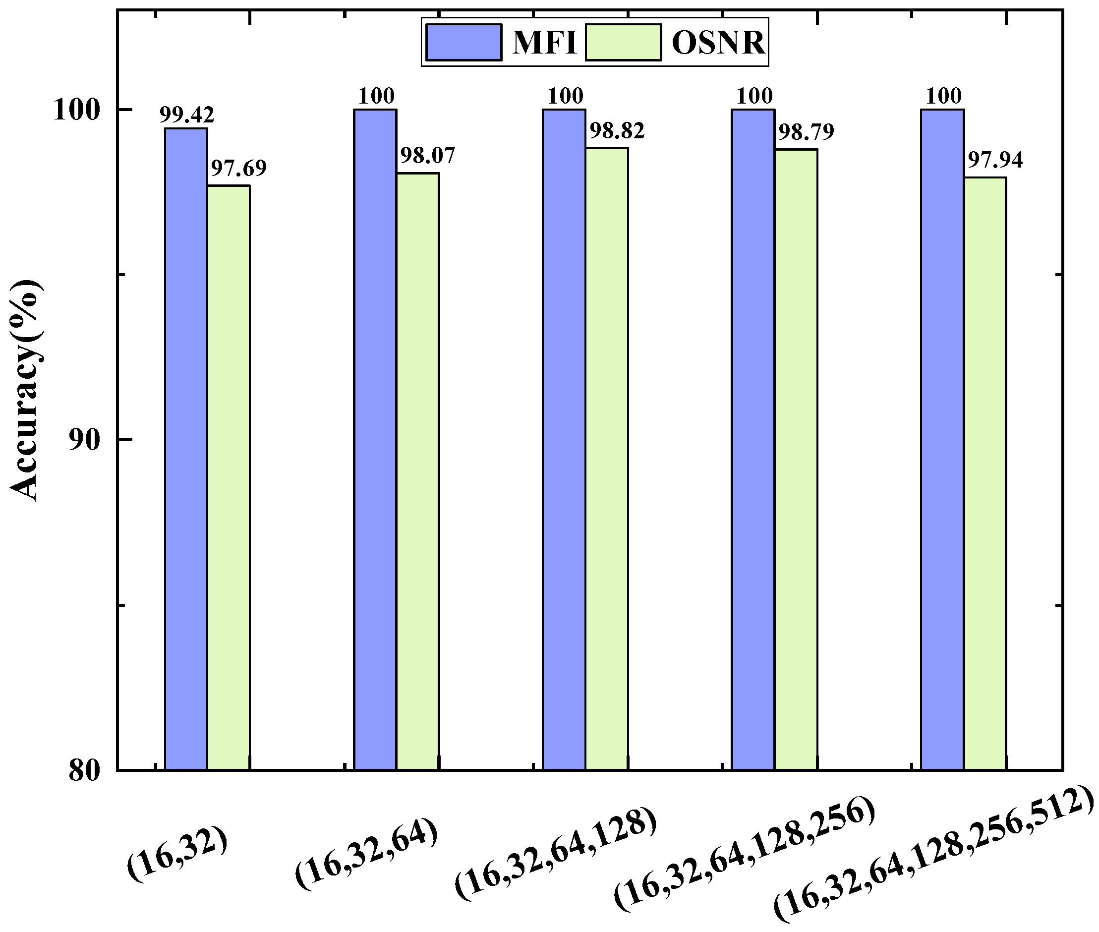
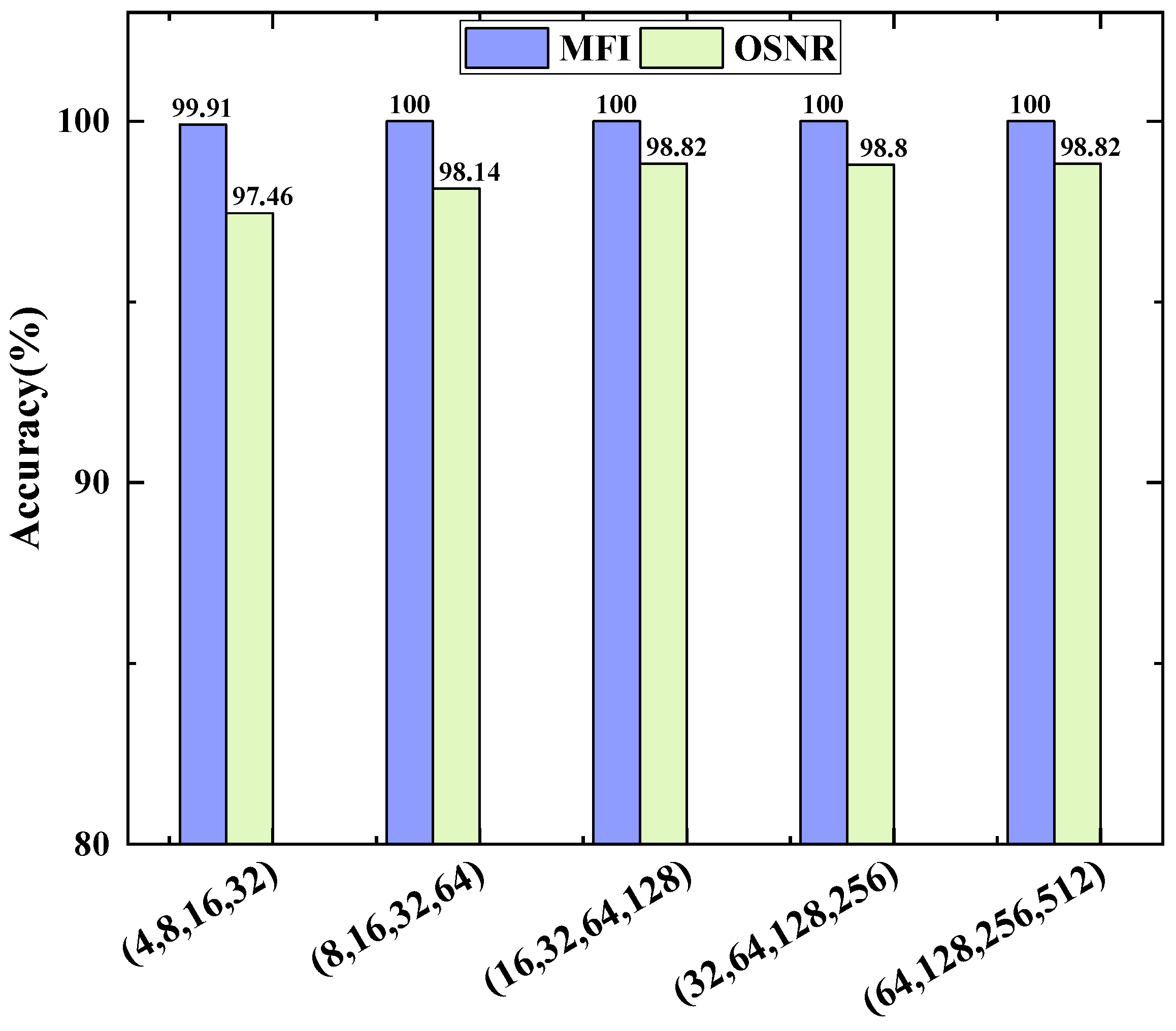
4.3. Model Structure

In this section, we analyze the effects of other factors, including the number of convolutional layers and convolutional kernels.
As demonstrated in Figure 10, the number of convolutional layers is discussed at the beginning, and (16,32), (16,32,64), (16,32,64,128), (16,32,64,128,256), (16,32,64,128,256) on the horizontal axis represent the number of convolutional layers used as 2,3,4,5, and 6, respectively. Each of these elements corresponds to the number of channels in each convolutional layer, e.g., in (16,32,64), the number of channels in the three convolutional layers is 16,32,64, respectively. Using models of different depths trained on the same dataset, the monitoring accuracy results of MFI and OSNR in Figure 10 are obtained. It can be seen that 100% MFI accuracy is achieved in all four cases except for the first. When 3 convolutional layers are applied, the monitoring precision of OSNR is 98.07%. Additionally, when there are 4 convolutional layers, the OSNR monitoring precision is 98.82%. When using 5 convolutional layers, the MFI accuracy remains the same, and the OSNR accuracy is 98.79%, which is a slight decrease. At this stage, the OSNR monitoring accuracy starts to decrease when the convolutional layers continue to be added. Therefore, we conclude that fewer convolutional layers do not bring good results, and more convolutional layers fail to achieve performance improvement and have high complexity. The structure (16,32,64,128) performs better on this dataset.
Next, we set the number of convolutional kernels from (4,8,16,32) to (64,128,256,512) and implement the change of the number of feature mappings. The accuracy curves in different cases are presented in Figure 11, with the horizontal axis being the number of feature mappings and the vertical axis indicating the accuracy of different classifications. As can be observed from the histogram, the accuracy of MFI reaches 100% in the last four situations, excluding the first one due to the too-small number of convolutional kernels. Before (16,32,64,128), OSNR monitoring accuracy increases with the number of channels. Additionally, the monitoring accuracy of OSNR reaches 98.82% at the quantity of channels per layer changes to (16,32,64,128) and no longer improves with an increase in the number of feature mappings. Again, it can be demonstrated that a more complex model structure does not lead to a better MFF-Net performance. The structure (16,32,64,128) of MFF-Net can achieve higher accuracy and lower computational complexity.

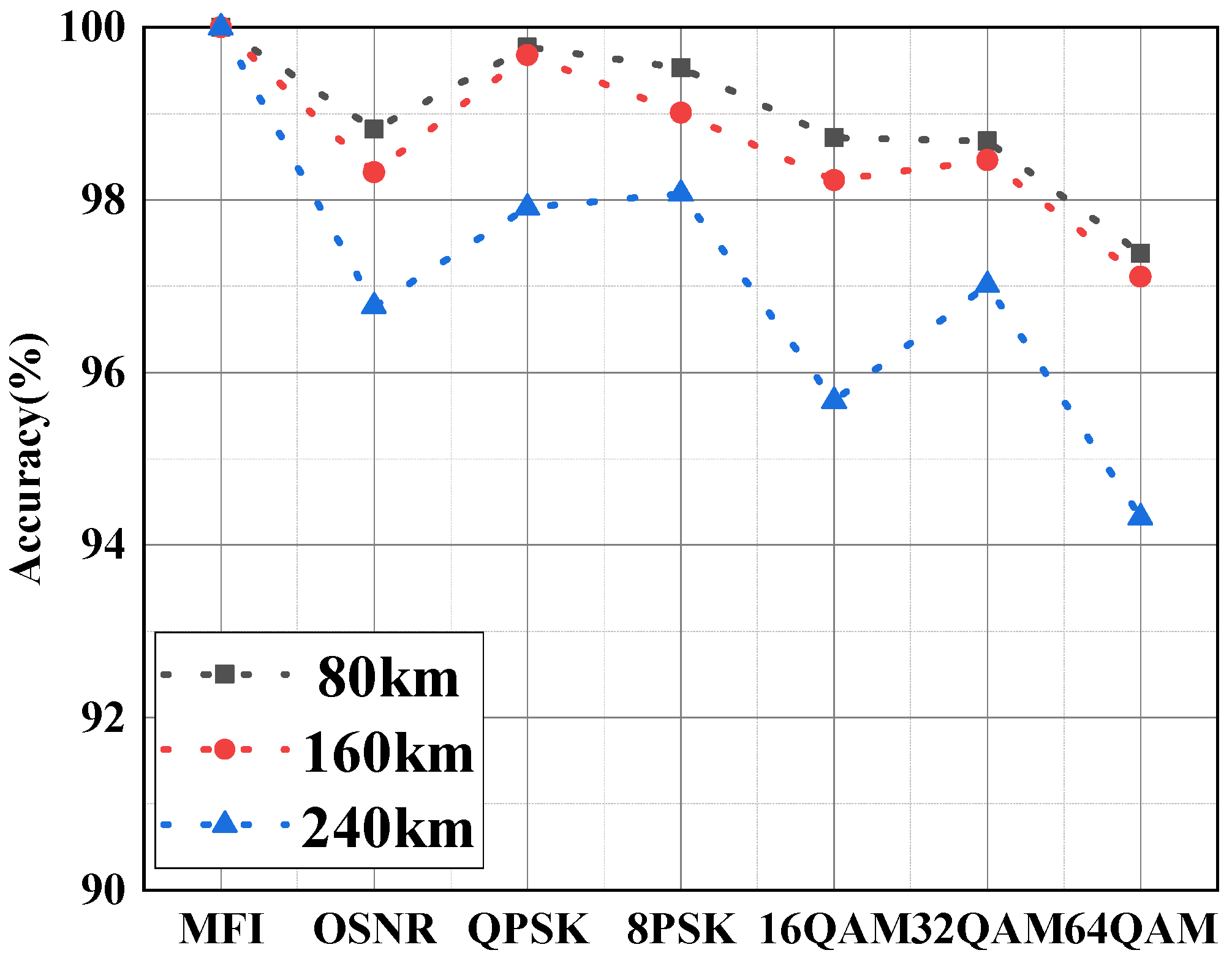
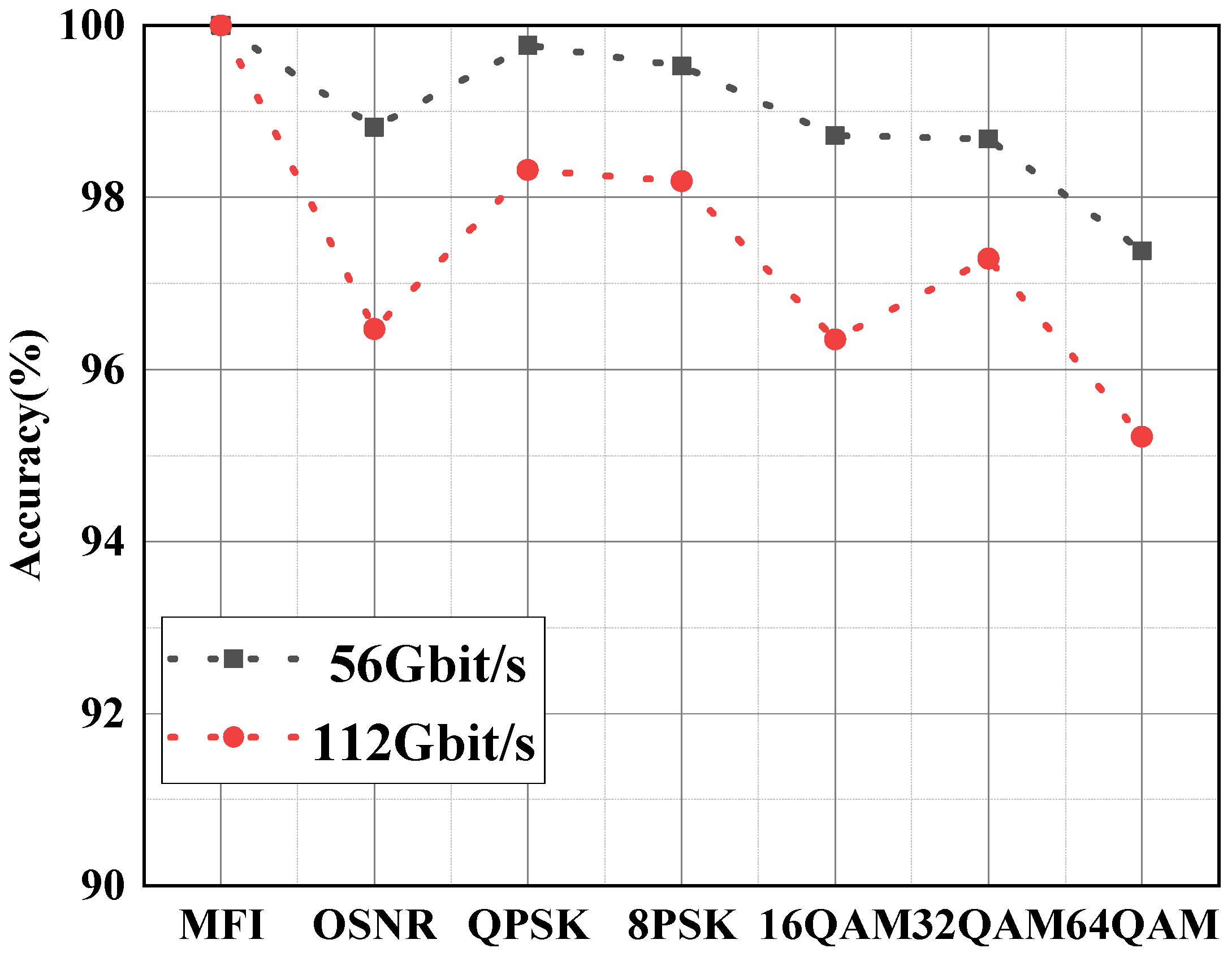
4.4. Robustness Analysis

In future optical networks with variable and complex physical parameters, it will be difficult to train models for links with fixed parameters. Therefore, we further evaluated the performance of the MFF-Net model for the QPSK/8PSK/16QAM/32QAM/64QAM simulation systems with different physical parameters.
We added transmission distances of 160 km and 240 km, keeping other parameters constant for assessing the robustness of the MFF-Net model. The simulation steps in Section 3 were repeated, and constellation maps are collected for five modulation formats. The dataset was changed to contain 3 × 11,000 = 33,000 constellation maps with three distances (80 km,160 km,240 km). The data were randomly disrupted with 70% and 30% of the training set and test set. The results of the MFF-Net model on this composite dataset are shown in Figure 12. It can be clearly seen that the MFF-Net model achieves 100% MFI accuracy based on this composite dataset. The OSNR monitoring accuracy decreases by about 1.2%. The QPSK accuracy is 98.63%, which is 1% lower than the previous single dataset. 8PSK decreases slightly. 16QAM decreases significantly by about 3%. 32QAM and 64QM decrease, respectively, by 0.7% and 0.9%.
In addition, we newly set a bit rate of 112 Gbit/s, while the rest of the parameters remained unchanged. The dataset was changed to contain 2 × 11,000 = 22,000 constellation maps, including 2 types of bit rates (56 Gbit/s, 112 Gbit/s). The data that have been randomly mixed are divided into a training set and a test set in the ratio of 7:3. We trained this dataset with the MFF-Net model, and the MFI and OSNR monitoring results are portrayed in Figure 13. Despite the increase in the number of identified states, the MFI still achieves an accuracy of 100. OSNR monitoring accuracy decreases by about 0.8%. The model proposed in this paper performs acceptably on this mixed bitrate dataset.
Although the OSNR monitoring performance of the MFF-Net model in the multi-distance and multi-bit rate systems is weakened at 97.86% and 97.97%, we have been able to derive that the MFF-Net has shown the most robustness to transmission distance and bit rate.
In addition, Figure 14 and Figure 15 show the variation in accuracy when the transmission distance increases, ranging from 80 km to 240 km, and the bit rate increases from 56 Gbit/s to 112 Gbit/s. It can also be demonstrated that the MFF-Net model is stable and robust.

5. Conclusions

In this paper, we propose a scheme based on MFF-Net for MFI and OSNR monitoring. The scheme is built on the feature extraction of fused images and achieves information complementarity between the two features. Five modulation formats (QPSK/8PSK/16QAM/32QAM/64QAM) are verified and analyzed, and 11 OSNR values are mixed at 56 Gbit/s. The correlation results indicate that the accuracy of MFI based on the MFF-Net model can reach 100%. The accuracy of OSNR monitoring is 98.82%. In addition, we conclude that MFF-Net performs better by comparing the OSNR accuracy and number of parameters of MFF-Net and B-CNN, VGG-Net and EW-MTL. Furthermore, we verified the robustness of MFF-Net by varying the transmission distance and bit rate. The proposed MFF-Net shows high performance and low complexity in this study. In the future, we can explore methods with fewer parameters to implement MFI and OSNR monitoring with high accuracy.

Author Contributions

Conceptualization, J.L. (Jingjing Li); methodology, J.L. (Jingjing Li); software, J.L. (Jingjing Li); validation, J.L. (Jingjing Li); formal analysis, J.M. and J.L. (Jianfei Liu); investigation, J.M. and J.L. (Jianfei Liu); resources, J.M. and J.L. (Jianfei Liu); data curation, J.L. (Jingjing Li); writing—original draft preparation, J.L. (Jingjing Li); writing—review and editing, J.M. and J.L. (Jianfei Liu); visualization, J.L. (Jianfei Liu) and J.L. (Jia Lu); supervision, J.L. (Jianfei Liu) and X.Z.; project administration, J.L. (Jianfei Liu); funding acquisition, J.L. (Jianfei Liu) and M.L. All authors have read and agreed to the published version of the manuscript.

Funding

This work was partially supported by the National Nature Science Foundation of China (Grant No.51077037) and the Natural Science Foundation of Hebei Province (Grant Nos.A2020202013 and F2021202054).

Institutional Review Board Statement

Not applicable.

Informed Consent Statement

Not applicable.

Data Availability Statement

Not applicable.

Conflicts of Interest

The authors declare no conflict of interest.

References

  1. Saif, W.S.; Esmail, M.A.; Ragheb, A.M.; Alshawi, T.A.; Alshebeili, S.A. Machine Learning Techniques for Optical Performance Monitoring and Modulation Format Identification: A Survey. IEEE Commun. Surv. Tutor. 2020, 22, 2839–2882. [Google Scholar] [CrossRef]
  2. Zhang, Y.; Zhou, P.; Dong, C.; Lu, Y.; Chuanqi, L. Intelligent equally weighted multi-task learning for joint OSNR monitoring and modulation format identification. Opt. Fiber Technol. 2022, 71, 102931. [Google Scholar] [CrossRef]
  3. Saif, W.S.; Ragheb, A.M.; Alshawi, T.A.; Alshebeili, S.A. Optical Performance Monitoring in Mode Division Multiplexed Optical Networks. J. Light. Technol. 2021, 39, 491–504. [Google Scholar] [CrossRef]
  4. Pan, Z.; Yu, C.; Willner, A.E. Optical performance monitoring for the next generation optical communication networks. Opt. Fiber Technol. 2010, 16, 20–45. [Google Scholar] [CrossRef]
  5. LeCun, Y.; Bengio, Y.; Hinton, G. Deep learning. Nature 2015, 521, 436–444. [Google Scholar] [CrossRef] [PubMed]
  6. Tan, S.; Mayrovouniotis, M.L. Deep learning in photonics: Introduction. Photonics Res. 2021, 9, 2327–9125. [Google Scholar]
  7. Wang, D.; Zhang, M.; Li, J.; Li, Z.; Li, J.; Song, C.; Chen, X. Intelligent constellation diagram analyzer using convolutional neural network-based deep learning. Opt. Express 2017, 25, 17150–17166. [Google Scholar] [CrossRef]
  8. Wan, Z.; Yu, Z.; Shu, L.; Zhao, Y.; Zhang, H.; Xu, K. Intelligent optical performance monitor using multi-task learning based artificial neural network. Opt. Express 2019, 27, 11281–11291. [Google Scholar] [CrossRef] [Green Version]
  9. Tanimura, T.; Hoshida, T.; Kato, T.; Watanabe, S.; Morikawa, H. Convolutional Neural Network-Based Optical Performance Monitoring for Optical Transport Networks. J. Opt. Commun. Netw. 2019, 11, A52–A59. [Google Scholar] [CrossRef]
  10. Wang, D.; Wang, M.; Zhang, M.; Zhang, Z.; Yang, H.; Li, J.; Li, J.; Chen, X. Cost-effective and data size—Adaptive OPM at intermediated node using convolutional neural network-based image processor. Opt. Express 2019, 27, 9403–9419. [Google Scholar] [CrossRef]
  11. Yu, Z.; Wan, Z.; Shu, L.; Hu, S.; Zhao, Y.; Zhang, J.; Xu, K. Loss weight adaptive multi-task learning based optical performance monitor for multiple parameters estimation. Opt. Express 2019, 27, 37041–37055. [Google Scholar] [CrossRef] [PubMed]
  12. Khan, F.N.; Zhong, K.; Zhou, X.; Al-Arashi, W.H.; Yu, C.; Lu, C.; Lau, A.P.T. Joint OSNR monitoring and modulation format identification in digital coherent receivers using deep neural networks. Opt. Express 2017, 25, 17767–17776. [Google Scholar] [CrossRef]
  13. Zheng, J.; Lv, Y. Likelihood-Based Automatic Modulation Classification in OFDM with Index Modulation. IEEE Trans. Veh. Technol. 2018, 67, 8192–8204. [Google Scholar] [CrossRef]
  14. Lin, X.; Eldemerdash, Y.A.; Dobre, O.A.; Zhang, S.; Li, C. Modulation Classification Using Received Signal’s Amplitude Distribution for Coherent Receivers. IEEE Photonics Technol. Lett. 2017, 29, 1872–1875. [Google Scholar] [CrossRef] [Green Version]
  15. Liu, G.; Proietti, R.; Zhang, K.; Lu, H.; Yoo, S.B. Blind modulation format identification using nonlinear power transformation. Opt. Express 2017, 25, 30895–30904. [Google Scholar] [CrossRef] [PubMed]
  16. Yi, A.; Liu, H.; Yan, L.; Jiang, L.; Pan, Y.; Luo, B. Amplitude variance and 4th power transformation based modulation format identification for digital coherent receiver. Opt. Commun. 2019, 452, 109–115. [Google Scholar] [CrossRef]
  17. Khan, F.N.; Zhou, Y.; Lau, P.T.A.; Lu, C. Modulation format identification in heterogeneous fiber-optic networks using artificial neural networks. Opt. Express 2012, 20, 12422–12431. [Google Scholar] [CrossRef] [PubMed] [Green Version]
  18. Wang, D.; Zhang, M.; Li, Z.; Li, J.; Fu, M.; Cui, Y.; Chen, X. Modulation Format Recognition and OSNR Estimation Using CNN-Based Deep Learning. IEEE Photonics Technol. Lett. 2017, 29, 1667–1670. [Google Scholar] [CrossRef]
  19. Wang, Z.; Yang, A.; Guo, P.; He, P. OSNR and nonlinear noise power estimation for optical fiber communication systems using LSTM based deep learning technique. Opt. Express 2018, 26, 21346–21357. [Google Scholar] [CrossRef]
  20. Wang, C.; Fu, S.; Wu, H.; Luo, M.; Li, X.; Tang, M.; Liu, D. Joint OSNR and CD monitoring in digital coherent receiver using long short-term memory neural network. Opt. Express 2019, 27, 6936–6945. [Google Scholar] [CrossRef]
  21. Xia, L.; Zhang, J.; Hu, S.; Zhu, M.; Song, Y.; Qiu, K. Transfer learning assisted deep neural network for OSNR estimation. Opt. Express 2019, 27, 19398–19406. [Google Scholar] [CrossRef]
  22. Zhang, J.; Gao, M.; Ma, Y.; Zhao, Y.; Chen, W.; Shen, G. Intelligent adaptive coherent optical receiver based on convolutional neural network and clustering algorithm. Opt. Express 2018, 26, 18684–18698. [Google Scholar] [CrossRef] [PubMed]
  23. Eltaieb, R.A.; Farghal, A.E.A.; Ahmed, H.E.-D.H.; Saif, W.S.; Ragheb, A.M.; Alshebeili, S.A.; Shalaby, H.M.H.; El-Samie, F.E.A. Efficient Classification of Optical Modulation Formats Based on Singular Value Decomposition and Radon Transformation. J. Light. Technol. 2019, 38, 619–631. [Google Scholar] [CrossRef]
  24. Zhang, W.; Zhu, D.; Zhang, N.; Xu, H.; Zhang, X.; Zhang, H.; Li, Y. Identifying Probabilistically Shaped Modulation Formats Through 2D Stokes Planes With Two-Stage Deep Neural Networks. IEEE Access 2020, 8, 6742–6750. [Google Scholar] [CrossRef]
  25. Shen, F.; Zhou, J.; Huang, Z.; Li, L. Going Deeper into OSNR Estimation with CNN. Photonics 2021, 8, 402. [Google Scholar] [CrossRef]
  26. Yang, L.; Xu, H.; Bai, C.; Yu, X.; You, K.; Sun, W.; Guo, J.; Zhang, X.; Liu, C. Modulation Format Identification Using Graph-Based 2D Stokes Plane Analysis for Elastic Optical Network. IEEE Photonics J. 2021, 13, 7901315. [Google Scholar] [CrossRef]
  27. Chen, X.; Li, Y.; Li, Y. Multi-feature fusion point cloud completion network. World Wide Web 2021, 25, 1551–1564. [Google Scholar] [CrossRef]
  28. Zhang, Z.; Li, X.; Gan, C. Multimodality Fusion for Node Classification in D2D Communications. IEEE Access 2018, 6, 63748–63756. [Google Scholar] [CrossRef]
  29. Zhao, Y.; Yu, Z.; Wan, Z.; Hu, S.; Shu, L.; Zhang, J.; Xu, K. Low Complexity OSNR Monitoring and Modulation Format Identification Based on Binarized Neural Networks. J. Light. Technol. 2020, 38, 1314–1322. [Google Scholar] [CrossRef]
  30. Lv, H.; Zhou, X.; Huo, J.; Yuan, J. Joint OSNR monitoring and modulation format identification on signal amplitude histograms using convolutional neural network. Opt. Fiber Technol. 2021, 61, 102455. [Google Scholar] [CrossRef]
  31. Xie, Y.; Wang, Y.; Kandeepan, S.; Wang, K. Machine Learning Applications for Short Reach Optical Communication. Photonics 2022, 9, 30. [Google Scholar] [CrossRef]
Figure 1. Samples of the constellation and horizontal projection for all modulation formats at OSNR = 25 dB. (a) QPSK, (b) 8PSK, (c) 16QAM, (d) 32QAM, and (e) 64QAM.
Photonics 10 00373 g001
Figure 2. Schematic diagram of the structure for the MFF-Net model.
Photonics 10 00373 g002
Figure 3. Feature Fusion Module.
Photonics 10 00373 g003
Figure 4. Simulation setup of the coherent optical communication system. PRBS, pseudo-random binary sequence; CW laser, continuous wave laser; Dual MZM, dual Mach–Zehnder modulator; OA, optical amplifier; LO, local oscillator.
Photonics 10 00373 g004
Figure 5. The MFI accuracies at different epochs for different models.
Photonics 10 00373 g005
Figure 6. The MFI accuracies at different epochs for different sample numbers. The sample numbers of each format are 550, 1100, and 2200.
Photonics 10 00373 g006
Figure 7. OSNR monitoring accuracy at different epochs.
Photonics 10 00373 g007
Figure 8. OSNR monitoring accuracy between MFF-Net and the other three algorithms.
Photonics 10 00373 g008
Figure 9. Comparison of OSNR monitoring accuracy curves for different modulation formats.
Photonics 10 00373 g009
Figure 10. MFI and OSNR accuracies for different numbers of convolutional layers.
Photonics 10 00373 g010
Figure 11. MFI and OSNR accuracies for different numbers of convolutional kernels.
Photonics 10 00373 g011
Figure 12. Accuracies for MFF-Net trained on data from three different transmission distances (80 km, 160 km, and 240 km).
Photonics 10 00373 g012
Figure 13. Accuracies for MFF-Net trained on data from two different bitrates (56 Gbit/s, 112 Gbit/s).
Photonics 10 00373 g013
Figure 14. Accuracies for MFF-Net trained on data from 80 km, 160 km, and 240 km.
Photonics 10 00373 g014
Figure 15. Accuracies for MFF-Net trained on data from 56 Gbit/s and 112 Gbit/s.
Photonics 10 00373 g015
Table 1. Comparison of different models.
Model TypeMFF-NetB-CNNVGG-NetEW-MTLCNNLSTM
OSNR
Accuracy
98.82%97.38%98.16%98.41%97.13%95.53%
Total
Parameters
2.64 × 1051.63 × 1084.27 × 1064.76 × 1052.51 × 1064.80 × 105
Disclaimer/Publisher’s Note: The statements, opinions and data contained in all publications are solely those of the individual author(s) and contributor(s) and not of MDPI and/or the editor(s). MDPI and/or the editor(s) disclaim responsibility for any injury to people or property resulting from any ideas, methods, instructions or products referred to in the content.

