Mach–Zehnder Modulator Output in Time and Frequency Domain—Calculation and Experimental Confirmation

Abstract

The Mach–Zehnder intensity Modulator (MZM), named after Ludwig Mach and Ludwig Zehnder, is based on the corresponding interferometer. It splits light into two counter-rotating partial beams, which are later recombined with a controlled phase difference. The output of the MZM depends on the phase difference of the interferometer paths. This phase difference is usually adjusted by an electrical voltage applied to a Phase Shifter (PS) placed in one of the interferometer arms. For MZM applications in which the wavelength is changing, the applied voltage must be adjusted accordingly. We derived the equations describing the MZM output in the frequency domain for the case of a triangular PS voltage (necessary for a sinusoidal output) and compared the analytical results with measurements. Our setup uses an Optical Parametric Oscillator (OPO) with a tunable wavelength from 3.2–3.5 μm as the light source and a Lithium Tantalate (LT)-PS for the MZM’s phase modulation. The novel insights enable new control methods for MZMs particularly suited for spectroscopic applications where the wavelength is scanned or otherwise altered.

1. Introduction

The Mach–Zehnder intensity Modulator (MZM) is widely used for the intensity modulation of optical signals, for example, in fiber-optic communication [1]. It has also gained significant importance as an electro-optic modulator for spectroscopic applications, e.g., Photoacoustic Spectroscopy (PAS). PAS is a powerful technique for studying the interaction of light with matter, with applications in a range of fields, including environmental monitoring, biomedical imaging, and materials science [2,3].

In particular, PAS requires modulated radiation to excite the sample in a way that an acoustic signal is generated [4]. High-frequency stability is very important in this application because the acoustic detection module usually acts as a band-pass filter and hence cuts off signals outside the band-pass width. Compared to the mechanical chopper, a MZM can provide a pure sinusoidal signal free of mechanical influences, which leads to an improvement in precision and stability. Another key advantage of MZMs is their ability to provide high modulation frequencies.

In MZMs, the modulation occurs as a result of the interference of two partial beams of different phases. The difference in phase depends on several factors but can be adjusted using a voltage applied to the MZM’s Phase Shifter (PS). Effects on the modulation by temperature, displacement, and wavelength variation can be observed in the interference and hence in the optical signal. A systematic control of the MZM can oppose these effects. According to the state of the art, the bias voltage control of the modulator is performed by monitoring the power of the output signal and adjusting the bias voltage to match the MZM operation point [5]. A different approach is to monitor the harmonics of the output signal instead of its power [6]. A bias voltage is the Direct Current (DC) component of the PS’s control voltage. Furthermore, there are first approaches to model-based controls [7].

The aim of this investigation is to evaluate a mathematical model of the characteristics of the interfering optical signal in the frequency domain. This novel approach could lead to an inclusion of the wavelength dependency directly in a control algorithm and thus enable more efficient control of the MZM.

The paper is structured as follows: Section 2 describes our experimental setup, followed by the MZM fundamentals and its operating parameters in Section 3. The novel calculation of the MZM output signal in the frequency domain is presented in Section 4. Section 5 includes a comparison of the experimental and analytical results, concluded by a discussion in Section 6.

2. Experimental Setup

The MZM is part of a PAS setup measuring Volatile Organic Compounds (VOCs) in air [8]. Since the VOCs have broadband absorption spectra, we use an Optical Parametric Oscillator (OPO), type Argos, model 2400-BB-5 Module C from Lockheed Martin Aculight in Bothell, WA, USA, with a tunable wavelength of 3.2–3.5 μm as a light source. The pump laser is a high-power diode-pumped ytterbium fiber laser, model YLR-10-1064-LP-SF from IPG Photonics in Oxford, MA, USA.

The free-beam MZM used in our experimental setup is a self-construction and uses a Lithium Tantalate (LT)-PS model PS3T-MWIR1 from QUBIG in Munich, Germany, two beam splitters, type BSW510 from Thorlabs Inc. Newton, New Jersey, and two protected silver mirrors type PF10-03-P01, from Thorlabs. The LT crystal is coated with a broadband anti-reflection coating that reduces reflections in the wavelength range from 3–4.5 μm to less than 1%. Floating electrodes allow differential voltage operation. The PS’s voltage is controlled with a function generator, model 33220A from Agilent Technologies in Santa Clara, CA, USA and a high voltage linear amplifier including internal DC bias source, model HVA-A075-D1.5 from QUBIG ($V_{\mathrm{AC}}=$ 0–0.75 kV and $V_{\mathrm{DC}}=$ 0–1.5 kV).

To detect the MZM’s transmission, an InAsSb fixed gain amplified detector, model PDA07P2 from Thorlabs with a range from 2.7 μm to 5.3 μm is used. The detector’s transimpedance gain at Hi-Z is 300 $\mathrm{k}$$\mathrm{V}$${\mathrm{A}}^{-1}$. It is used at constant room temperature of 19 ${}^{\circ }\mathrm{C}$ and wavelength of 3.4 μm, the sensor’s responsivity at these conditions equals $(4.7\pm 0.2)$ $\mathrm{m}$$\mathrm{A}$${\mathrm{W}}^{-1}$. 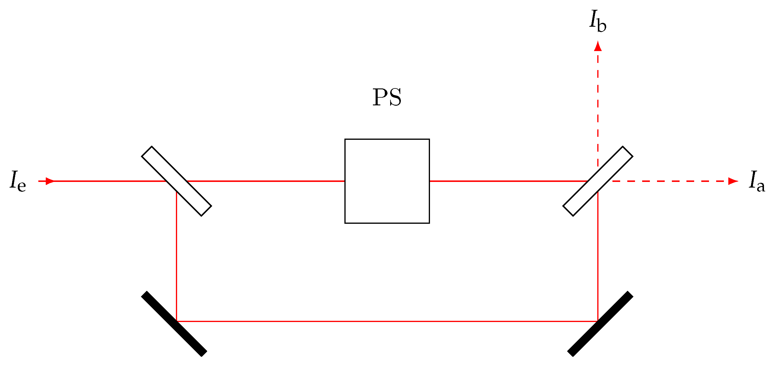This leads to an amplification of $(1.41\pm 0.06)$ $\mathrm{V} \mathrm{m}{\mathrm{W}}^{-1}$ at the detector’s output. The signal is then processed by a data acquisition card, model USB-6210 from National Instruments in Austin, TX. A schematic of the MZM’s setup is shown in Figure 1.

3. Mach–Zehnder Intensity Modulator Fundamentals

The MZM is based on the alternation between constructive and destructive interference. The interference is generated as follows: A beam splitter divides incident light into two beams of approximately the same intensity. After passing through two different optical paths, with the PS in one of them, the beams are superimposed using a second beam splitter.

The input beam has the intensity $I_{\mathrm{e}}$, and the output beams have the intensities $I_{\mathrm{a}}$ and $I_{\mathrm{b}}$, respectively. The relationship between output and input intensity $I_{\mathrm{a},\mathrm{b}}/I_{\mathrm{e}}$ can be described as transmission ${\tau }_{\mathrm{a},\mathrm{b}}$, which is a function of the phase difference $\varphi$ between the two counter-rotating partial beams [1]

$$\begin{array}{cc}\hfill {\tau }_{\mathrm{a}}& ={cos}^2\left(\frac{\varphi }{2}\right),\hfill \end{array}$$

(1a)

$$\begin{array}{cc}\hfill {\tau }_{\mathrm{a}}& =\frac{1+cos\left(\varphi \right)}{2}.\hfill \end{array}$$

(1b)

Equation (1b) is an alternative variant of the commonly used Equation (1a), which allows us to convert the output signal easier into the frequency domain. The corresponding transmission ${\tau }_{\mathrm{b}}$ can be calculated analogously by replacing $\varphi$ with $\varphi +\pi$.

By changing the voltage $V\left(t\right)$ applied to the PS, $\varphi$ and the corresponding transmission ${\tau }_{\mathrm{a},\mathrm{b}}$ can be adjusted due to the Pockels effect [1]

$$\varphi = \pi \frac{V\left(t\right)}{V_{\lambda /2}}+C.$$

(2)

The half-wave voltage $V_{\lambda /2}$ is the voltage required to shift the phase $\varphi$ by $\pi$. It is material and wavelength dependent. For the transverse Pockels effect, the voltage is applied perpendicular to the optical axis. The half-wave voltage is a function of the electrode distance $d_{\mathrm{PS}}$ and the crystal length $l_{\mathrm{PS}}$

$$V_{\lambda /2}=\frac{\lambda }{n_{\mathrm{e}}^3{r}_{33}}\frac{d_{\mathrm{PS}}}{l_{\mathrm{PS}}}.$$

(3)

Here, $r_{33}$ is the electro-optic coefficient and $n_{\mathrm{e}}$ the extraordinary refractive index of LT [9,10].

Besides the intentional modulation by $V\left(t\right)$, the phase depends on semi-constant factors like the difference in optical path length and the PS’s temperature, summarized as C. One of these factors is the voltage free phase shift ${\varphi }_{\mathrm{PS}}\in C$ of the PS, calculated using Equation (4a) [10]. Another factor is the inequality of the optical length $l_{\mathrm{imb}}$ of the MZM in combination with temperature and wavelength fluctuations. For imbalanced MZMs, the phase ${\varphi }_{\mathrm{imb}}\in C$ of the Mach–Zehnder interferometer is calculated using Equation (4b) [11,12]

$$\begin{array}{cc}\hfill {\varphi }_{\mathrm{PS}}& =\frac{2\pi n_{\mathrm{e}}{l}_{\mathrm{PS}}}{\lambda },\hfill \end{array}$$

(4a)

$$\begin{array}{cc}\hfill {\varphi }_{\mathrm{imb}}& =\frac{2\pi n_{\mathrm{air}}{l}_{\mathrm{imb}}}{\lambda },\hfill \end{array}$$

(4b)

with the refractive index of air $n_{\mathrm{air}}$, the optical length inequality $l_{\mathrm{imb}}$ between the two arms of the MZM, and the wavelength $\lambda$ of the OPO.

4. Calculation of MZM Output Signal

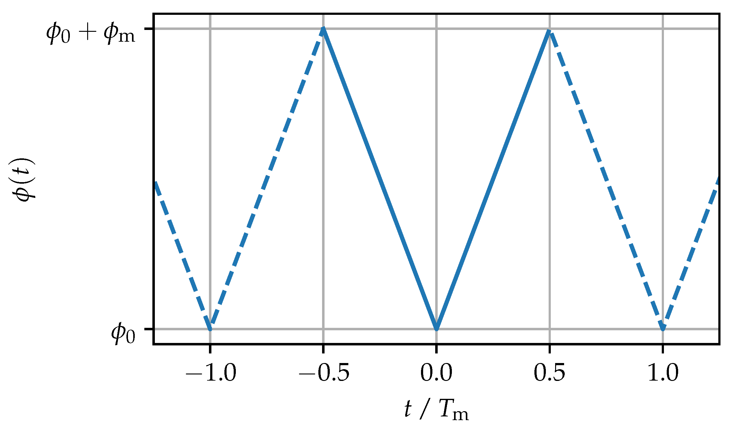
The transmission of the MZM is a function of ${cos}^2$ of $\varphi$ (see Equation (1a,b); therefore, a triangular phase modulation of the PS is required to obtain a pure sinusoidal output signal. Since voltage and phase of the PS are proportional (see Equation (2)), the voltage modulation of the PS needs to be triangular as well. In Figure 2 the modulated phase $\varphi \left(t\right)$ of the PS is shown.

The triangular voltage and phase modulation $\varphi$ can be described as

$$\begin{array}{cc}\hfill \varphi \left(t\right)& ={\varphi }_0+\left|2{\varphi }_{\mathrm{m}}{f}_{\mathrm{m}}t\right|\mathrm{for}-T_{\mathrm{m}}/2\le t<T_{\mathrm{m}}/2,\mathrm{or}\hfill \end{array}$$

(5a)

$$\begin{array}{cc}\hfill \varphi \left(t\right)& =\left\{\begin{array}{cc}{\varphi }_0-2{\varphi }_{\mathrm{m}}{f}_{\mathrm{m}}t\hfill & \mathrm{for}-T_{\mathrm{m}}/2\le t<0,\hfill \\ {\varphi }_0+2{\varphi }_{\mathrm{m}}{f}_{\mathrm{m}}t\hfill & \mathrm{for}\phantom{-T/2}0\le t<T_{\mathrm{m}}/2,\hfill \end{array}\right.\hfill \end{array}$$

(5b)

with the modulation frequency $f_{\mathrm{m}}$ and its period $T_{\mathrm{m}}=1/f_{\mathrm{m}}$. The modulated phase ${\varphi }_{\mathrm{m}}$ depends on the peak-to-peak amplitude of the triangular voltage $V_{\mathrm{m}}$ (see Equation (6a)), the phase ${\varphi }_0$ depends on the voltage offset $V_0$

$$\begin{array}{cc}\hfill {\varphi }_{\mathrm{m}}& =\pi V_{\mathrm{m}}/V_{\lambda /2},\hfill \end{array}$$

(6a)

$$\begin{array}{cc}\hfill {\varphi }_0& =\pi V_0/V_{\lambda /2}+C.\hfill \end{array}$$

(6b)

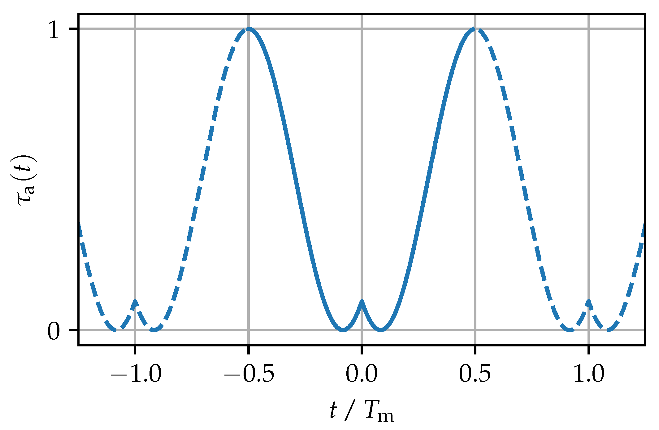
C stands for the voltage independent factors introduced in Equation (2). A resulting exemplary transmission according to Equations (1a) and (5a,b) with ${\varphi }_0=0.8\pi$ and ${\varphi }_{\mathrm{m}}=1.2\pi$ is shown in Figure 3.

The transmission will be purely sinusoidal as long as $\varphi \left(t\right)$ represents a linear sweep. Since the function is not differentiable (its derivative is not continuous), harmonics arise, which is undesirable in many applications. These harmonics will be further analyzed in the following.

We consider the phase-dependent cosine component of Equation (1b) as the signal

$$s=cos\left(\varphi \right)$$

(7)

and assume this signal to be extended periodically for all time. This aspect will become important for the calculation of the resulting spectrum. Combining the triangular phase from Equation (5b) with the signal from Equation (7) and taking advantage of the fact that $cos\left(x\right)=cos(-x)$ leads to

$$s\left(t\right)=cos(2{\varphi }_{\mathrm{m}}{f}_{\mathrm{m}}t+{\varphi }_0)·rect\left(\frac{t-T_{\mathrm{m}}/4}{T_{\mathrm{m}}/2}\right)+cos(2{\varphi }_{\mathrm{m}}{f}_{\mathrm{m}}t-{\varphi }_0)·rect\left(\frac{t+T_{\mathrm{m}}/4}{T_{\mathrm{m}}/2}\right).$$

(8)

Hereby, the shifted rectangular function serves as a window function of width $T_{\mathrm{m}}/2$ to translate the section-wise defined phase into an easy-to-transform mathematical form. It is centered at $\pm T_{\mathrm{m}}/4$ and, thus, incorporates the sign difference shown in Equation (5b) at negative and positive time. By applying a Fourier transform, we can calculate the complex spectrum $\underline{S}\left(f\right)$ of the signal.

$$\begin{array}{c}\underline{S}\left(f\right)=\frac{1}{2}\left[\delta \left(f-\frac{{\varphi }_{\mathrm{m}}{f}_{\mathrm{m}}}{\pi }\right)e^{\mathrm{j}{\varphi }_0}+\delta \left(f+\frac{{\varphi }_{\mathrm{m}}{f}_{\mathrm{m}}}{\pi }\right)e^{-\mathrm{j}{\varphi }_0}\right]\ast \frac{T_{\mathrm{m}}}{2}sinc\left(\frac{\pi f{T}_{\mathrm{m}}}{2}\right)e^{-\mathrm{j}\pi f{T}_{\mathrm{m}}/2}\hfill \\ +\frac{1}{2}\left[\delta \left(f-\frac{{\varphi }_{\mathrm{m}}{f}_{\mathrm{m}}}{\pi }\right)e^{-\mathrm{j}{\varphi }_0}+\delta \left(f+\frac{{\varphi }_{\mathrm{m}}{f}_{\mathrm{m}}}{\pi }\right)e^{\mathrm{j}{\varphi }_0}\right]\ast \frac{T_{\mathrm{m}}}{2}sinc\left(\frac{\pi f{T}_{\mathrm{m}}}{2}\right)e^{\mathrm{j}\pi f{T}_{\mathrm{m}}/2}\\ \hfill +s_{\mathrm{DC}}({\varphi }_{\mathrm{m}},{\varphi }_0)\delta \left(f\right)\ast T_{\mathrm{m}}sinc\left(\pi f{T}_{\mathrm{m}}\right).\end{array}$$

(9)

In the above equation, the sinus cardinalis function is used in its unnormalized form $sinc\left(x\right)=sin\left(x\right)/x$ and $\delta \left(x\right)$ refers to the Dirac delta distribution

$$\delta \left(x\right)=\left\{\begin{array}{cc}\infty \hfill & \mathrm{for}x=0,\hfill \\ 0\hfill & \mathrm{for}x\ne 0,\hfill \end{array}\right.$$

(10)

with a constraint to satisfy ${\int }_{-\infty }^{\infty }\delta \left(x\right)\mathrm{d}x=1$. The ∗ operator represents the convolution of the two functions. The term $s_{\mathrm{DC}}({\varphi }_{\mathrm{m}},{\varphi }_0)$ represents a possible DC part of $s\left(t\right)$. This part is dependent on ${\varphi }_{\mathrm{m}}$ and ${\varphi }_0$ but independent of time. As $s\left(t\right)$ is symmetric with respect to the y-axis, we can calculate it to be

$$\begin{array}{cc}\hfill s_{\mathrm{DC}}& =\frac{2}{T_{\mathrm{m}}}{\int }_0^{T_{\mathrm{m}}/2}s\left(t\right)\mathrm{d}t\hfill \end{array}$$

(11a)

$$\begin{array}{cc}\hfill & \hspace{1em}\hspace{1em}\hspace{1em}\hspace{1em} =\frac{2}{T_{\mathrm{m}}}{\int }_0^{T_{\mathrm{m}}/2}cos(2{\varphi }_{\mathrm{m}}{f}_{\mathrm{m}}t+{\varphi }_0)\mathrm{d}t\hfill \end{array}$$

(11b)

$$\begin{array}{cc}\hfill & \hspace{1em}\hspace{1em}\hspace{1em}\hspace{1em} =\frac{2}{T_{\mathrm{m}}}\frac{sin(2{\varphi }_{\mathrm{m}}{f}_{\mathrm{m}}t+{\varphi }_0)}{2{\varphi }_{\mathrm{m}}{f}_{\mathrm{m}}}{|}_0^{T_{\mathrm{m}}/2}\hfill \end{array}$$

(11c)

$$\begin{array}{cc}\hfill & \hspace{1em}\hspace{1em}\hspace{1em}\hspace{1em} =\frac{sin({\varphi }_{\mathrm{m}}+{\varphi }_0)-sin\left({\varphi }_0\right)}{{\varphi }_{\mathrm{m}}}.\hfill \end{array}$$

(11d)

The expression for $\underline{S}\left(f\right)$ in Equation (9) can be simplified using the properties of the convolution with a Dirac function (Equation (10)) as well as rearranging the phase shifts. The result is a purely real spectrum

$$\begin{array}{c}S\left(f\right)=\frac{T_{\mathrm{m}}}{2}\left[sinc\left(\frac{\pi f{T}_{\mathrm{m}}-{\varphi }_{\mathrm{m}}}{2}\right)cos\left({\varphi }_0-\frac{\pi f{T}_{\mathrm{m}}-{\varphi }_{\mathrm{m}}}{2}\right)\right.\hfill \\ \hspace{1em}\hspace{1em}\hspace{1em}\hspace{1em}\hspace{1em}\hspace{1em}\hspace{1em}+\left.sinc\left(\frac{\pi f{T}_{\mathrm{m}}+{\varphi }_{\mathrm{m}}}{2}\right)cos\left({\varphi }_0+\frac{\pi f{T}_{\mathrm{m}}+{\varphi }_{\mathrm{m}}}{2}\right)\right]\\ \hspace{1em}\hspace{1em}\hspace{1em}\hspace{1em}\hspace{1em}\hspace{1em}\hspace{1em}\hspace{1em}\hspace{1em}\hspace{1em}\hspace{1em}\hspace{1em}\hspace{1em}\hspace{1em}\hspace{1em}\hspace{1em}\hspace{1em}\hspace{1em}\hspace{1em}\hspace{1em}\hspace{1em}\hspace{1em}\hspace{1em}\hspace{1em}+s_{\mathrm{DC}}{T}_{\mathrm{m}}sinc\left(\pi f{T}_{\mathrm{m}}\right).\end{array}$$

(12)

The interim steps to get from Equation (9) to (12) can be found in Appendix A.

Periodical repetition of our signal leads to a discrete spectrum $S_{\mathrm{p}}\left(f\right)$. This discrete spectrum is only defined at multiples of the fundamental frequency $f=k{f}_{\mathrm{m}}$ with $k\in \mathbb{N}$. Additionally, we get a factor of $1/T_{\mathrm{m}}$ in the spectrum by changing our description of the signal to a periodical form. Depending on ${\varphi }_{\mathrm{m}}$, the resulting spectrum can be at the peak of the sinc function or also on side slopes

$$\begin{array}{c}{S}_{\mathrm{p}}\left(f\right)=\sum _{k=-\infty }^{\infty }\delta (f-k{f}_{\mathrm{m}})\left[\frac{1}{2}sinc\left(\frac{\pi k-{\varphi }_{\mathrm{m}}}{2}\right)cos\left({\varphi }_0-\frac{\pi k-{\varphi }_{\mathrm{m}}}{2}\right)\right.\hfill \\ \hspace{1em}\hspace{1em}\hspace{1em}\hspace{1em}\hspace{1em}\hspace{1em}\hspace{1em}\hspace{1em}+\left.\frac{1}{2}sinc\left(\frac{\pi k+{\varphi }_{\mathrm{m}}}{2}\right)cos\left({\varphi }_0+\frac{\pi k+{\varphi }_{\mathrm{m}}}{2}\right)+s_{\mathrm{DC}}sinc\left(\pi k\right)\right].\end{array}$$

(13)

The final result is a purely real, discrete, and symmetric spectrum. In Figure 4, the amplitude spectrum (frequency domain) of the previous example in Figure 3 (time domain) is shown. The amplitude spectrum at each valid frequency $f=k{f}_{\mathrm{m}}$ can easily be calculated by taking the absolute value of the expression in the square brackets with the following k. All other frequencies have, per the definition of periodicity, an amplitude of 0. The solid green line in Figure 4 corresponds to the absolute value of the spectrum $\left|S\right(f\left)\right|$, normalized by $T_{\mathrm{m}}$, and the blue stems are the absolute value of the end result when the signal is periodically extended $|S_{\mathrm{p}}\left(f\right)|$. We have additionally plotted the three summands of Equation (12) separately: the left shifted sinc function $B=0.5T_{\mathrm{m}}sinc\left((\pi f{T}_{\mathrm{m}}+{\varphi }_{\mathrm{m}})/2\right)cos\left({\varphi }_0+(\pi f{T}_{\mathrm{m}}+{\varphi }_{\mathrm{m}})/2\right)$, the right shifted sinc function $C=0.5T_{\mathrm{m}}sinc\left((\pi f{T}_{\mathrm{m}}-{\varphi }_{\mathrm{m}})/2\right)cos\left({\varphi }_0-(\pi f{T}_{\mathrm{m}}-{\varphi }_{\mathrm{m}})/2\right)$ as well as the DC part $A=s_{\mathrm{DC}}{T}_{\mathrm{m}}sinc\left(\pi f{T}_{\mathrm{m}}\right)$.

5. Comparison of Experimental and Analytical Results

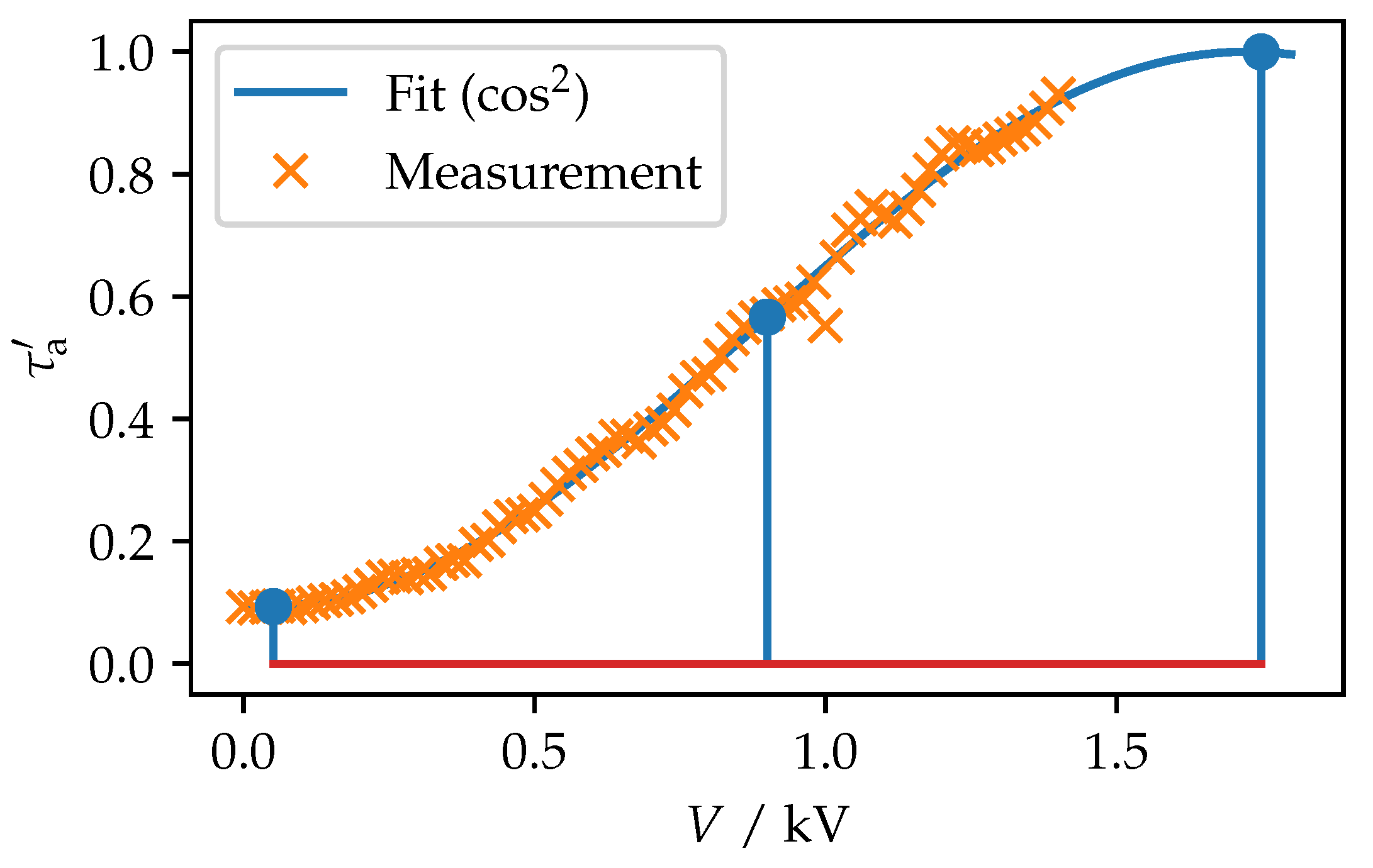
In order to validate the analytical results, they are compared with the measurements. First, we determine the half-wave voltage of the PS by measuring radiation intensity $I_{\mathrm{a}}$ in one of the interferometer arms while continuously increasing the applied DC voltage from 0 to $1.4$ $\mathrm{k}$$\mathrm{V}$, close to the upper limit of our voltage supply. The normalized measured values (orange crosses) with fitted squared cosine function $I_{\mathrm{fit}}$ (blue line) are shown in Figure 5. Scipy’s curve_fit() function was used to fit the data, which is a non-linear least squares optimization. Scipy is a Python library for scientific computing. Normalization is archived by dividing the measured transmission by the maximum transmission of the fitted function ${\tau }_{\mathrm{a}}^{\prime }=I_{\mathrm{a}}/max\left(I_{\mathrm{fit}}\right)$. At maximum destructive interference, 10% of the normalized transmission is retained, resulting in a resulting modulation depth of 90%.

The half-wave voltage $V_{\lambda /2}$ corresponds to the difference between the applied voltage at minimum transmission (left blue marker) and the applied voltage at maximum transmission (right blue marker). The so-called quadrature point (middle blue marker) is exactly in between the two points of maximum and minimum transmission. It is often used as the preferred operating point of the MZM in bias voltage control algorithms. The half-wave voltage, according to a ${cos}^2$ fit, turns out to be

$$V_{\lambda /2} = (1.697 \pm 0.083) \mathrm{k}\mathrm{V}.$$

(14)

We calculate the standard deviation error of the applied voltage $\pm \mathsf{\Delta }{V}_{\lambda /2}=\sqrt{{\sigma }_V^2}$ from the estimated variance ${\sigma }_V^2$ of the fit, provided by Scipy’s curve_fit() function.

Since the PS power supply is limited to $1.5$ $\mathrm{k}$$\mathrm{V}$, we can change the phase up to $max\left({\varphi }_{\mathrm{m}}\right)=0.88\pi$ only, calculated by Equation (6a). For a pure sinusoidal signal, $max\left({\varphi }_{\mathrm{m}}\right)=\pi$ would be necessary; this is also reflected in the further measurements.

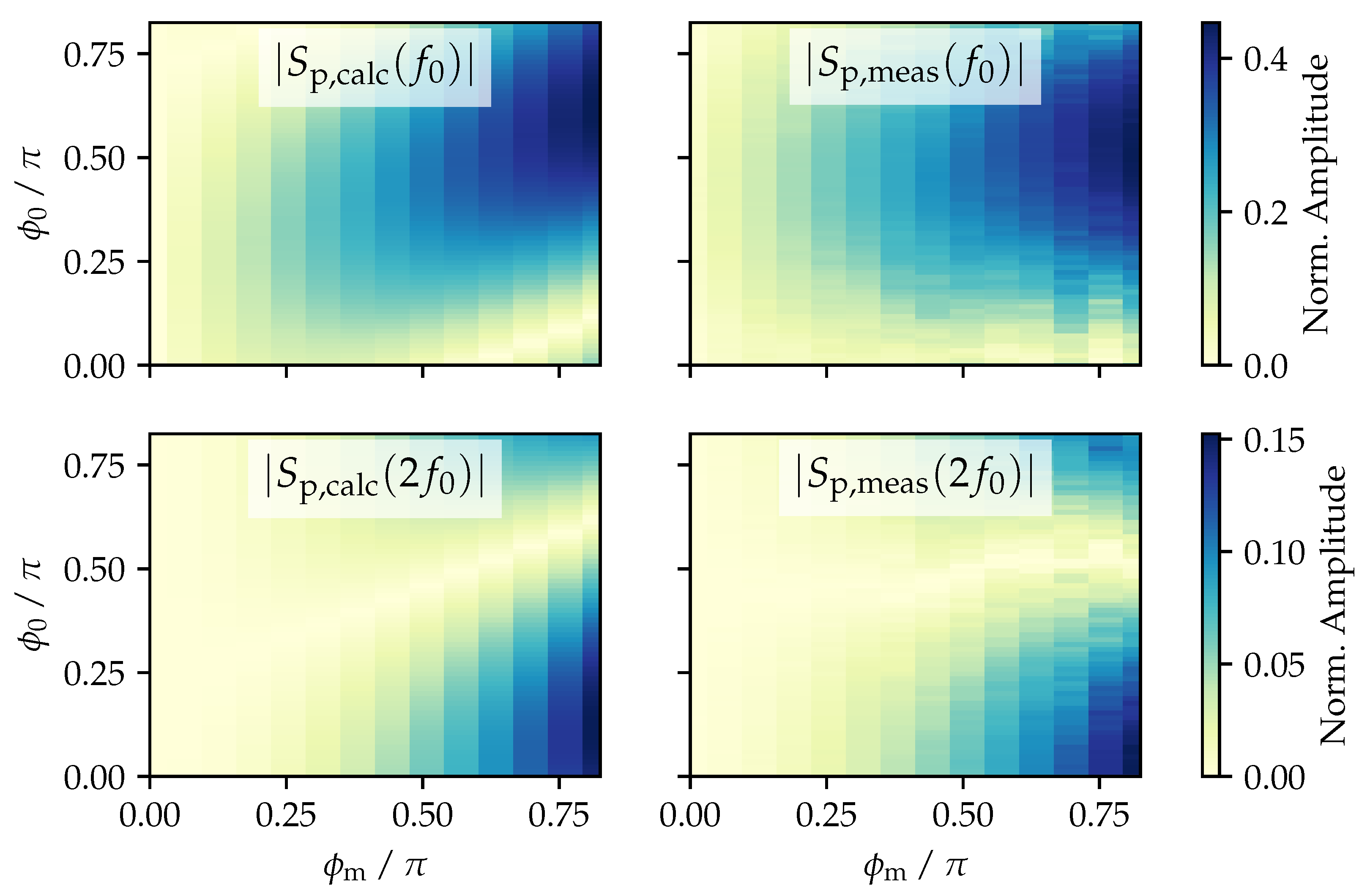
From the presented analytical description of the MZM, the frequency-dependent signal $S_{\mathrm{p},\mathrm{calc}}\left(f\right)$ can be determined for any ${\varphi }_0$, ${\varphi }_{\mathrm{m}}$, and $f_{\mathrm{m}}$. Figure 6 presents the results from the analytical model, as well as amplitudes of the measured signal $S_{\mathrm{p},\mathrm{meas}}\left(f\right)$ with the same parameters for ${\varphi }_0$, ${\varphi }_{\mathrm{m}}$, and $f_{\mathrm{m}}$. The modulation frequency of the measurement $f_{\mathrm{m}}$ is set to $2.5$ $\mathrm{k}$$\mathrm{Hz}$ and the sampling rate to 125 $\mathrm{k}$$\mathrm{Hz}$ with a duration of 2 $\mathrm{m}$$\mathrm{s}$. Matlab’s implementation of the Goertzel algorithm [13,14] was used to determine the signal amplitudes of single selectable frequencies $S_{\mathrm{p},\mathrm{meas},\mathrm{raw}}\left(f\right)$, which are then normalized by

$$S_{\mathrm{p},\mathrm{meas}}\left(f\right)=S_{\mathrm{p},\mathrm{meas},\mathrm{raw}}\left(f\right)\frac{max\left(S_{\mathrm{p},\mathrm{calc}}\left(f\right)\right)}{max\left(S_{\mathrm{p},\mathrm{meas},\mathrm{raw}}\left(f\right)\right)}.$$

(15)

The top row shows the fundamental signal $S_{\mathrm{p}}\left(f_0\right)$ and the bottom row first harmonic signal $S_{\mathrm{p}}\left(2f_0\right)$. The analytical results are on the left side, while the right side shows the measured values. In each diagram, the x-axis represents ${\varphi }_{\mathrm{m}}$, while the y-axis represents ${\varphi }_0$. The color shows the amplitude of the resulting signal $\left|S_{\mathrm{p}}\left(f\right)\right|$ for the respective constellation: dark blue represents a high and light yellow a low amplitude.

To compensate, the external factors C in (6b), the calculations are shifted along the y-axis by $C=0.12\pi$. Qualitatively, calculation and measurement match well. The difference can quantitatively be expressed by the normalized Mean Absolute Error (nMAE)

$$\mathrm{nMAE}=\frac{{\sum }_{i=1}^n|{\left(S_{\mathrm{p},\mathrm{calc}}\right)}_i-{\left(S_{\mathrm{p},\mathrm{meas}}\right)}_i|}{{\sum }_{i=1}^n{\left(S_{\mathrm{p},\mathrm{calc}}\right)}_i},$$

(16)

where ${\left(S_{\mathrm{p},\mathrm{meas}}\right)}_i$ is a single measured signal and ${\left(S_{\mathrm{p},\mathrm{calc}}\right)}_i$ is a single calculated signal.

For the fundamental we calculated a $\mathrm{nMAE}\left(S_{\mathrm{p}}\left(f_0\right)\right)=19.40\%$ and for the 1st harmonic $\mathrm{nMAE}\left(S_{\mathrm{p}}\left(2f_0\right)\right)=20.83\%$. We suspect fluctuations of ${\varphi }_0$ caused by external factors C, e.g., slight temperature changes or fluctuations in the OPO’s emission wavelength during the measurement to be the reason for the deviations of the experimental results. All the data used in our analyses are available in the Supplementary Materials, along with a detailed documented source code.

In real-world applications, the extinction ratio can be rather small; this leads to a smaller amplitude of $S_{\mathrm{p}}\left(f\mathrm{m}\right)$ and may also introduce a higher DC part of the signal $S_{\mathrm{p},\mathrm{meas}}(f=0)$. The response of the transmission to the phase difference and the phase difference to the voltage of our setup was consistent with the assumption of an ideal MZM.

6. Discussion and Conclusions

The advantages of MZMs in PAS applications are high-frequency modulation, frequency stability, and versatility for a range of applications in environmental monitoring, biomedical imaging, and materials science. We use it in combination with an OPO light source in the mid-infrared region to measure the broadband absorption features of different VOCs.

Instead of calculating the MZM signal in the time domain and then transferring it to the frequency domain, we provide a mathematical model with which the MZM signal can be determined directly in the frequency domain. Thanks to this novel method, the signal amplitudes of different frequencies can be determined efficiently and easily. The model of a MZM is valid for the case of the triangular voltage modulation of the PS. The analytical results were validated by measurements with matching parameters for ${\varphi }_0$ and ${\varphi }_{\mathrm{m}}$. We link the remaining difference between measurement and calculation to experimental uncertainties. To reduce the experimental uncertainties, the MZM’s path length difference should be reduced to minimize the influence of wavelength and temperature on the interferometer.

The new understanding of the frequency domain of the MZM is to be incorporated into a new voltage control of the PS in the future. It is also conceivable to determine the wavelength using the signal from the MZM, which would eliminate the need for an additional wavemeter and represent both a cost reduction and simplification of our experimental setup.

The presented MZM operates in the mid-infrared region, which is of interest for many spectroscopic applications, but not easily accessible. It is not often used because the wavelength dependency of the PS leads to very high half-wavelength voltages, which is also the reason why our validation is limited to the range of the phase ${\varphi }_{0,\mathrm{m}}$ from 0 to $0.82\pi$ due to the maximum possible PS voltage. The knowledge gained from this study will be used in the future to ensure a reliable pure sinusoidal modulation at voltages below the half-wave voltage.