Article

Non-Collinear Attosecond Streaking without the Time Delay Scan

1
Center for Attosecond Science and Technology, Xi’an Institute of Optics and Precision Mechanics, Chinese Academy of Sciences, Xi’an 710119, China
2
University of the Chinese Academy of Sciences, Beijing 100049, China
3
Key Laboratory of Ultrafast Photoelectric Diagnostics Technology, Xi’an Institute of Optics and Precision Mechanics, Chinese Academy of Sciences, Xi’an 710119, China
*
Authors to whom correspondence should be addressed.
Photonics 2023, 10(3), 331; https://doi.org/10.3390/photonics10030331
Submission received: 28 February 2023 / Revised: 15 March 2023 / Accepted: 17 March 2023 / Published: 20 March 2023
(This article belongs to the Special Issue Ultrafast Optics and Applications)

Abstract

:
Attosecond streaking provides an extremely high temporal resolution for characterizing light pulses and photoionization processes with attosecond (10−18 s) accuracy, which employs a laser as a streaking field to deflect electrons generated by photoionization. The current attosecond streaking requires a time delay scan between the attosecond pulses and streaking field with attosecond accuracy and a femtosecond range, which is difficult to realize real-time measurement. In this study, we theoretically propose a non-collinear attosecond streaking scheme without the time delay scan, enabling real-time and even the potential to perform single-shot attosecond pulse measurement. In the proposal, time-delay information is projected into longitudinal space, both horizontally and vertically, enabling attosecond pulse characterization with temporal-spatial coupling. From our calculation, down to 70 as pulses with pulse front and wavefront tilt are characterized with high accuracy. Our study not only provides a method toward real-time attosecond pulse measurement, but also an approach for attosecond pump-probe experiments without time delay scan.

1. Introduction

At the beginning of this century, generation of attosecond pulses was demonstrated and reported [1,2,3]. Subsequently, attosecond pulses have been employed in a variety of pioneering ultrafast research fields [4,5,6,7,8,9]. Because the attosecond pulse is currently the shortest pulse that scientists can generate [10,11], there is no method that can be employed for directly characterizing its temporal information. Thus, several schemes have been proposed and demonstrated to indirectly characterize attosecond pulses such as laser-assisted lateral x-ray photoionization [12], reconstruction of attosecond harmonic beating by interference of two-photon transitions (RABBITT) [13], and the attosecond streak camera [14], which requires a retrieval algorithm to obtain the pulse duration and chirp of attosecond pulses. Frequency-resolved optical gating for complete reconstruction of attosecond bursts (FROG-CRAB) [15,16] is one of the mostly employed techniques. This method is valid when central momentum approximation (CMA) is applicable, which requires that the bandwidth is small compared with the central wavelength of the attosecond pulses. Another method, Phase Retrieval by Omega Oscillation Filtering (PROOF) [17], was proposed to circumvent the CMA limitation in FROG-CRAB and could be used to characterize broadband attosecond pulses. However, PROOF limits one to streaking fields that are within the perturbative intensity regime and is restricted to relatively longer streaking pulse durations. Later, several other algorithms were developed to improve the retrieval of attosecond pulses, such as ePIE [18], VTGPA [19], PROBP [20,21], and iPROOF [22]. In 2019, an algorithm using the neural network method [23] was proposed, and was able to retrieve attosecond pulses instantaneously. Besides the retrieval of attosecond pulses from the photoelectron spectrogram, there is another kind of all-optical attosecond pulse characterization method [24,25,26,27], in which the attosecond pulse generation process is perturbed by an extra weak laser pulse, and the generated attosecond pulse spectrum is collected to retrieve its temporal information. All the methods mentioned above are based on time-consuming experimental setups that conduct a time delay scan between the measured attosecond pulse and an extra infrared (IR) laser pulse. This experiment runs for tens of minutes or even hours to collect one set of spectrogram data. Therefore, it is unsuitable for real-time measurement and especially difficult for the characterization of low repetition rate attosecond pulses [28]. Recently, a 10 Hz gigawatt-class attosecond pulse was generated and characterized by directly collecting time-of-flight (TOF) electron signals with an oscilloscope instead of a digital converter in the counting mode, after great effort to improve the long-term stability of the entire laser system [29]. Thus, the attosecond pulse characterization method, which enables real-time measurement is highly demanded.
In this paper, we theoretically propose a non-collinear attosecond streaking method, which projects the time-delay information into the longitudinal space along the laser propagation path, other than the conventionally used transverse space in the non-collinear setup to measure femtosecond pulses [30,31]. The space-resolved photoelectron spectrograms are then used to retrieve both the temporal and wavefront information of the measured attosecond pulses. Because no delay scan is required, our proposal enables real-time attosecond pulse measurement. With a proper photoelectron imaging and detection system, this non-collinear setup will even enable single-shot attosecond streaking if the space-charge effects can be dealt with carefully and properly. Moreover, attosecond pump-probe experiments on gaseous atoms or molecules can also be carried out employing this method, which facilitates the evaluation of the evolution of the ultrafast dynamics.

2. Scheme and Methods
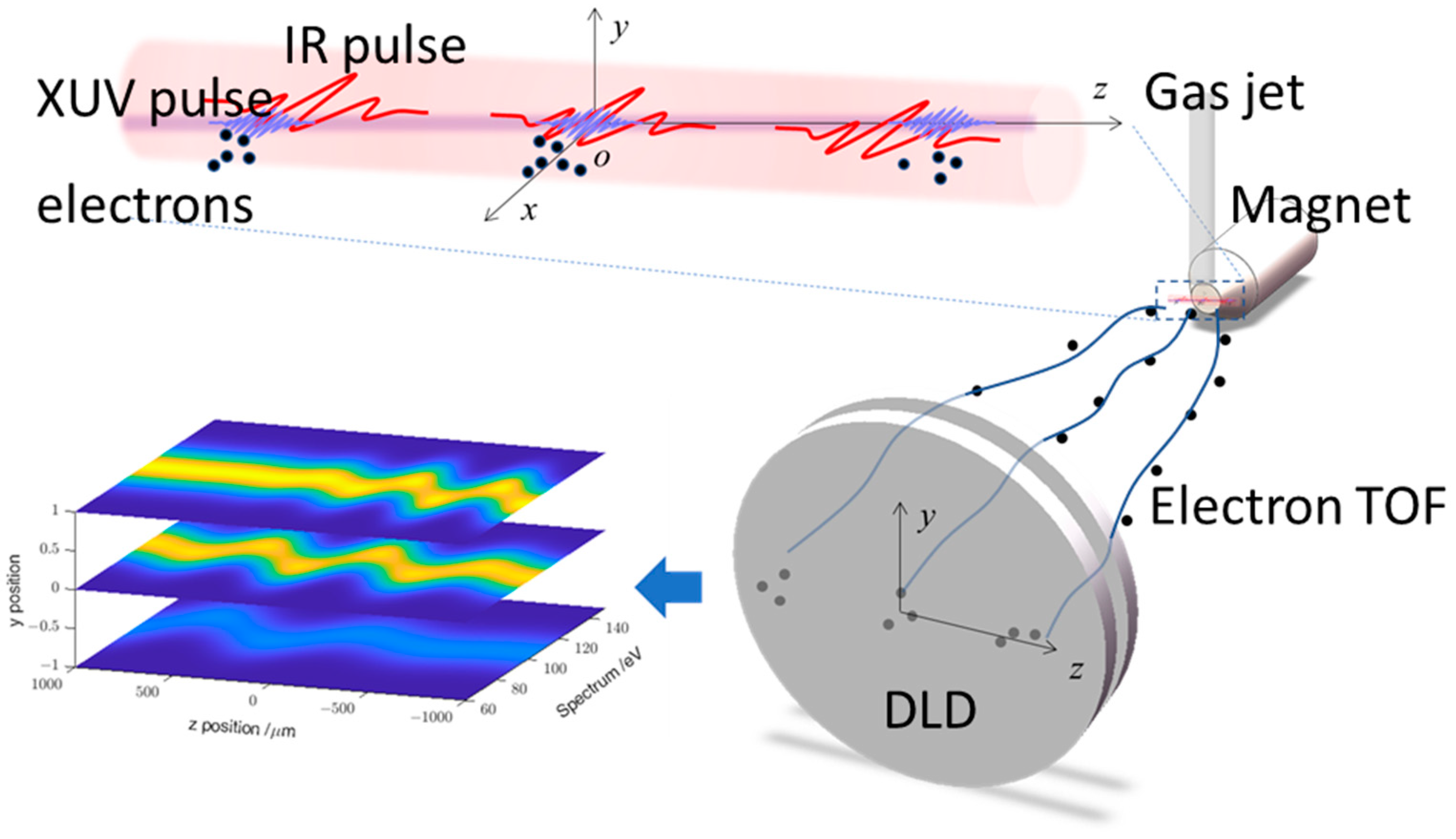
2.1. General Scheme

The attosecond streak camera measures the energy spectrum of photoelectrons from the ionization of inert gas atoms by the measured extreme ultraviolet (XUV) pulse in the presence of a collinearly propagated IR laser pulse. For a certain inert gas, e. g. argon, the photoionization cross-section is nearly constant over the bandwidth of the current attosecond XUV pulses obtained through spectral filtering, the transition dipole matrix element can be assumed to be constant and is safely ignored [32]. The obtained spectrogram S(p, τ) of the photoionized electrons can be expressed as Equation (1), under the single active electron approximation [15]
S p , τ = E X t τ exp i φ t exp i p 2 2 + I p t d t 2
φ t = t p c A I R t + A I R 2 t 2 d t
In these expressions, p is the final momentum of the electron in the continuum,   p c is the central momentum of the unstreaked photoelectrons, I p is the ionization potential of the atom, τ is the delay between the XUV and IR pulses, A I R t is the vector potential of the IR pulse and A I R t = t E I R t d t , E X t represents the complex value of the XUV field, and φ t is the quantum phase shift that the electron acquires because of its interaction with the IR laser field after the moment of ionization. Equations (1) and (2) are expressed in atomic units.
For the method proposed in this paper, time delay τ in Equation (1) can be mapped into the propagation distance z . As shown in Figure 1, the x-polarized XUV and IR pulses propagate along the z axis through a low pressure gas medium with a small angle θ between them on the y-z plane. XUV pulse at different positions thus experience different time delays from the streaking IR pulse. Spatially resolving the energy spectrum of the electrons on the y-z plane will finally yield
S p , z , y = E X t , z , y exp i φ t , z i r , y i r exp i p 2 2 + I p t d t 2
φ t , z i r , y i r = t p c A I R t , z i r , y i r + A I R 2 t , z i r , y i r 2 d t
where z i r = z cos θ y sin θ , and y i r = z sin θ + y cos θ in Equation (3). These are the general equations without considering the available spatial resolution from the photoelectron imaging system and delay-line-detector (DLD). The sliced streaking traces in the lower left of Figure 1 are from different lines of the DLD output data, e.g., S p , z , y = 1 ,   0 ,   1 .

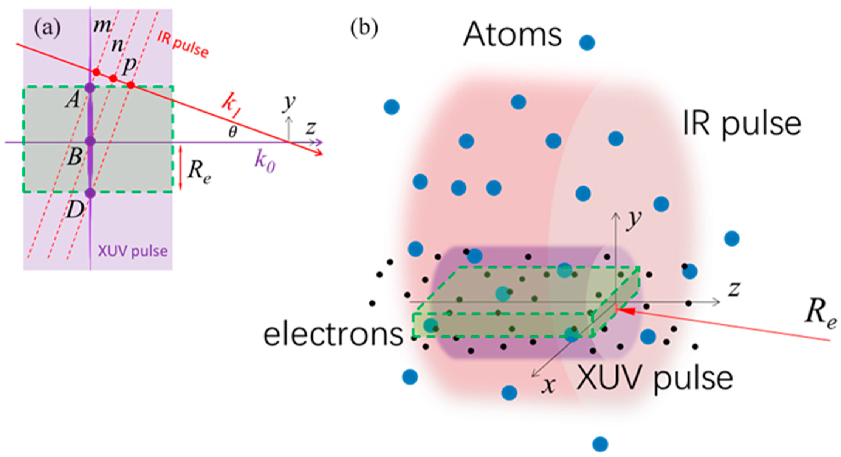
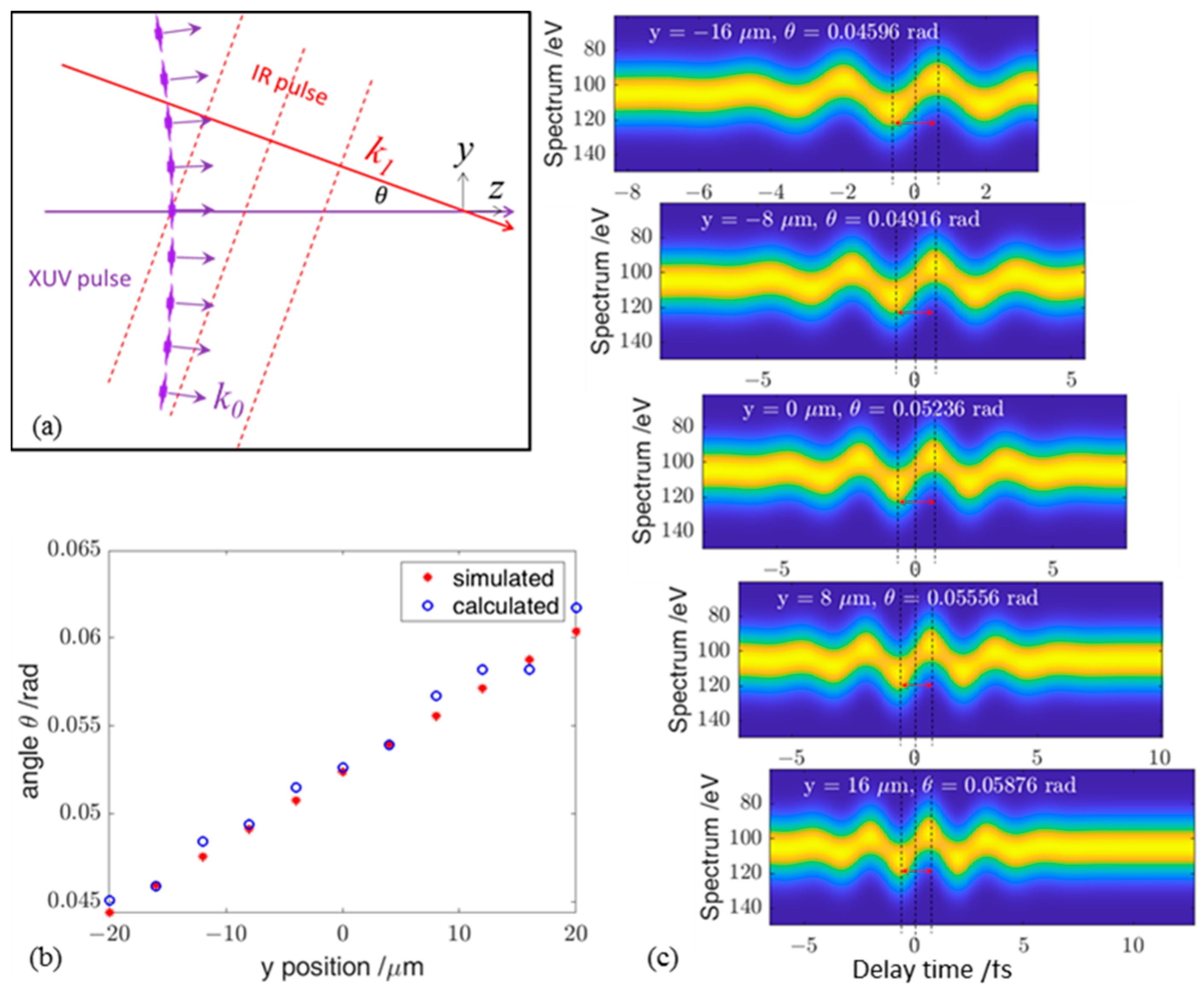
2.2. Mapping Time-Delay to Space

Mapping time-delay to a transverse plane of two non-collinearly propagated laser pulses has been applied in single shot femtosecond pulse characterizations [30,31]. In this paper, time-delay is mapped to the longitudinal plane to detect photoelectrons generated along the laser polarization direction, which comes along naturally with the problems of laser propagating through gas medium.
To retrieve the temporal information of the XUV pulses, Equation (3) indicates that the XUV pulse should be transparent while propagating through the gas medium. The transmission through 2 mm argon with a maximum pressure of 1 Pa in the 20–300 eV range is calculated [33] to be higher than 99.7%, which is good enough for the retrieval of the XUV pulses.
For the refraction of the XUV and IR lasers, according to [34,35],
n x u v = 1 1 / 2 π · N r e λ 2 f 1 n i r 2 = 1 + p p 0 · T 0 T · B 1 λ 2 λ 2 C 1 + B 2 λ 2 λ 2 C 2 p 0 , T 0
where N is the number of atoms per unit volume, re is the classic electron radius, f1 is the scattering factor of atoms which can be found in [33], and nir is the Sellmeier formula for gases. For XUV pulses centered at 85 eV and IR lasers centered at 800 nm, the refraction-induced relative delays between them are z n i r n x u v / c , which is far less than 1 as for z = 2 mm under argon gas pressure of 1 Pa. The carrier-envelope-phase (CEP) change of the few-cycle IR pulse itself has also been calculated and is less than 1 μrad, which is neglectable.
If the two pulses are both spatially and temporally overlapped at z = 0, then the relative time delay from the angle induced light path difference at position z will be
Δ t z = z z cos θ / c
which introduces a time-delay of 9.1 fs for a propagation range of 2 mm and angle of 3 degrees. Increasing the propagation range or cross angle θ will increase the effective time delays between the two pulses. By loosely focusing the IR field with a Rayleigh length z R 1 larger than 100 mm, the geometrical phase variation tan 1 ( z / z R 1 ) can be controlled to be less than 20 mrad (an extra time-delay of 8 as through a propagation range of 2 mm), which could be neglected compared with the time delay introduced by the propagation angle.

2.3. Time-Delay Resolution

Because time-delay is mapped to the propagation distance z, the spatial resolution along this direction will serve as a time-delay resolution based on Equation (5), which is similar to the time-delay of driving laser in a collinear attosecond streaking setup [36,37], or the phase variation of the laser field mentioned in [14]. A spatially resolved photoelectron spectrogram could be realized through magnetic-bottle time-of-flight (MB-TOF) technology [38,39,40], which has been mainly used as a point source electron spectrometer in the attosecond streaking community [41,42]. Photoelectrons from the initial ionization location are imaged to the front surface of the final DLD [43] or a MCP detector with a phosphor screen followed by a Timepix3 camera [44], which have both temporal and spatial resolutions, to obtain the spectrogram data of S p , z , y .
The schematic diagram of the laser-atom interaction zone is shown in Figure 2b. The IR beam size is much larger than that of the XUV beam. Photoelectrons are generated along the XUV beam path through single photon ionization in the presence of the IR laser field. A portion of the generated electrons, indicated inside the dashed rectangular green box, will be collected along the polarization direction to obtain its electron spectrogram. Photoelectrons at different positions on the longitudinal plane experience different time delays of the IR laser, which is illustrated in detail by the longitudinal cross section of the setup in Figure 2a. Limited by the spatial resolution of the photoelectron imaging and detection system, the spatially unresolvable region is shown as the dashed square green box, with half height R e . Point A, B, and D are electron sources within the unresolved region and the corresponding positions of the streaking IR fields are marked by dashed tilted red lines m, n and p. Thus, the time delay resolution is 2 R e s i n θ / c along y axis, and 2 R e 1 c o s θ / c along the z axis. The ratio s i n θ / 1 c o s θ is 38 with an angle of 3 degrees. This means that the time delay resolution will mainly depend on the spatial resolution along the y axis. Therefore, the final spectrogram at a certain position z0 will be smeared as a summation of all the electrons within this region,
S s m e a r p , z 0 = R e R e S p , z 0 , y d y
When the spatial resolution is not high enough, collecting electrons from a narrow slice along the XUV beam path can decrease this time-delay smearing effect.

2.4. XUV Pulse Retrieval

In this paper, PCGPA [15] and ePIE are employed for the pulse retrieval. Because attosecond streaking from a point source is extended to a 2D spatial region, the laser functions of time and 2D space should be considered. The femtosecond IR Gaussian pulse can be written as [45],
E I R t , z , r 1 = i i + z z R 1 exp 2 l n 2 t z / c 2 τ 1 2 + i ω 1 t k 1 z + φ 1 r 1 2 w 1 2 i i + z z R 1
with c as the speed of light, τ 1 as the pulse duration (i.e., the full width at half maximum of the intensity envelope), ω 1 as the central frequency, φ 1 as the carrier envelope phase, k 1 as the wave vector, z R 1 = π w 1 2 / λ as the Rayleigh length, and w 1 as the beam waist. To fit the retrieval algorithm, Equation (7) must be simplified to a function of only t and z, and z should function the same as t.
This could be accomplished if we focus on the temporal structure of the XUV field and assume that both the XUV and IR pulses are loosely focused. In this way, the Rayleigh length z R 1 is much larger than the propagation distance z , and laser Equation (7) can be simplified to
E I R = E I R 1 t z / c E I R 2 r 1
Similarly, the XUV pulse could be written as
E X = E X 1 t z / c E X 2 r 0
Thus, Equation (3) becomes
S p , z , y = E X 2 2 y E X 1 t z / c exp i φ t z i r c , y i r exp   i p 2 2 + I p t d t 2
E I R 2 y in the phase function φ t z i r / c , y i r can be viewed as the streaking laser intensity variation, which was studied in [37]. Equation (10) shows that this spectrogram could be used to retrieve the attosecond XUV field using the FROG-CRAB method.

3. Results

We first demonstrate in the time domain that non-collinear attosecond streaking can be used to characterize XUV pulses, along with the limitations of this setup. We also identify the maximum smearing effect that is within the tolerance to accurately retrieve the attosecond XUV pulses. We then proceed to demonstrate in the spatial domain that this setup can be used to characterize the XUV pulse front tilt and wavefront tilt.

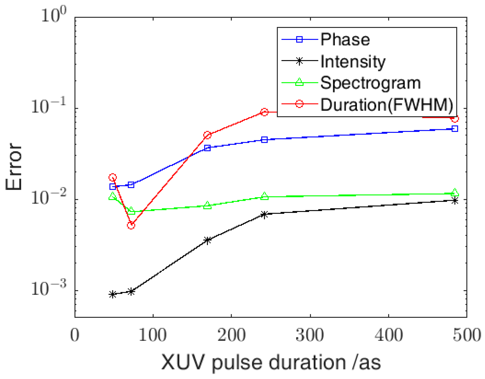
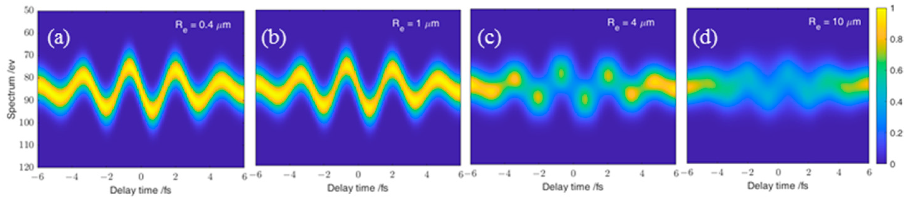
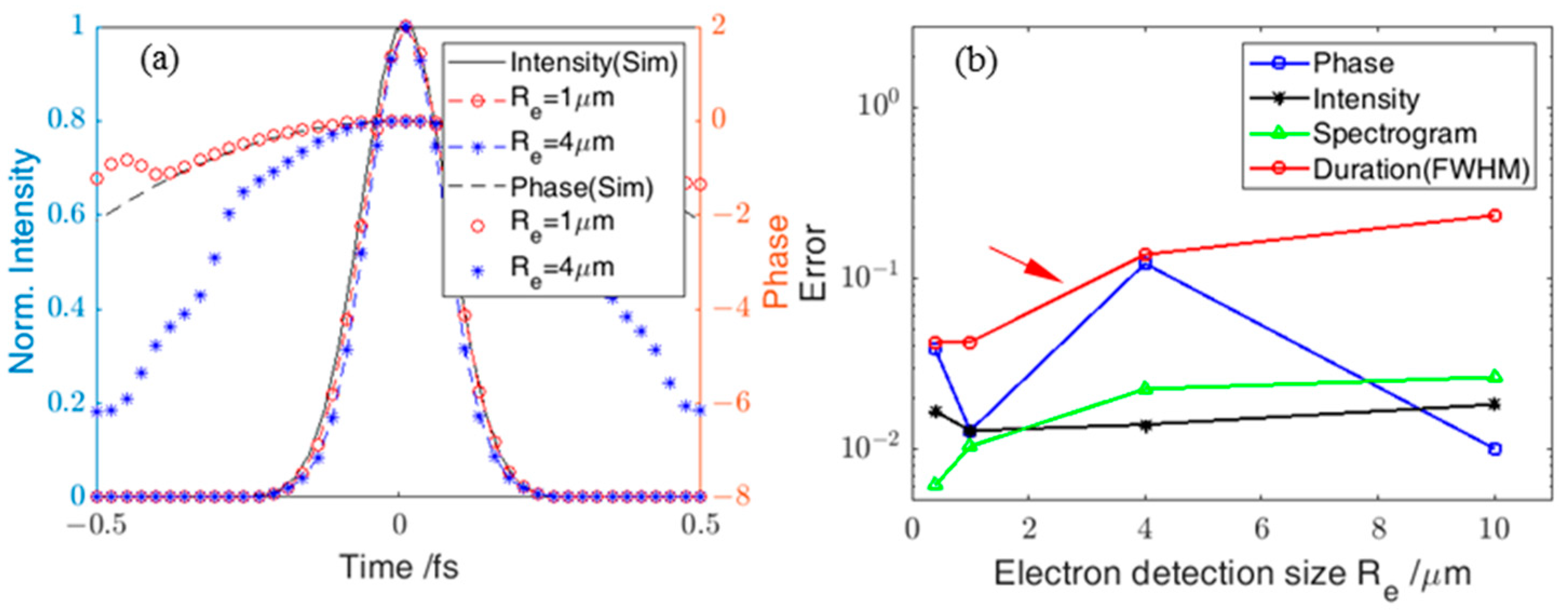
3.1. Temporal Domain Characterization

The simulated streaking IR field is centered at 800 nm, with a peak intensity of approximately 0.25 × 10¹³ W/cm2, and pulse duration of 8.9 fs with no chirp. It is relatively easy to experimentally obtain this kind of pulses because Ti: sapphire femtosecond laser is widely employed. To best fit the CMA requirement of the retrieval algorithm, the XUV field to be measured is supposed to center at 85 eV, with a pulse duration of 170 as, i.e., bandwidth of approximately 10 eV, and is linearly negative chirped in the temporal domain. The two pulses are spatially and temporally well overlapped in the center of the focus point. For simplicity, only the photoelectrons generated on the axes are considered, i.e., y = 0 in Equation (10).
When θ = 3 ° , a 2 mm detection length (i.e., propagation range of z 1 , 1   mm ) introduces a delay time of 9 fs as calculated by Equation (5). The XUV beam waist is set as 40 μm, which can be achieved experimentally. By adjusting the IR laser beam waist in Equation (7), which changes the Rayleigh length and Gouy phase of the IR beam, a set of spectrograms is obtained based on Equation (10), as shown in Figure 3. The time delay introduced from the Gouy phase as mentioned in Section 2.2 are also considered here. It can be clearly observed that the spectrograms are significantly influenced by the streaking beam size. Particularly, when it is focused to a few micrometers, the streaking laser electric field is strongly deformed along the transverse direction. Therefore, most of the spectrogram data along the time-delay axis (i.e., XUV propagation axis) are merely unstreaked XUV spectrum; only a small part around the focus point contains XUV phase information.
We use the root mean square (RMS) error to quantitatively define the convergence of the retrieval algorithm, which is defined as σ = i X r , i X s , i 2 / N , where Xr represents the retrieved data, Xs is the simulated data, and N is the data array length. The corresponding RMS errors of Figure 3 are shown in Figure 4a. The XUV pulse can be reconstructed very well with the IR beam size larger than a few tens of micrometers. However, the RMS errors start to occur when the IR beam size is below 30 μm. Two reasons may help to explain this phenomenon. First, to conduct an attosecond streaking experiment, the pulse duration of the streaking field should be no less than one cycle. This cannot be satisfied when the streaking beam is tightly focused, which can be observed from Figure 3c. Second, for this non-collinear attosecond streaking setup, the streaked XUV spectrum at different time delays are streaked by slightly different IR wave functions. This is inconsistent with the retrieval method, which aims to search for one certain XUV field and one certain streaking field. In this situation, it is confirmed that the streaking field cannot be correctly reconstructed, and neither can the XUV field. Particularly, when the IR field is tightly focused, the error will increase because the range of the streaking function that is contained within one spectrogram will increase.
For detection systems with a low spatial resolution, sparse sampling along the propagation direction could be an option. To verify whether sparsely sampled spectrogram data can be used to retrieve the XUV pulse, the ePIE method was employed. The spectrogram data were simulated for sampling at 0.49 eV per step with 512 steps covering 0 to 170 eV in the energy spectrum and 120 as per step with 128 steps starting from −7.6 to 7.6 fs in the time-delay range, respectively. The data are interpolated to 512 × 512 to satisfy the requirement of the PCGPA. For comparison, 40 samples were recorded for ePIE with no further interpolation, at 221 as per step starting from −4.3 fs to 4.3 fs for the time-delay range. The retrieved intensity and phase of the XUV pulse streaked by an IR laser with beam waist size of 100 μm are shown in Figure 4b, using both the PCGPA and ePIE method. It shows that ePIE can correctly retrieve the XUV pulse from sparsely sampled spectrogram data.
The RMS errors of the retrieval with different simulated pulse durations are shown in Figure 5. The phase and duration errors are less than 10% throughout our simulation in the range of 50 to 500 as. XUV pulse duration down to 70 as can be retrieved with good accuracy.
Photoelectrons are assumed to be generated from point sources along the XUV propagation direction in the calculations above. It is actually generated at all the places where the XUV pulse interacts with inert gas atoms, and is then collected by the imaging and detection system with a limited spatial resolution as illustrated in Figure 2. From the calculations above, the streaking IR beam waist is set at w1 = 100 μm and the XUV beam waist w0 = 40 μm. Spectrograms are calculated from Equation (6) based on the laser functions from Equations (8) and (9).
Figure 6 shows the spectrograms calculated with varied R e . The streaking trace is smeared out even when R e is as small as 10 μm. The time-delay difference along the y axis would be as high as 350 as with R e = 1   μ m , and the XUV pulse is well-reconstructed in this case as shown in Figure 7a. Figure 7b shows the RMS error of the reconstructed spectrogram and the retrieved XUV pulse phase, intensity, and pulse duration. As the red arrow points out, the error of the retrieved pulse duration is lower than 5% when R e 1   μ m , and higher than 10% when R e 4   μ m . Compared with the streaking IR laser period T0, based on our simulation, time-delay smearing of less than T0/8 can be tolerated, or more explicitly, 2 R e sin θ < λ / 8 , where λ is the central wavelength of the streaking laser. The result in our simulation matched well with the phase variation requirement ( < 2 π τ x u v / τ i r ) for the attosecond streak camera proposed by [14] and with the requirement for the driving laser jitter from [37]. Because shot noise has a slight effect on the retrieval of single attosecond pulses with the PCGPA algorithm if the photoelectron counts are not too low [37], it is not considered in our simulation.

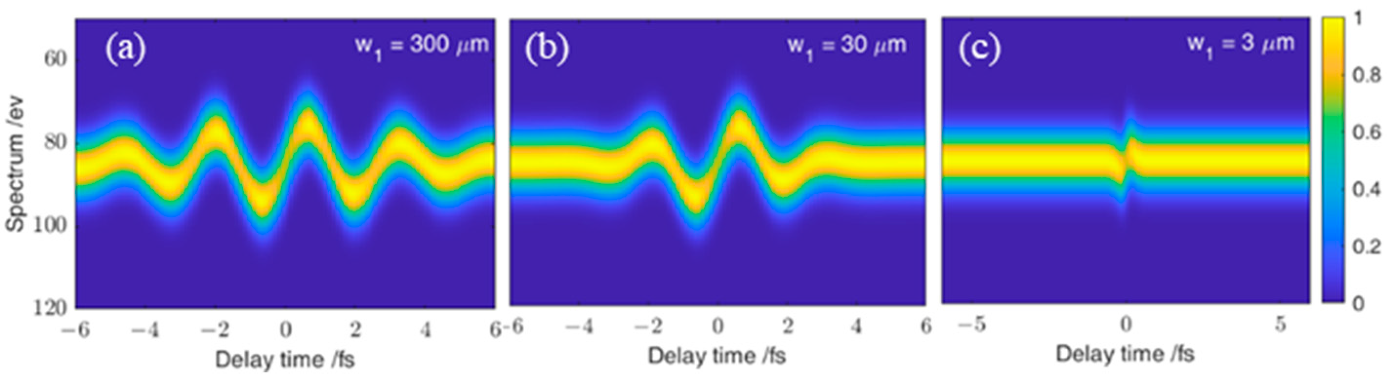
3.2. Spatial Domain Characterization

Apart from the characterization of the XUV pulse in the temporal domain, pulse front tilting and wave front aberrations of the XUV beam, can also be characterized with a spatially resolved non-collinear attosecond streaking setup, if the streaking laser beam profile is assumed to be with no aberration.
As shown in Figure 8a, the XUV pulse front is set to be tilted linearly along the y axis, which adds extra time delays between the XUV and IR pulses at different y positions, compared to the pulse on the axis. Because pulse front tilting only alters the time delay between the two pulses, the intensity and shape of the spectrograms at different y positions should remain the same, as shown in Figure 8c. The spectrogram is only shifted left or right according to the effective time delays, which comes from the shifted distance along the y axis and the XUV pulse front tilting along the propagation direction z. The former one can be calculated from y s i n θ / c , which is then used to compensate and realign the spectrogram, as indicated by the dashed black line across Figure 8c. The locations where time-delay should be the same if XUV pulse front tilting is not considered are marked by solid red circles, and the dashed red line connecting these solid red circles shows the tilted XUV pulse front, which can be detected by the spatially resolved spectrogram. Figure 8b shows the simulated and calculated pulse front tilting parameter.
We further determined whether the XUV wave front aberration can be characterized from this setup. Equation (10) indicates that any constant phase change of the XUV pulse will not change the spectrogram and thus, cannot be retrieved from the spectrogram. Therefore, wave front aberration cannot be obtained from the reconstructed XUV phase information. A schematic of the XUV wave front aberration based on the wave vector is shown in Figure 9a. The angles between the XUV and IR wave vectors are linearly changed along the y axis, with the assumption that the IR wave vector remains the same. It is indicated in Equation (5) that for a certain observation length z, the time-delay range will change nonlinearly with the angle between the wave fronts of the XUV and IR pulse. Because the streaking IR field remains the same, the spectrogram will exhibit stretched or compressed trace of the steaking IR field, which can be observed in the calculated and realigned spectrograms in Figure 9c. This nonlinear change in the time-delay range can be used to calculate the wave vectors of the XUV field, as shown in Figure 9b. In our simulation, the XUV wave vectors along the propagation direction at a certain y position are assumed to be similar. The dynamic change of the wave vector along the propagation direction can also be calculated from the changing frequency of the streaking IR field trace within a single spectrogram. Temporal information of the attosecond XUV pulses can still be retrieved accurately if the XUV wave vector does not deviate considerably. When the angle between the XUV and streaking IR laser is too large (>110 mrad) or too small (<42 mrad), the effective time-delay range of the corresponding spectrogram will also be too large or too small. For the former one, the time-delay step is so large that data in one cycle of the streaking laser is not enough for the retrieval. For the latter, the time-delay range is smaller than one cycle of the streaking laser; the spectrogram data in this situation cannot be used to correctly retrieve the XUV temporal information.

4. Discussion

The non-collinear attosecond streaking method extends the detection region from traditional point photoelectron sources to spatially resolved photoelectron sources. Thus, one needs to measure the energy spectrum S(p, z, y) from a small plane instead of only energy spectrum S(p) from a point source in the conventional attosecond streaking setup. So, in order to experimentally realize such a measurement, a proper photoelectron imaging and detection system is very important.
MB-TOF can act as electron-image magnifier, although it is more commonly used as an electron spectrometer because of its high electron collection efficiency. Its spatial resolution is around a few tens of micrometers [38] when electron energy is ~100 eV and magnetic field is near 1 Tesla. To resolve the electrons emitted from within a radius of 10 μm and minimize the smearing effect, we have simulated a MB-TOF spectrometer model with computer simulation technology (CST). Using a small pinhole array placed at ~200 μm away from the electron source, with a pinhole radius of 10 μm and a hole-to-hole distance of 50 μm, electrons from the source plane within a spot of a radius of ~10 μm can be imaged onto the detector plane placed at 330 mm away and distinguished clearly from the adjacent spot images. Because the field of view is around 1~2 mm, the trajectories of electrons emitted from the separated spots on the source plane could be very different, leading to an obvious time-of-flight difference, which can be precalculated and compensated later.
Because there is no requirement for a time delay scan, the entire detection process can be finished very fast or even in real-time if the signal is strong enough. For this reason, single shot attosecond streaking may also be possible through this non-collinear setup, if two more issues can be overcame. As far as we know, at most three electrons simultaneously hit the detector at three different locations can be recorded through DLD. Intensity information cannot be obtained during one single shot. Timepix3 camera is better for real-time application, because it can simultaneously output discrete intensity information. But due to its limited space and time resolution and the long pixel hit dead time, it will not be applicable in the single shot situation. So, one should switch to other analog methods in order to measure both the spectrum and its intensity at the same time. Space-charge effect is another universal problem one should concern when dealing with single shot photoelectron detection. There should be an upper limit of the electron density both in time and space, within which space-charge effect is not so prominent to obviously distort the spatial or energy resolution. Recent progress [28,29] show that MB-TOF can be used under high energy XUV pulses. By extending the detection source from a point to a limited 2D space, more signal counts could be collected within this space-charge limit.

5. Conclusions

To conclude, we theoretically proposed a non-collinear attosecond streaking scheme. It has the advantage of recording space resolved two-dimensional photoelectron spectrograms without the need of the time-delay scan, and can be used to characterize attosecond XUV pulses with temporal-spatial coupling. The simulation results showed that attosecond pulses with pulse duration down to 70 as can be retrieved well with the loosely focused streaking laser pulses. Pulse front tilting and wave front aberrations of the XUV pulse can also be characterized if the IR streaking field has a uniform temporal-spatial profile.

Author Contributions

Conceptualization, P.X. and Y.B.; methodology, P.X., H.C. and Y.F.; validation, Y.F., Y.W. and W.Z.; formal analysis, L.-W.P.; investigation, P.X., X.W. and H.Y.; resources, Y.F. and Y.B.; data curation, P.X. and X.W.; writing—original draft preparation, P.X.; writing—review and editing, H.C., Y.F. and L.-W.P.; supervision, Y.F.; project administration, Y.F.; funding acquisition, W.Z. All authors have read and agreed to the published version of the manuscript.

Funding

This research was funded by the National Natural Science Foundation of China (NSFC) (Nos.12104501, 62175256, 92050107, 61690222); International Key Research Program of the Ministry of Science and Technology of China (2022YFE0111500); Natural Science Basic Research Program of Shaanxi (No. 2019JCW-03); Science and Technology Program of Xi’an (No. 202005YK01); Major Science and Technology Infrastructure Pre-research Program of the CAS (No. J20-021-III); Key Deployment Research Program of XIOPM (No. S19-020-III); Innovation team in Shaanxi Province (No. J21-029-III).

Institutional Review Board Statement

Not applicable.

Informed Consent Statement

Not applicable.

Data Availability Statement

Not applicable.

Conflicts of Interest

The authors declare no conflict of interest.

References

  1. Paul, P.M.; Toma, E.S.; Breger, P.; Mullot, G.; Augé, F.; Balcou, P.; Muller, H.G.; Agostini, P. Observation of a Train of Attosecond Pulses from High Harmonic Generation. Science 2001, 292, 1689. [Google Scholar] [CrossRef] [PubMed]
  2. Hentschel, M.; Kienberger, R.; Spielmann, C.; Reider, G.A.; Milosevic, N.; Brabec, T.; Corkum, P.; Heinzmann, U.; Drescher, M.; Krausz, F. Attosecond metrology. Nature 2001, 414, 509–513. [Google Scholar] [CrossRef] [PubMed]
  3. Kienberger, R.; Goulielmakis, E.; Uiberacker, M.; Baltuska, A.; Yakovlev, V.; Bammer, F.; Scrinzi, A.; Westerwalbesloh, T.; Kleineberg, U.; Heinzmann, U.; et al. Atomic transient recorder. Nature 2004, 427, 817–821. [Google Scholar] [CrossRef] [PubMed]
  4. Drescher, M.; Hentschel, M.; Kienberger, R.; Uiberacker, M.; Yakovlev, V.; Scrinzi, A.; Westerwalbesloh, T.; Kleineberg, U.; Heinzmann, U.; Krausz, F. Time-resolved atomic inner-shell spectroscopy. Nature 2002, 419, 803–807. [Google Scholar] [CrossRef]
  5. Cavalieri, A.L.; Muller, N.; Uphues, T.; Yakovlev, V.S.; Baltuska, A.; Horvath, B.; Schmidt, B.; Blumel, L.; Holzwarth, R.; Hendel, S.; et al. Attosecond spectroscopy in condensed matter. Nature 2007, 449, 1029–1032. [Google Scholar] [CrossRef]
  6. Krausz, F.; Stockman, M.I. Attosecond metrology: From electron capture to future signal processing. Nat. Photonics 2014, 8, 205–213. [Google Scholar] [CrossRef]
  7. Schlaepfer, F.; Lucchini, M.; Sato, S.A.; Volkov, M.; Kasmi, L.; Hartmann, N.; Rubio, A.; Gallmann, L.; Keller, U. Attosecond optical-field-enhanced carrier injection into the GaAs conduction band. Nat. Phys. 2018, 14, 560–564. [Google Scholar] [CrossRef] [Green Version]
  8. Fu, Y.; Nishimura, K.; Shao, R.; Suda, A.; Midorikawa, K.; Lan, P.; Takahashi, E.J. High efficiency ultrafast water-window harmonic generation for single-shot soft X-ray spectroscopy. Commun. Phys. 2020, 3, 92. [Google Scholar] [CrossRef]
  9. Liang, J.; Zhou, Y.; Liao, Y.; Jiang, W.-C.; Li, M.; Lu, P. Direct Visualization of Deforming Atomic Wavefunction in Ultraintense High-Frequency Laser Pulses. Ultra. Sci. 2022, 2022, 9842716. [Google Scholar] [CrossRef]
  10. Li, J.; Ren, X.; Yin, Y.; Zhao, K.; Chew, A.; Cheng, Y.; Cunningham, E.; Wang, Y.; Hu, S.; Wu, Y.; et al. 53-Attosecond X-ray pulses reach the carbon K-edge. Nat. Commun. 2017, 8, 186. [Google Scholar] [CrossRef] [Green Version]
  11. Gaumnitz, T.; Jain, A.; Pertot, Y.; Huppert, M.; Jordan, I.; Ardana-lamas, F.; Worner, H.J. Streaking of 43-attosecond soft-X-ray pulses generated by a passively CEP-stable mid-infrared driver. Opt. Express 2017, 25, 27506. [Google Scholar] [CrossRef] [PubMed]
  12. Drescher, M.; Hentschel, M.; Kienberger, R.; Tempea, G.; Spielmann, C.; Reider, G.A.; Corkum, P.B.; Krausz, F. X-ray Pulses Approaching the Attosecond Frontier. Science 2001, 291, 1923. [Google Scholar] [CrossRef] [PubMed]
  13. Muller, H.G. Reconstruction of attosecond harmonic beating by interference of two-photon transitions. Appl. Phys. B 2002, 74, S17–S21. [Google Scholar] [CrossRef]
  14. Itatani, J.; Quéré, F.; Yudin, G.L.; Ivanov, M.Y.; Krausz, F.; Corkum, P.B. Attosecond Streak Camera. Phys. Rev. Lett. 2002, 88, 173903. [Google Scholar] [CrossRef] [PubMed] [Green Version]
  15. Mairesse, Y.; Quéré, F. Frequency-resolved optical gating for complete reconstruction of attosecond bursts. Phys. Rev. A 2005, 71, 011401. [Google Scholar] [CrossRef]
  16. Gagnon, J.; Goulielmakis, E.; Yakovlev, V.S. The accurate FROG characterization of attosecond pulses from streaking measurements. Appl. Phys. B 2008, 92, 25–32. [Google Scholar] [CrossRef] [Green Version]
  17. Chini, M.; Gilbertson, S.; Khan, S.D.; Chang, Z. Characterizing ultrabroadband attosecond lasers. Opt. Express 2010, 18, 13006. [Google Scholar] [CrossRef] [Green Version]
  18. Lucchini, M.; Brugmann, M.H.; Ludwig, A.; Gallmann, L.; Keller, U.; Feurer, T. Ptychographic reconstruction of attosecond pulses. Opt. Express 2015, 23, 29502. [Google Scholar] [CrossRef] [Green Version]
  19. Keathley, P.D.; Bhardwaj, S.; Moses, J.; Laurent, G.; Kärtner, F.X. Volkov transform generalized projection algorithm for attosecond pulse characterization. New J. Phys. 2016, 18, 073009. [Google Scholar] [CrossRef]
  20. Zhao, X.; Wei, H.; Wu, Y.; Lin, C.D. Phase-retrieval algorithm for the characterization of broadband single attosecond pulses. Phys. Rev. A 2017, 95, 043407. [Google Scholar] [CrossRef] [Green Version]
  21. Zhao, X.; Wang, S.-J.; Yu, W.-W.; Wei, H.; Wei, C.; Wang, B.; Chen, J.; Lin, C.D. Metrology of Time-Domain Soft X-ray Attosecond Pulses and Reevaluation of Pulse Durations of Three Recent Experiments. Phys. Rev. Appl. 2020, 13, 034043. [Google Scholar] [CrossRef] [Green Version]
  22. Laurent, G.; Cao, W.; Ben-Itzhak, I.; Cocke, C.L. Attosecond pulse characterization. Opt. Express 2013, 21, 16914. [Google Scholar] [CrossRef] [Green Version]
  23. White, J.; Chang, Z. Attosecond streaking phase retrieval with neural network. Opt. Express 2019, 27, 4799–4807. [Google Scholar] [CrossRef]
  24. Dudovich, N.; Smirnova, O.; Levesque, J.; Mairesse, Y.; Ivanov, M.Y.; Villeneuve, D.M.; Corkum, P.B. Measuring and controlling the birth of attosecond XUV pulses. Nat. Phys. 2006, 2, 781–786. [Google Scholar] [CrossRef]
  25. Kim, K.T.; Zhang, C.; Shiner, A.D.; Kirkwood, S.E.; Frumker, E.; Gariepy, G.; Naumov, A.; Villeneuve, D.M.; Corkum, P.B. Manipulation of quantum paths for space-time characterization of attosecond pulses. Nat. Phys. 2013, 9, 159–163. [Google Scholar] [CrossRef] [Green Version]
  26. He, L.; Hu, J.; Sun, S.; He, Y.; Deng, Y.; Lan, P.; Lu, P. All-optical spatio-temporal metrology for isolated attosecond pulses. J. Phys. B At. Mol. Opt. Phys. 2022, 55, 205601. [Google Scholar] [CrossRef]
  27. Yang, Z.; Cao, W.; Chen, X.; Zhang, J.; Mo, Y.; Xu, H.; Mi, K.; Zhang, Q.; Lan, P.; Lu, P. All-optical frequency-resolved optical gating for isolated attosecond pulse reconstruction. Opt. Lett. 2020, 45, 567–570. [Google Scholar] [CrossRef] [Green Version]
  28. Xue, B.; Tamaru, Y.; Fu, Y.; Yuan, H.; Lan, P.; Mucke, O.D.; Suda, A.; Midorikawa, K.; Takahashi, E.J. A Custom-Tailored Multi-TW Optical Electric Field for Gigawatt Soft-X-ray Isolated Attosecond Pulses. Ultra. Sci. 2021, 2021, 9828026. [Google Scholar] [CrossRef]
  29. Xue, B.; Midorikawa, K.; Takahashi, E.J. Gigawatt-class, tabletop, isolated-attosecond-pulse light source. Optica 2022, 9, 360. [Google Scholar] [CrossRef]
  30. Kane, D.J.; Trebino, R. Single-Shot Measurement of the Intensity and Phase of an Arbitrary Ultrashort Pulse By Using Frequency-Resolved Optical Gating. Opt. Lett. 1993, 18, 823–825. [Google Scholar] [CrossRef]
  31. Liu, Y.; Beetar, J.E.; Nesper, J.; Gholam-Mirzaei, S.; Chini, M. Single-shot measurement of few-cycle optical waveforms on a chip. Nat. Photonics 2022, 16, 109–112. [Google Scholar] [CrossRef]
  32. Gagnon, J. Attosecond Electron Spectroscopy Theory and its Application. Ph.D. Thesis, LMU Munchen, Munchen, Germany, 2010. [Google Scholar]
  33. The Center for X-ray Optics of Lawrence Berkeley National Laboratory. Available online: https://henke.lbl.gov/optical_constants/ (accessed on 9 December 2022).
  34. Chang, Z. Fundamentals of Attosecond Optics; CRC: Boca Raton, FL, USA, 2011; pp. 17–18. [Google Scholar]
  35. Börzsönyi, A.; Heiner, Z.; Kalashnikov, M.P.; Kovács, A.P.; Osvay, K. Dispersion measurement of inert gases and gas mixtures at 800 nm. Appl. Opt. 2008, 47, 4856–4863. [Google Scholar] [CrossRef] [PubMed]
  36. Zhong, S.; He, X.; Ye, P.; Zhan, M.; Teng, H.; Wei, Z. Effects of driving laser jitter on the attosecond streaking measurement. Opt. Express 2013, 21, 17498. [Google Scholar] [CrossRef] [PubMed]
  37. Wang, H.; Chini, M.; Khan, S.D.; Chen, S.; Gilbertson, S.; Feng, X.; Mashiko, H.; Chang, Z. Practical issues of retrieving isolated attosecond pulses. J. Phys. B At. Mol. Opt. Phys. 2009, 42, 134007. [Google Scholar] [CrossRef]
  38. Kruit, P.; Read, F.H. Magnetic field paralleliser for 2π electron-spectrometer and electron-image magnifier. J. Phys. E Sci. Instrum. 1983, 16, 313. [Google Scholar] [CrossRef]
  39. Dubbers, D. Magnetic guidance of charged particles. Phys. Lett. B 2015, 748, 306–310. [Google Scholar] [CrossRef] [Green Version]
  40. Sjue, S.K.L.; Broussard, L.J.; Makela, M.; McGaughey, P.L.; Young, A.R.; Zeck, B.A. Radial distribution of charged particles in a magnetic field. Rev. Sci. Instrum. 2015, 86, 023102. [Google Scholar] [CrossRef] [Green Version]
  41. Zhang, Q.; Zhao, K.; Chang, Z. High resolution electron spectrometers for characterizing the contrast of isolated 25 as pulses. J. Elect. Spectr. Rel. Phen. 2014, 195, 48–54. [Google Scholar] [CrossRef]
  42. Kurahashi, N.; Thurmer, S.; Liu, S.Y.; Yamamoto, Y.-I.; Karashima, S.; Bhattacharya, A.; Ogi, Y.; Horio, T.; Suzuki, T. Design and characterization of a magnetic bottle electron spectrometer for time-resolved extreme UV and X-ray photoemission spectroscopy of liquid microjets. Struct. Dyn. 2021, 8, 034303. [Google Scholar] [CrossRef]
  43. Hirvonen, L.M.; Becker, W.; Milnes, J.; Conneely, T.; Smietana, S.; Marois, A.L.; Jagutzki, O.; Suhling, K. Picosecond wide-field time-correlated single photon counting fluorescence microscopy with a delay line anode detector. Appl. Phys. Lett. 2016, 109, 071101. [Google Scholar] [CrossRef] [Green Version]
  44. Bromberger, H.; Passow, C.; Pennicard, D.; Boll, R.; Correa, J.; He, L.; Johny, M.; Papadopoulou, C.; Tul-Noor, A.; Wiese, J.; et al. Shot-by-shot 250 kHz 3D ion and MHz photoelectron imaging using Timepix3. J. Phys. B At. Mol. Opt. Phys. 2022, 55, 144001. [Google Scholar] [CrossRef]
  45. Pi, L.-W.; Hu, S.X.; Starace, A.F. Favorable target positions for intense laser acceleration of electrons in hydrogen-like, highly-charged ions. Phys. Plasmas 2015, 22, 093111. [Google Scholar] [CrossRef] [Green Version]
Figure 1. Illustration of the non-collinear attosecond streaking setup. x-polarized XUV and IR pulses propagate at a small angle and interacts with inert gas atoms around the focus. Photoelectrons generated within the detection region of the magnet-based TOF spectrometer are guided through the magnetic field and finally hit the DLD. The position and arrival time of the electron are recorded and transformed to the 3D electron spectrogram.
Photonics 10 00331 g001
Figure 2. Illustration of light-atom interaction region. (a) Enlarged longitudinal cross section of the XUV and IR beam. k0 and k1 are the wave vectors of XUV and IR pulses respectively and crossed at their focus points. Red dashed lines m, n, and p indicate three different IR pulse positions corresponding to photoelectrons generated at three different points A, B, and D of the XUV beam along the vertical direction, respectively. Photoelectrons generated inside the dashed square green box with half height Re are supposed to be spatially unresolved by the imaging system and DLD. (b) Inert gas atoms (large blue dot) are full around the IR laser path (large pink cylinder), whereas the photoelectrons (small black dot) are generated within the much smaller XUV beam path (small purple cylinder), which crosses through the IR beam path near the focus.
Photonics 10 00331 g002
Figure 3. Spectrograms for different beam waists of the streaking IR laser. (a) w1 = 300 μm, (b) w1 = 30 μm, (c) w1 = 3 μm.
Photonics 10 00331 g003
Figure 4. (a) RMS error between simulated and retrieved spectrogram (green triangle line), and XUV pulse phase (blue square line), intensity (black star line), and duration (red circle line). (b) Simulated intensity (black solid line) and phase (black dashed line) of XUV pulses. Retrieved intensity (red circle, blue star) and phase (red dashed-circle line, blue dashed-star line) from spectrograms with streaking IR laser beam waist of 100 μm with ePIE and PCGPA algorithm, respectively.
Photonics 10 00331 g004
Figure 5. RMS errors of the retrieved phase, intensity, spectrogram, and pulse duration from different attosecond XUV pulse durations with the same chirp and central wavelength.
Photonics 10 00331 g005
Figure 6. Spectrograms for photoelectron imaging and detection systems with different spatial resolutions. (a) Re = 0.4 μm, (b) Re = 1 μm, (c) Re = 4 μm, (d) Re = 10 μm.
Photonics 10 00331 g006
Figure 7. (a) Simulated XUV intensity (black solid line) and phase (black dashed line), retrieved intensity (red dashed-circle line, blue dashed-star line) and phase (red circle, blue star) of XUV pulses with R e = 1   μ m and R e = 4   μ m . (b) RMS error of the reconstructed spectrogram and retrieved XUV pulse phase, intensity, and duration.
Photonics 10 00331 g007
Figure 8. (a) Schematic of the XUV pulse front tilting on the longitudinal plane. (b) Simulated and calculated pulse front tilting parameter. (c) Calculated and realigned spectrograms from different y positions, ranging from −8 μm to 8 μm.
Photonics 10 00331 g008
Figure 9. (a) Schematic of the XUV wave front aberration. XUV wave front at different y positions with different wave vectors. (b) Simulated and calculated angles between wave vectors of the XUV and streaking IR laser at different y positions. (c) Simulated and realigned spectrograms from different y positions, ranging from −16 μm to 16 μm.
Photonics 10 00331 g009
Disclaimer/Publisher’s Note: The statements, opinions and data contained in all publications are solely those of the individual author(s) and contributor(s) and not of MDPI and/or the editor(s). MDPI and/or the editor(s) disclaim responsibility for any injury to people or property resulting from any ideas, methods, instructions or products referred to in the content.

