Ensquared Energy and Optical Centroid Efficiency in Optical Sensors: Part 1, Theory


Abstract
:
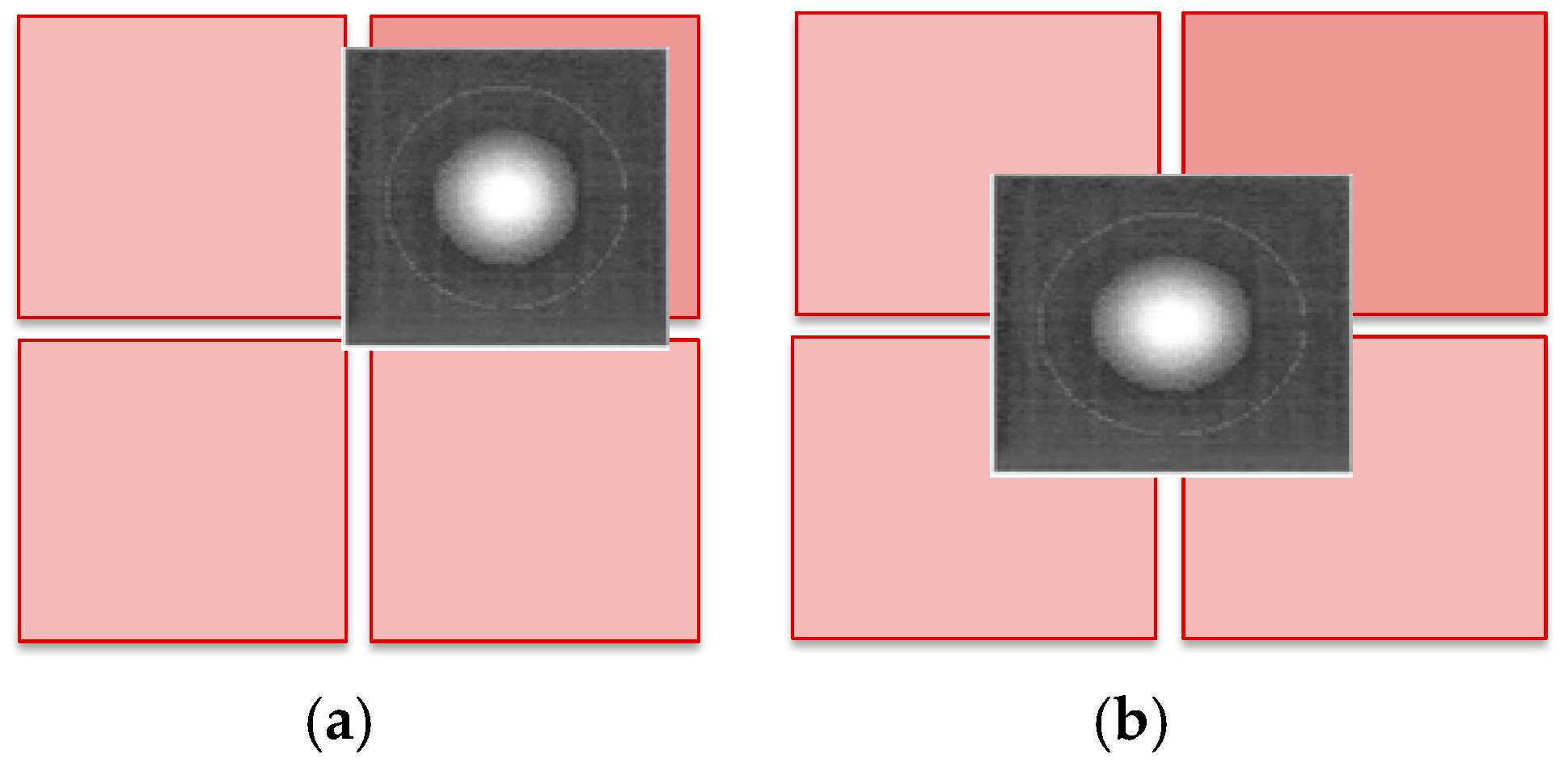
1. Discrete Pixels
2. Energy Interception by Discrete Pixels
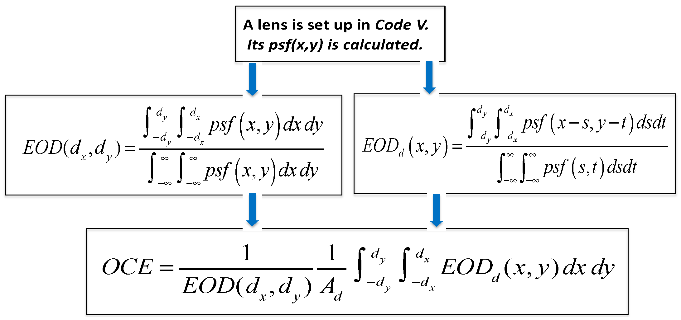
2.1. Energy on Detector (EOD)
2.2. Optical Centroiding Efficiency (OCE)
3. Imaging Theory When Optical and Detector Axes Are Arbitrarily Displaced
3.1. Image Radiometry of a Point Source
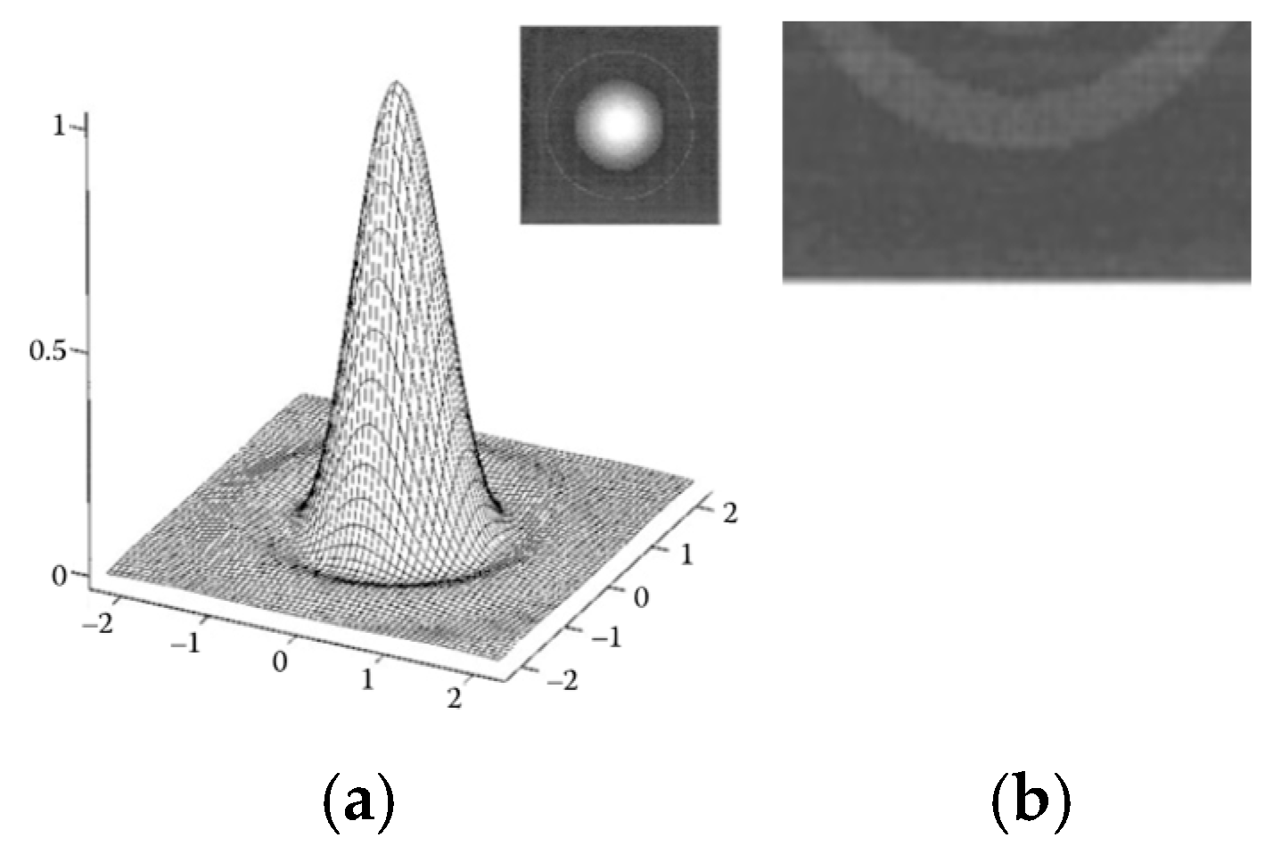
3.2. Instrument Characteristic Function
4. Modeling and Methods
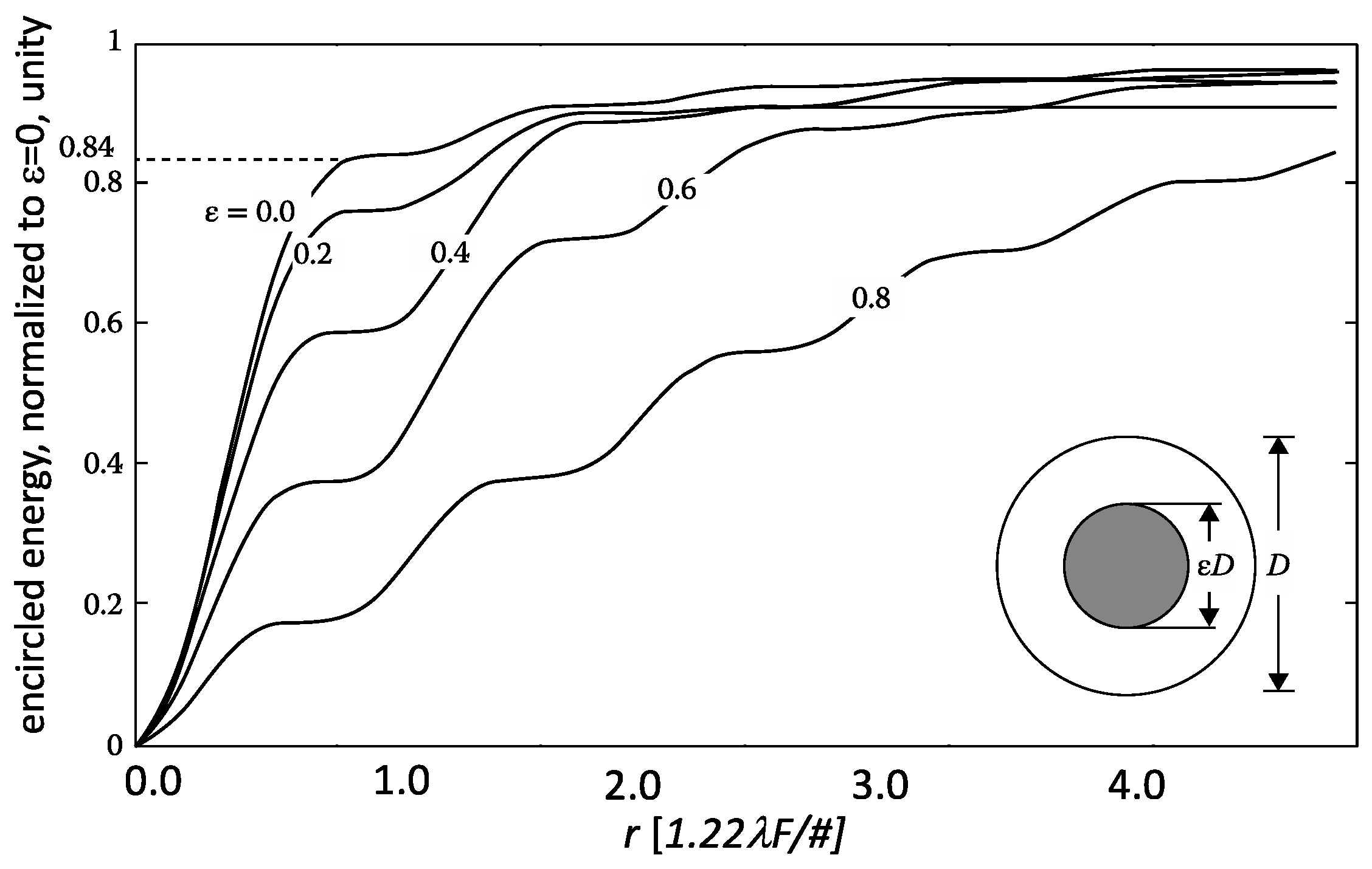
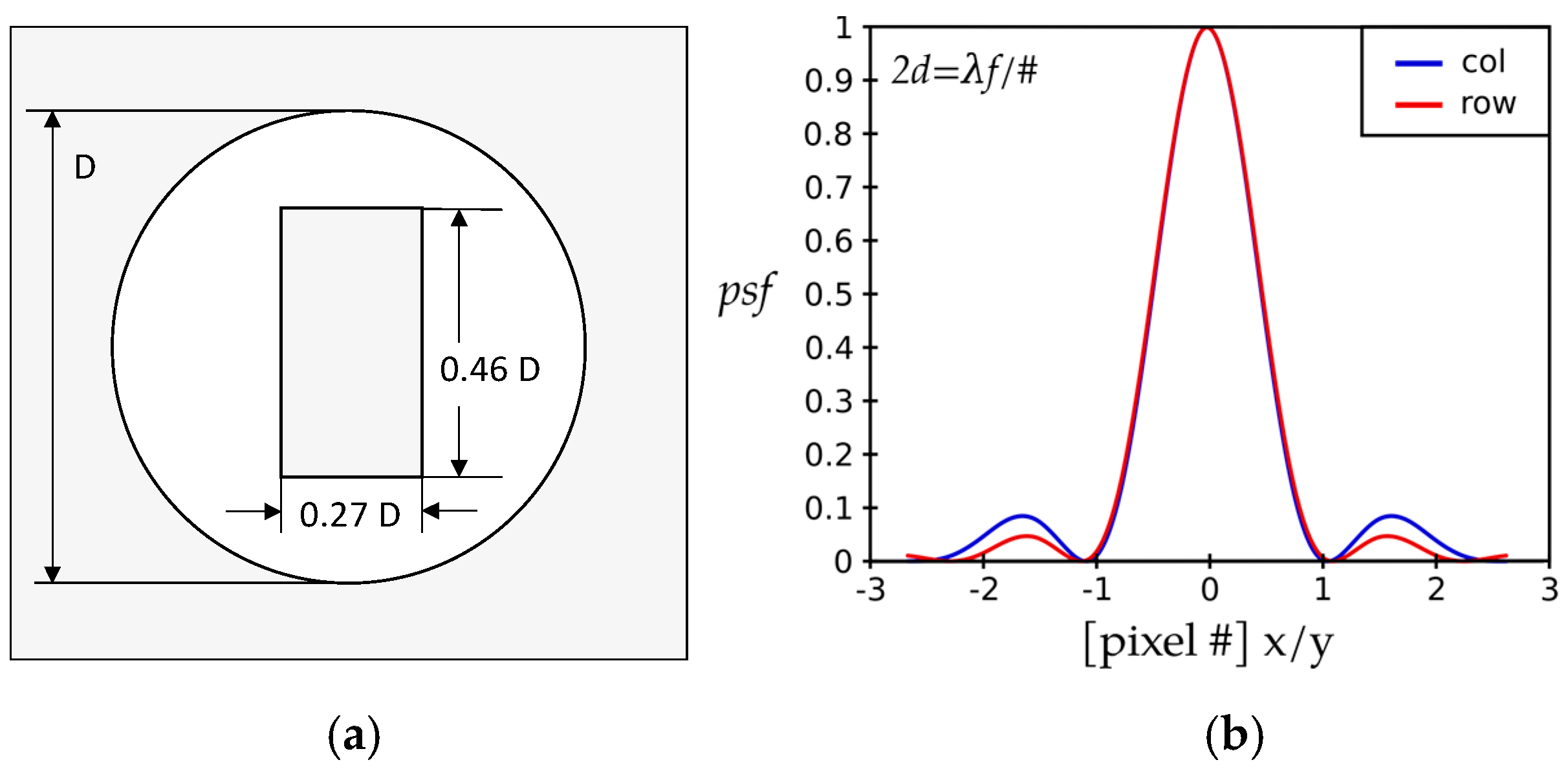
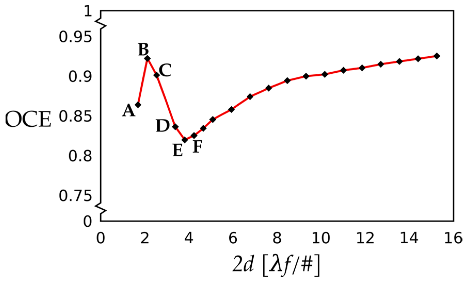
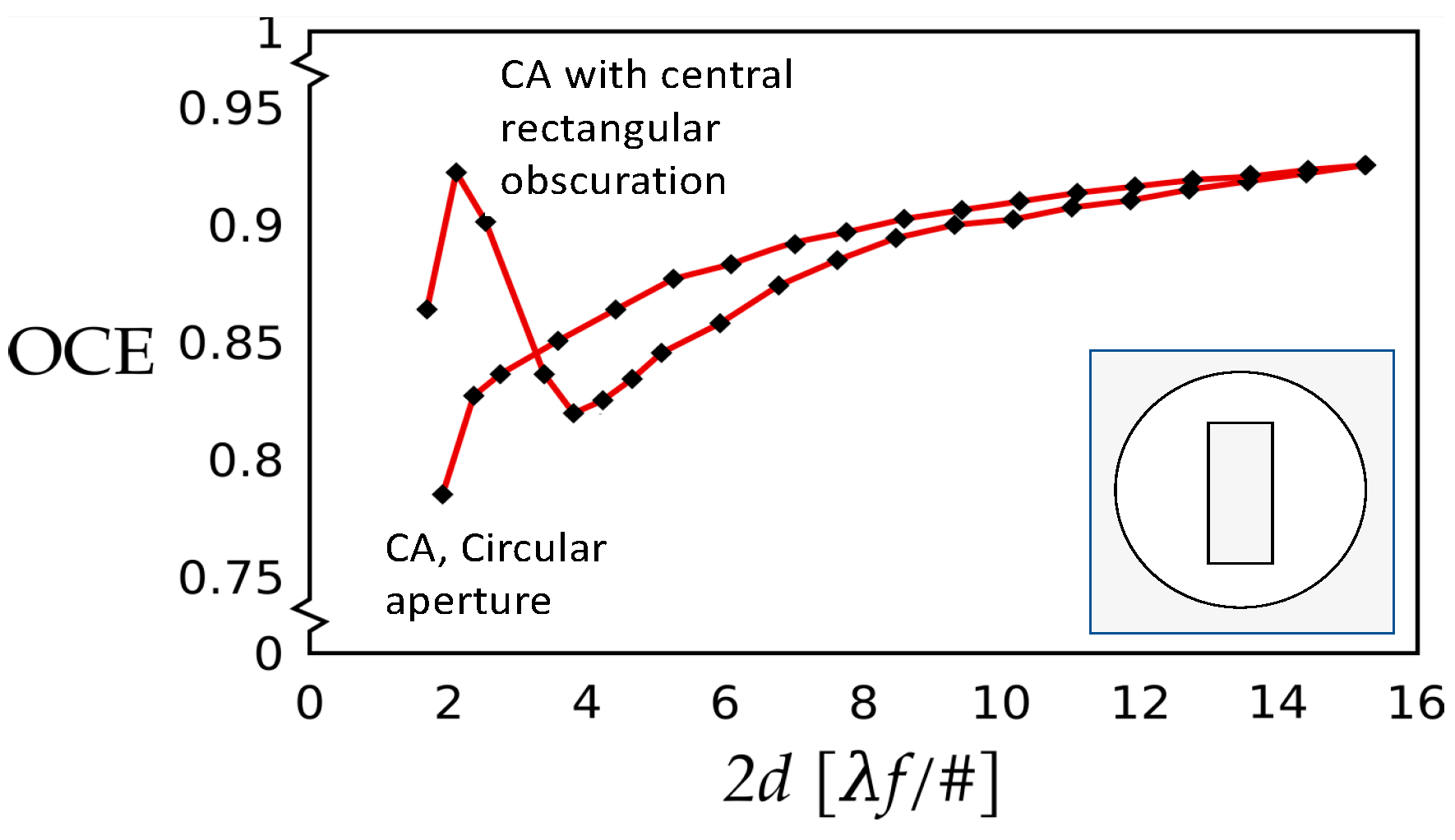
5. Effects of Pixel Size and Central Obscuration
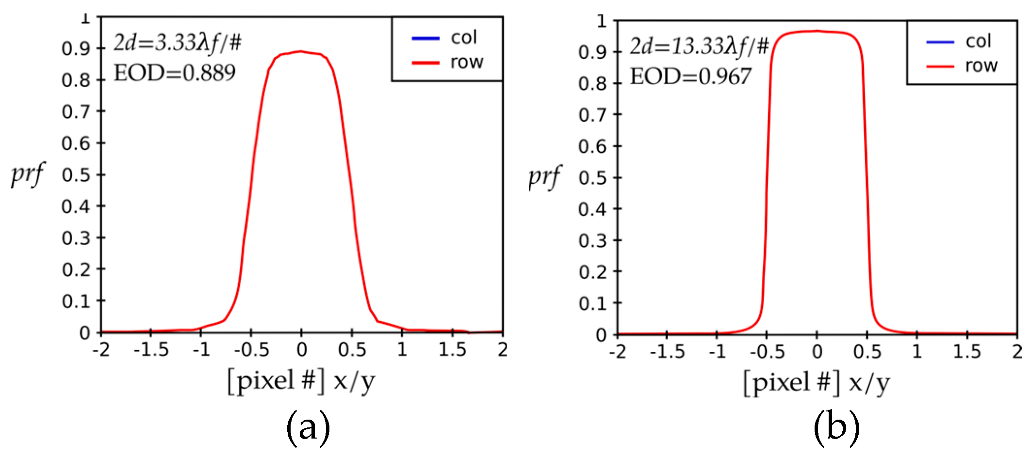
5.1. Aperture Configuration: No Central Obscuration
5.1.1. Case 1: Small Pixel, No Central Obscuration
5.1.2. Case 2: Large Pixel, No Central Obscuration
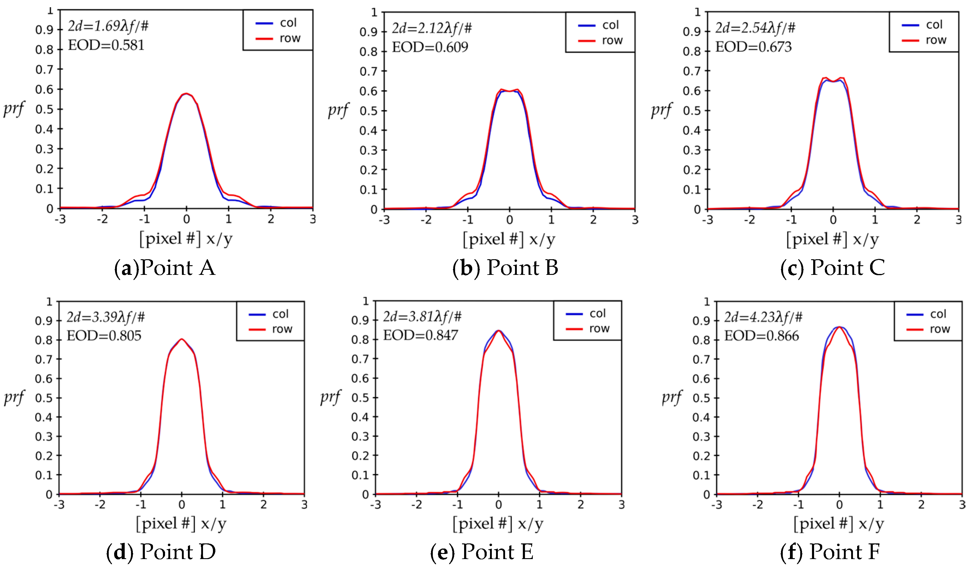
5.2. Aperture Configuration: Circular, Incorporating Rectangular Central Obscuration
Case 3: Small Pixel, Round Aperture with a Central Rectangular Obscuration
6. Discussion
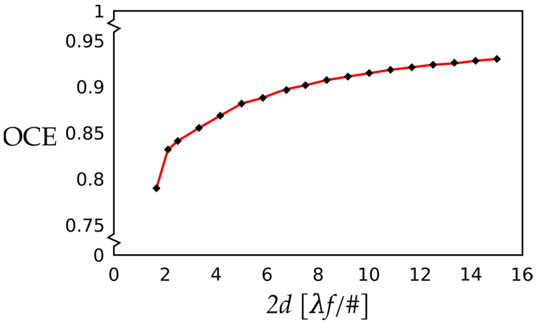
6.1. Signal-Carrying Energy on Detector
6.2. Small, Medium, and Large Pixels to Collect Signal-Carrying Energy
7. Summary and Conclusions
Author Contributions
Funding
Institutional Review Board Statement
Informed Consent Statement
Data Availability Statement
Acknowledgments
Conflicts of Interest
References
- Rauscher, B.J.; Fox, O.; Ferruit, P.; Ferruit, R.J.; Waczynski, A.; Wen, Y.; Xia-Serafino, W.; Xia-Serafino, B.; Alexander, D.; Brambora, C.; et al. Detectors for the James Webb Space Telescope Near-Infrared Spectrograph I: Readout Mode, Noise Model, and Calibration Considerations. arXiv 2007, arXiv:0706.2344. [Google Scholar] [CrossRef]
- Sutherland, W.; Emerson, J.; Dalton, G.; Atad-Ettedgui, E.; Beard, S.; Bennett, B.; Bezawada, N.; Born, A.; Caldwell, M.; Clark, P.; et al. The Visible and Infrared Survey Telescope for Astronomy (VISTA): Design, technical overview, and performance. Astron. Astrophys. 2015, 575, A25. [Google Scholar] [CrossRef] [Green Version]
- Scholl, M.S.; Wang, Y.; Randolph, J.E.; Ayon, J.A. Site certification imaging sensor for Mars exploration. Opt. Eng. 1991, 30, 590–597. [Google Scholar] [CrossRef]
- Scholl, M.S.; Padila, G.; Wang, Y. Design of a high resolution telescope for an Imaging sensor to characterize a (Martian) landing-site. Opt. Eng. 1995, 34, 3222–3228. [Google Scholar] [CrossRef]
- Scholl, M.S.; Padila, G. Push-broom reconnaissance camera with time expansion for a (Martian) landing-site certification. Opt. Eng. 1997, 36, 566–573. [Google Scholar] [CrossRef]
- Goodman, J.W. Introduction to Fourier Optics; McGraw-Hill: San Francisco, CA, USA, 1968; p. 141. [Google Scholar]
- Gaskill, J.D. Linear Systems, Fourier Transforms, and Optics; John Wiley & Sons: New York, NY, USA, 1978; p. 449. [Google Scholar]
- Strojnik, M. Point spread function of (multiple) Bracewell interferometric configuration(s) and the nulling hypothesis in planet detection. J. Appl. Remote Sens. 2014, 8, 084981. [Google Scholar] [CrossRef]
- Wolfe, W.L. Radiometric terms. In The Infrared Handbook, rev. ed.; IRIA, Ed.; ERIM for Office of Naval Research: Ann Arbor, MI, USA, 1993. [Google Scholar]
- Wolfe, W.L. Introduction to Infrared System Design; SPIE: Bellingham, WA, USA, 1996; Volume TT24, p. 17. [Google Scholar]
- Strojnik, M.; Scholl, M.K. Radiometry. In Advanced Optical Instruments and Techniques; Malacara, D., Thompso, B.N., Eds.; CRC Press: New York, NY, USA, 2018; pp. 459–717. ISBN 9781498720670. [Google Scholar]
- Kingslake, R. Lens Design Fundamentals; Academic Press: New York, NY, USA, 1978; p. 153. [Google Scholar]
- Fisher, R.; Tadic-Galeb, B. Optical System Design; McGraw-Hill: New York, NY, USA, 2000; p. 7. [Google Scholar]
- Smith, W. Modern Optical Engineering, 4th ed.; McGraw Hill: New York, NY, USA, 2008; p. 191. [Google Scholar]
- Hecht, E. Optics, 4th ed.; Addison Wesley: San Francisco, CA, USA, 2002; p. 470. [Google Scholar]
- Mahajan, V. Aberration Theory Made Simple; SPIE: Bellingham, WA, USA, 1991; Volume TT6, p. 71. [Google Scholar]
- Beyer, L.M.; Cobb, S.H.; Clune, L.C. Ensquared power for obscured circular pupils with off-center imaging. Appl. Opt. 1991, 30, 3569. [Google Scholar] [CrossRef] [PubMed]
- Harvey, J.E.; Ftaclas, C. Diffraction effects of telescope secondary mirror spiders on varies image-quality criteria. Appl. Opt. 1995, 34, 6337. [Google Scholar] [CrossRef] [PubMed]
- Barhydt, H. Effect of F/number and other parameters on performance of nearly BLIP search and surveillance systems. Opt. Eng. 1978, 17, SR-28. [Google Scholar]
- Barhydt, H. Figures of Merit for Infrared Sensors; SPIE: Bellingham, WA, USA, 1979; Volume 197, p. 64. [Google Scholar]
- Lloyd, J.M. Fundamentals of electro-optical imaging systems analysis. Electro-optical systems design, analysis, and testing. In The Infrared & Electro-Optical Systems Handbook; Accetta, J.S., Shumaker, D.L., Dudzik, M., Eds.; ERIM: Ann Arbor, MI, USA; SPIE: Bellingham, WA, USA, 1993; Volume 4, p. 18. [Google Scholar]
- Holst, G. Electro-Optical Imaging System Performance, 3rd ed.; SPIE: Bellingham, WA, USA, 2002; p. 204. [Google Scholar]
- Born, M.; Wolf, E. Principles of Optics, 7th ed.; Cambridge U. Press: Cambridge, UK, 1999; p. 443. [Google Scholar]
- Hudson, R.D. Infrared System Engineering; Wiley & Son: New York, NY, USA, 1969; pp. 270–429. [Google Scholar]
- Lloyd, J.M. Thermal Imaging Systems; Plenum Press: New York, NY, USA, 1975; pp. 11–166. [Google Scholar]
- Stoltzmann, D.E. The perfect point spread function. In Applied Optics and Optical Engineering; Shannon, R.R., Wyant, J.C., Eds.; Academic Press: New York, NY, USA, 1983; Volume IX, pp. 111–148. [Google Scholar]
- Wyant, J.C.; Creath, K. Basic wavefront aberration theory for optical metrology. In Applied Optics and Optical Engineering; Shannon, R.R., Wyant, J.C., Eds.; Academic Press: New York, NY, USA, 1992; Volume XI, pp. 1–53. [Google Scholar]
- Welford, W.T. Aberrations of the Symmetrical Optical System; Academic Press: London, UK, 1974; p. 22. [Google Scholar]


| Point on Figure 9 | 2d [λF#] | EOD from Figure 10 | OCE from Figure 9 | OCE × EOD |
|---|---|---|---|---|
| A | 1.69 | 0.581 | 0.864 | 0.502 |
| B | 2.12 | 0.609 | 0.922 | 0.561 |
| C | 2.54 | 0.673 | 0.901 | 0.606 |
| D | 3.39 | 0.805 | 0.836 | 0.673 |
| E | 3.81 | 0.847 | 0.820 | 0.694 |
| F | 4.23 | 0.866 | 0.825 | 0.714 |
Disclaimer/Publisher’s Note: The statements, opinions and data contained in all publications are solely those of the individual author(s) and contributor(s) and not of MDPI and/or the editor(s). MDPI and/or the editor(s) disclaim responsibility for any injury to people or property resulting from any ideas, methods, instructions or products referred to in the content. |
© 2023 by the authors. Licensee MDPI, Basel, Switzerland. This article is an open access article distributed under the terms and conditions of the Creative Commons Attribution (CC BY) license (https://creativecommons.org/licenses/by/4.0/).
Share and Cite
Strojnik, M.; Bravo-Medina, B.; Martin, R.; Wang, Y. Ensquared Energy and Optical Centroid Efficiency in Optical Sensors: Part 1, Theory. Photonics 2023, 10, 254. https://doi.org/10.3390/photonics10030254
Strojnik M, Bravo-Medina B, Martin R, Wang Y. Ensquared Energy and Optical Centroid Efficiency in Optical Sensors: Part 1, Theory. Photonics. 2023; 10(3):254. https://doi.org/10.3390/photonics10030254
Chicago/Turabian StyleStrojnik, Marija, Beethoven Bravo-Medina, Robert Martin, and Yaujen Wang. 2023. "Ensquared Energy and Optical Centroid Efficiency in Optical Sensors: Part 1, Theory" Photonics 10, no. 3: 254. https://doi.org/10.3390/photonics10030254