Article

Noise Considerations for Tomographic Reconstruction of Single-Projection Digital Holographic Interferometry-Based Radiation Dosimetry

1
School of Physical and Chemical Sciences, University of Canterbury, Christchurch 8041, New Zealand
2
Medical Physics and Bioengineering, Christchurch Hospital, 2 Riccarton Avenue, Christchurch 8011, New Zealand
3
Department of Radiation Oncology, University of Washington Medical Center (UWMC), Seattle, WA 98195, USA
4
Department of Radiation Oncology, Fred Hutchinson Cancer Center, Seattle, WA 98109, USA
*
Author to whom correspondence should be addressed.
Photonics 2023, 10(2), 188; https://doi.org/10.3390/photonics10020188
Submission received: 10 December 2022 / Revised: 22 January 2023 / Accepted: 2 February 2023 / Published: 9 February 2023
(This article belongs to the Special Issue Advances and Application of Imaging on Digital Holography)

Abstract

:
Optical Calorimetry (OC) is a 2D Digital Holographic Interferometry (DHI)-based measurement technique with potential applications for the 3D dosimetry of ultra-high dose rate (FLASH) radiation therapy beams through tomographic reconstruction. This application requires accurate measurements of DHI signals in environments with low signal-to-noise ratios (SNRs) in order to accurately measure absorbed energy to a medium per unit mass (Dose). However, tomographic reconstruction accuracy is sensitive to noise in the measurements. In this study, a virtual model of an OC dosimeter was used to characterize and model major sources of noise within a DHI setup, allowing for the modelled noise sources to be selectively reduced. The tomographic reconstruction of the 3D dose distribution was achieved using the inverse Abel transform. Reducing the noise contribution from atmospheric turbulence and mechanical vibration by one half improved the central axis reconstruction error from 6.5% to 1.3% and 1.1%, respectively, and the mean dose difference from 2.9% to 0.4% and 0.3%, respectively. This indicates the potential of the tomographic DHI-based 3D OC dosimeter to reconstruct accurate 3D dose distributions from a single projection if the specified sources of noise can be reduced to acceptable levels. The used methodology is applicable to any application of tomographic DHI where reconstruction quality is highly sensitive to noise.

1. Introduction

Optical interferometry is an established measurement technique where two interfering light waves are used to determine phase variations within a medium through the analysis of the resulting interference patterns or interferograms [1]. Digital Holographic Interferometry (DHI) is a specialized form of optical interferometry where the digital re-illumination of the interference patterns for different states of the medium allows for the reconstruction of two-dimensional maps of the phase change between the states with a subwavelength resolution [2,3]. This results in a highly sensitive and non-invasive measurement technique, with applications for measurement within the micro- to nano-meter scale; as such, it can be used to investigate phenomena such as small-scale mechanical displacements, surface deformations, vibrations, and refractive index changes [4,5].
DHI tomography refers to the reconstruction of three-dimensional (3D) datasets from the measurement of two-dimensional (2D) projections with a DHI setup. DHI tomography is predominantly suited for high signal-to-noise ratio (SNR) applications, such as flame and plasma flume imaging or dynamic temperature fields in liquids and gases [4,6]. For low-SNR environments, the relative impact of the various sources of noise within the measurement system are more pronounced and have a greater impact on the resulting measurement accuracy. It is against this background that we present an approach where we investigate the impact of different sources of noise on the resulting measurement accuracy with the aim to identify key areas for improvement within the DHI measurement system.
To aid the development and refinement of DHI measurement systems, the virtual simulation of the DHI system can be used to determine how various design parameters and system noise influence measurement accuracy. For example, Hubley et al. (2019) [7] used a virtual model to successfully investigate, implement and validate improvements to a physical DHI-based Optical Calorimetry (OC) [8] measurement system. Significant work was undertaken to first ensure that the calibration of each optical component within the virtual model was accurate and then to validate the accuracy of the virtual model with an experimental set-up [7,9,10]. This virtual interferometer model has subsequently been used to investigate the impact of environmental parameters on reconstruction accuracy, as well as modelling and validating design changes [7]. An advantage of having a virtual model of an interferometer with well-characterized sources of noise is that it is representative of the noise present in a real-world DHI measurement system. This facilitates investigation into identifying which aspects of the DHI system require the most attention in terms of reducing noise to achieve the greatest increase in performance.
A potential biomedical application of tomographic DHI when the SNR is low is in the field of radiation dosimetry, i.e., the measurement of the ionizing radiation clinically used to deliver radiation therapy. The quantity of interest in radiation dosimetry is absorbed dose D , defined as the mean energy d ε ¯ imparted to a medium of mass d m by ionizing radiation
D = d ε ¯ d m     Gy ,
measured in units of Gray (Gy).
Radiation therapy is recommended for approximately 50% of cancer patients during the course of their illness [11]. A highly promising field of research within radiation therapy is FLASH therapy [12,13]. This is an emerging treatment approach that uses ultra-high dose rate (UHDR) beams with dose rates in excess of 40 Gy/s, which have shown improved treatment outcomes with reduced side-effects [14]. However, these novel beams have proven difficult to accurately measure with traditional ionometric measurement techniques [15,16,17]. There is therefore a need to develop new dosimetry approaches to accurately quantify the dose in FLASH beams.
A DHI-based Optical Calorimetry dosimeter, such as the prototype developed by Cavan and Meyer [8], has the potential to overcome several inherent challenges in FLASH dosimetry [18]. Unlike many traditional measurement techniques, the measured signal is dose-rate-independent, it directly rather than indirectly measures the dose-to-water ratio, and all parts of the dosimeter are located outside the radiation beam, thus avoiding the perturbation of the radiation beam by the detector itself. As a result, correction factors for dose rate dependence, beam perturbation, and dose-to-water conversions (each of which contribute to measurement uncertainty) are not required. None of these dependencies are well-established in FLASH dosimetry [12,15,16,17], and no national standards exist. Therefore, avoiding the need to characterize these factors will reduce the uncertainty in FLASH dosimetry measurements and assist in the acceptance of FLASH therapy for clinical use.
Another advantage of OC dosimetry is that it lends itself well to obtaining spatially resolved information about a radiation beam. Typical OC dosimeter output is a single 2D projection of the absorbed radiation energy deposited in a medium along the optical path of the probing laser [7,8]. As the absorbed energy is proportional to the dose, it enables the possibility of producing a 3D dose distribution through the process of tomographic reconstruction. A 3D OC dosimeter could provide distinct advantages over traditional dose-to-a-point-based measurement approaches.
A tomographic reconstruction generally requires multiple projections from a range of angles. Acquiring these projections with a DHI setup is likely to be difficult to achieve due to the complex arrangement of optical components within a DHI setup and the sensitivity to additional noise in a low-SNR dosimetry environment. Therefore, the additional mechanical complexity introduced by modifying the current OC dosimeter to be able to capture multiple projections would likely negate any image reconstruction improvements [6]. However, when feasible, there is significant motivation to perform a tomographic reconstruction only using a single projection. For the measurement of radially symmetric distributions, this can be achieved, for example, by means of the inverse Abel transform [19]. The suitability of the inverse Abel transform for the 3D reconstruction of FLASH radiation therapy beams was demonstrated by Ashraf et al. (2021) [20]. However, this was for a radioluminescence imaging application rather than OC.
One of the challenges in radiation dosimetry with DHI is the very low magnitude signals comprising a dose measurement. The principle of operation is detailed below in the methods section, but in summary, the radiation beam energy absorbed in a medium is converted into heat, which results in refractive index changed proportional to the dose. For example, the temperature changes due to the energy deposited by a typical daily treatment dose of 2 Gy of radiation into a volume of water is on the order of two one-thousandths of a degree Celsius [21,22]. This differs from a number of more typical DHI applications, such as the measurement of 3D temperature fields in liquids, where measurements are made with a temperature difference in the order of 10 °C [6]. The orders of magnitude lower signals in radiation dosimetry decrease the SNRs of dosimetry measurements, thereby increasing the influence of noise on measurement accuracy. Consequently, this impacts the accuracy of the tomographic reconstruction of a dose. A tomographic DHI approach using the inverse Abel transform was used by Vaziri et al. (2020) [23] for the measurement of Monte Carlo (MC)-modelled electron beams. Gaussian noise was added to model the measurement noise, resulting in a reconstructed dose distribution with a mean uncertainty of 14 Gy [23].
Our approach is different and based on the virtual model developed by Hubley et al. [7]. It has been experimentally validated and offers the possibility to expand upon the simple noise model by Vaziri et al. [23] by using several realistic noise components that impact the DHI system and by being able to systematically vary the levels of noise to investigate any correlation between reconstruction sensitivity and the noise component and level.
There are a number of additional factors that affect the absolute accuracy of a DHI dose measurement, such as phase unwrapping, temperature-to-refractive-index conversion, laser heating, and speckle scatter. The effects of these errors on tomographic reconstruction accuracy are generally smaller than the effect of noise in the projection data, and they were beyond the scope of this work. As such, the aim of this work was to investigate the relative impact that various sources of noise within our DHI-based Optical Calorimeter had on the accuracy of an inverse Abel tomographic reconstruction applied to a single projection. While this approach is generic for low-SNR applications, here, it was applied to a realistic 70 MeV proton FLASH beam in order to guide the development and refinement of a 3D DHI OC dosimeter.

2. Materials and Methods

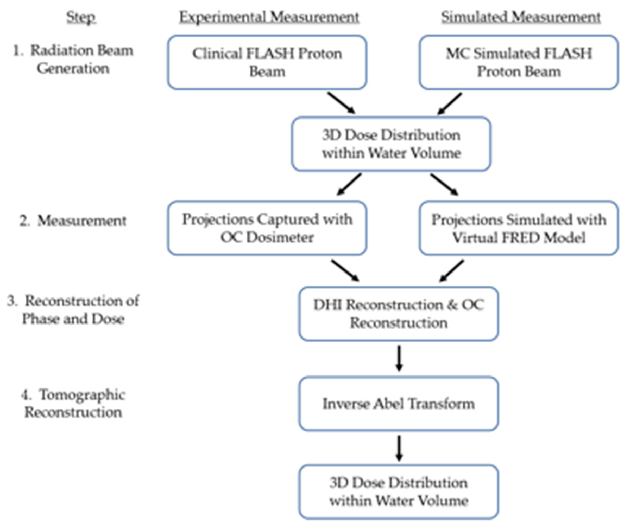
2.1. Data Generation and Workflow

This work assessed the impact of noise on single-projection tomographic DHI reconstruction. Figure 1 shows an overview of the steps performed when taking an experimental measurement and the simulation pathway used to model the experimental measurements.
The ground truth 3D dose distribution data (Step 1) were obtained via Monte Carlo simulation using TOPAS (Tool for Particle Simulation), a Geant4-based particle transport toolkit used for numerous dosimetric applications [24,25]. The dose distribution in a volume of water from a 70 MeV proton beam, with a circular aperture 40 mm in diameter at a distance of 40 mm from the surface of the water, was modelled. Output was scored onto a 1003 grid with a voxel size of 0.5 mm3 before being interpolated to 2563 with a voxel size of 0.2 mm3. These dimensions were chosen as a reasonable compromise between the computationally expensive Monte Carlo simulation and the maintenance of spatial resolution, so the dose distribution remained smooth at spatial scales of one millimeter. To characterize the simulated dose distributions, two clinical dosimetric metrics common to radiation physics were used, namely, the Central Axis (CAX) Percentage Depth Dose (PDD) and lateral profiles [26,27]. The PDD is the relative dose at each depth along the center of the distribution normalized to the maximum dose and expressed as a percentage, and profiles are comprised of the dose at each point laterally through a distribution at the depth of dose maximum (Dmax) normalized to the maximum dose.
The used OC dosimeter was based on the simple holographic interferometer design outlined in Figure 2. A detailed description of this interferometer is given in [7,8], but a summary is provided here. A coherent HeNe laser is split into an object and reference beam, with the object beam probing a test cell containing a volume of water while the reference beam only passes through air. The radiation beam to be measured impinges on the test cell orthogonal to the plane of the OC system and deposits energy into the test cell along its beam path, thereby causing a temperature change that results in refractive index changes. The refractive index changes of the water within the test cell results in the object beam traversing a longer Optical Path Length (OPL), thus causing relative phase changes between the object and reference beams when recombined at the detector. This phase difference causes an interference pattern, called an optical interferogram, that is captured by the CMOS detector. Analogous to standard holographic interferometry techniques in which the image is viewed via illumination, these interferograms can be digitally “re-illuminated” [3] by the reference wave, creating a digital image of the object wave or a digital hologram. This reconstructs the phase and amplitude information of the object wave. For interferograms produced by holographic interferometry, the Fresnel transform is used to calculate the phase difference between the object and reference waves from reconstructed fringe patterns.
As the water is irradiated with a beam of radiation, OC captures interferograms at multiple states of the volume of water. A DHI algorithm is used to extract the relative difference in phase change between images of both the irradiated and un-irradiated states. This produces a 2D map of the integrated phase change between the two states. The 2D map of the phase change is then related to the change in optical path length, refractive index and temperature, from which the integrated absorbed dose can be determined. This process is illustrated in Figure 3, and full details of this conversion process can be found in [7,8]. The result is a 2D map of the dose integrated across the width of the test cell [8], completing Step 3 of Figure 1.
The measurement of the 3D dose distribution within the test cell of the DHI-based OC dosimeter was simulated with FRED (Photon Engineering, Tucson, AZ, USA) [28], the simulated measurement side of Step 2 within Figure 1. FRED is a commercially available optical engineering software utilizing complex ray tracing to model optical systems. In complex ray tracing, free space propagation is modelled using conventional electromagnetic field equations. The electromagnetic field distribution is converted into a basis set of small Gaussian beamlets. These beamlets are then considered rays at any optical interface. The FLASH proton beam 3D dose distributions were exported to FRED as a cube of 1 mm voxels of varying refractive indexes, with the change in the refractive index distribution proportional to the distribution of the dose. The virtual dosimeter model was used to ray-trace the object beam through each individual voxel of the water volume, calculating the integrated phase change of the object beam as it passed through the dose distribution and producing the virtual optical interferograms. The same DHI reconstruction to determine phase change and calculated dose was performed, generating the virtual 2D map of the integrated dose. The method described above can measure a 50 milliradian phase shift, corresponding to a typical daily treatment dose of 2 Gy, with a type A, k = 1 uncertainty of 5.6% [10].
An additional capability of the interferometer model in FRED is the ability to characterize and vary the impact of different sources of noise within the OC dosimeter. Previous work on OC dosimeter refinement using FRED characterized several sources within the measurement system, including atmospheric turbulence and mechanical vibration [7]. Atmospheric turbulence refers to short timescale fluctuations in atmospheric temperature, pressure, and humidity within the interferometer arrangement. By dividing the space within the interferometer into small voxels and simulating small random fluctuations in the temperature, pressure, and humidity within reasonable operational ranges, the refractive index of the air between the interferometer components can be realistically varied and its impact on measurements can be determined. Mechanical vibrations refer to beamline length changes resulting from the local displacements of optical components. This vibration can be simulated by displacing each component a random distance from its zero position up to a maximum displacement determined by the amplitude of the modelled vibration. Further details on the virtual modelling and characterization of these noise sources and their experimental validation can be found in [7].
The amount of noise present in the simulated DHI measurement system can be adjusted as required, allowing for an analysis of how the noise effects reconstruction accuracy. For this study, the OC dosimeter output was simulated for the following levels of noise modelled in the virtual dosimeter:
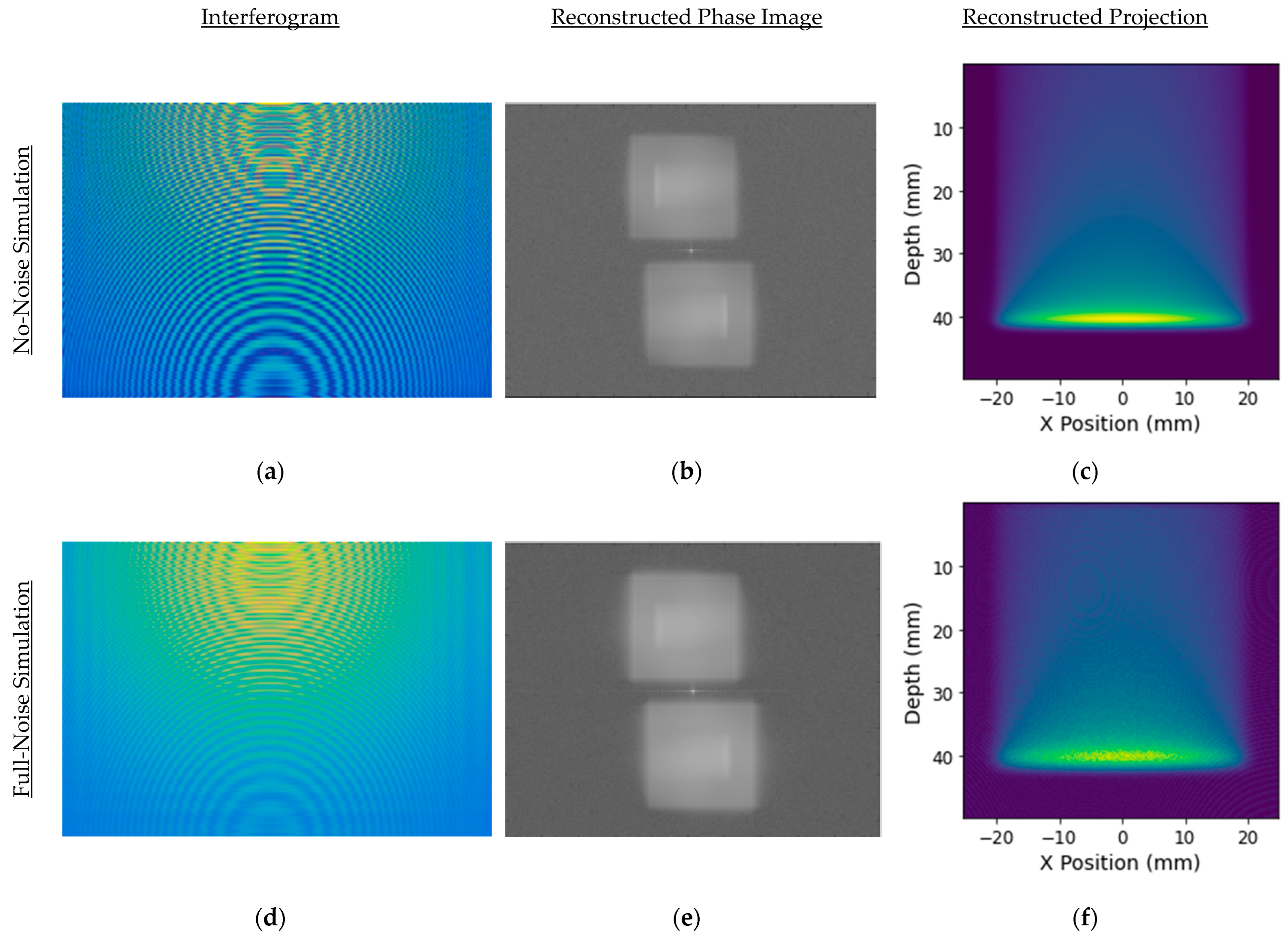
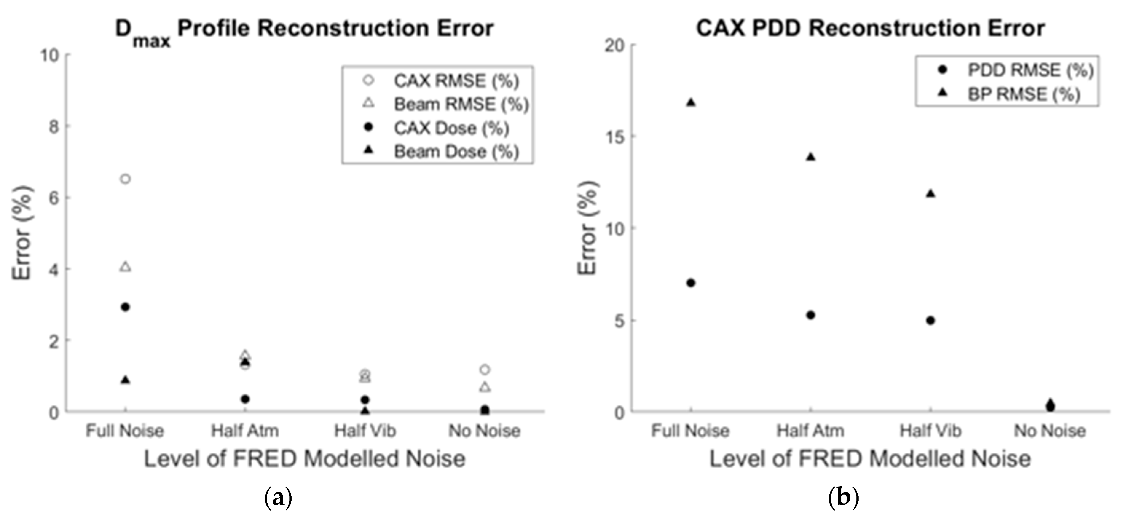
  • No-noise simulation—the theoretical best level of performance, where no information is lost due to the modelled sources of noise within the dosimeter. Interferograms were generated by the virtual OC dosimeter with the modelled refractive index distribution within the water cell perturbed based on the MC-simulated dose distribution, and the noise contribution due to atmospheric turbulence and mechanical vibration within the DHI measurement system was removed.
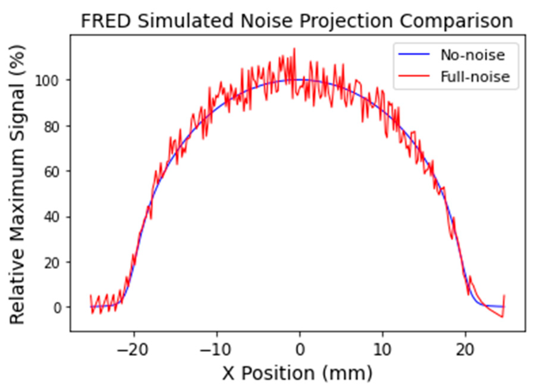
  • Full-noise simulation—representing the current level of dosimeter performance. Interferograms were generated by the virtual OC dosimeter as for the no-noise simulation, but the full noise contribution due to atmospheric turbulence and mechanical vibration within the DHI measurement system was modelled.
  • Reduced atmospheric turbulence simulation—interferograms were generated as for the full-noise simulation, but the noise contribution from the modelled atmospheric turbulence was reduced to half the maximum level by reducing the range of the temperature, pressure, and humidity fluctuations by half.
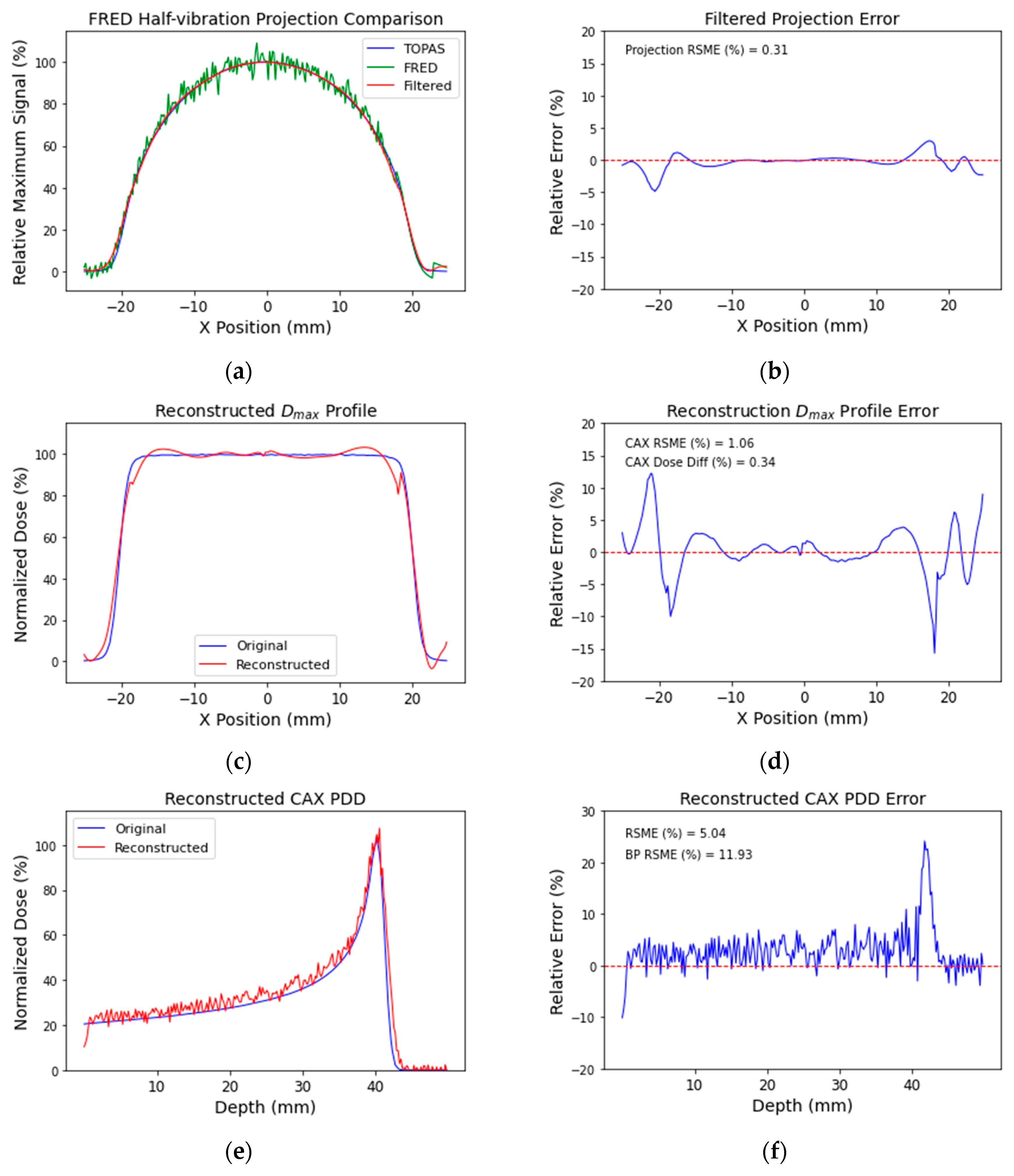
  • Reduced mechanical vibration simulation—interferograms were generated as for the full-noise simulation, but the noise contribution from the modelled mechanical vibration was reduced to half the maximum level by reducing the maximum amplitude of the vibrations by half.
In Step 4, the 3D dose distribution was tomographically reconstructed using the inverse Abel transform [19], implemented using the PyAbel package within Python [29,30]. The inverse Abel transform is a mathematical integral transform that is used in the analysis of spherically or cylindrically symmetric functions. Prior to reconstruction, a Gaussian filter was applied to the projection data to reduce the impact of the noise inherent to the measurement process on the reconstruction accuracy. To reduce the impact of the random component of the modelled noise, each simulation for a particular level of noise was repeated four times, each with a different state of the random modelled noise, and then the average was taken. Four samples were chosen as a compromise between increasing the spatial resolution and degrading the temporal resolution of an experimental measurement.

2.2. Data Analysis

To evaluate the reconstruction accuracy, reconstructed profiles at depths corresponding to the depth of maximum dose, Dmax, and CAX PDDs were compared to the equivalent points within the original TOPAS distribution. To quantify the impact on accuracy, two metrics were used. The Root Mean Square Error (RMSE) between the original value x and the reconstructed value y for each point N along the respective PDD or profile
R M S E = n = 1 N x n y n 2 N   ,
and the percentage dose difference Δ D % between the mean dose within a specified region of the original x and reconstructed profiles y for a specified region
Δ D % = y = x ¯ x ¯ 100   .
The comparison was performed in two regions for the profiles, the CAX (defined as the central 21 pixels) and the beam region (defined as the central 121 pixels), to provide clinically relevant dosimetry information. The PDDs were analyzed over the whole distribution and the Bragg Peak (BP) region (defined as a region of 21 pixels centered upon the depth of Dmax), as this area is of particular interest for clinical proton dosimetry. These regions are displayed on the profiles and PDDs in Figure 4. The reconstructed distributions were then compared with the original MC 3D dose distribution to determine the reconstruction accuracy.
Additionally, the magnitude of noise within each projection was quantified. The MC 3D distribution was summed in one dimension, representing the perfect integration of the projection with zero information lost to noise. The difference between this projection and the FRED projection for the beam region at the depth of Dmax was determined, and then the RMSE of the difference was calculated. This value is defined as the RMSE (%) of the Projection Error, and we used it to compare the variability in the projections for each level of modelled noise with a single number.

3. Results

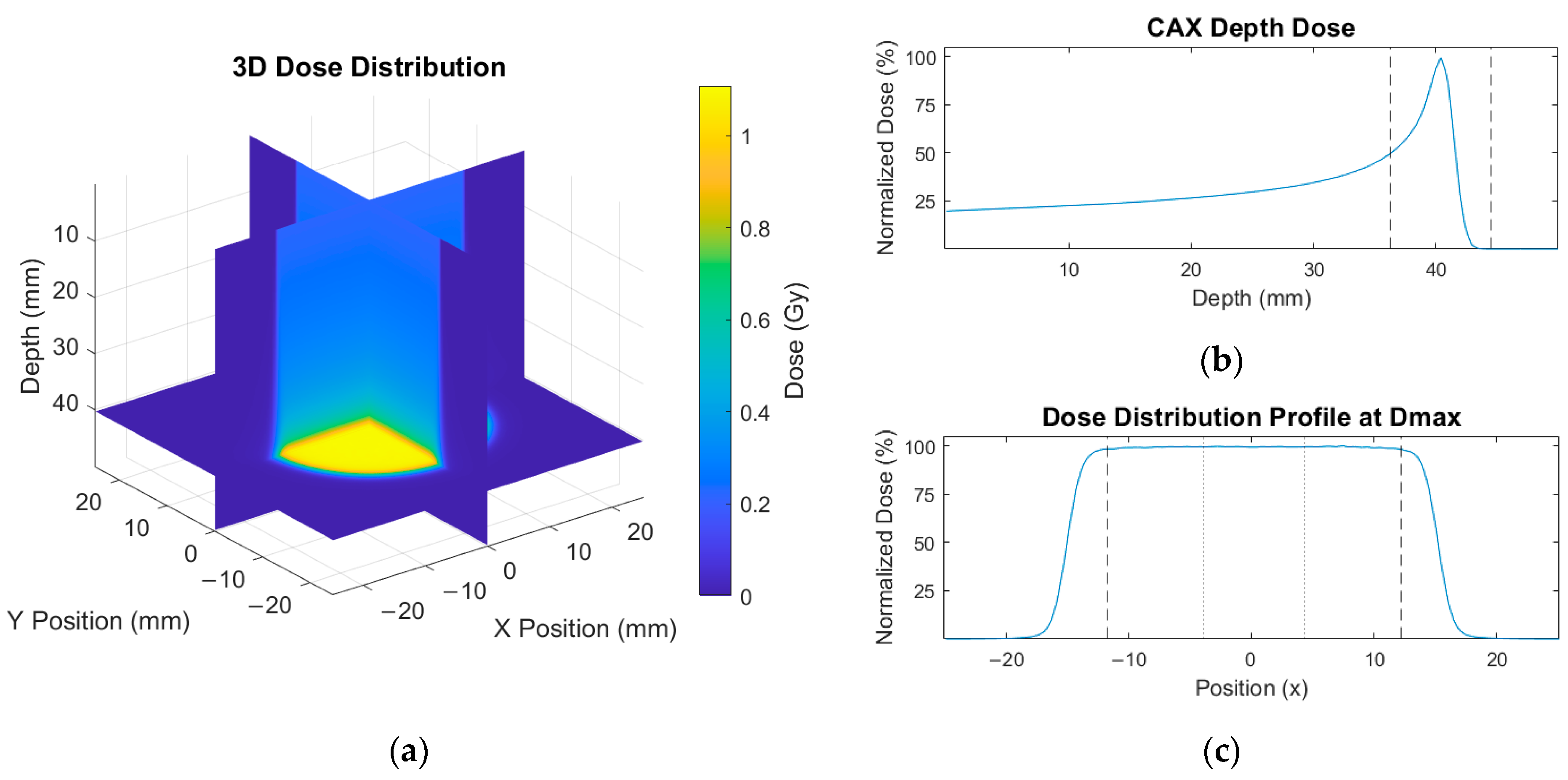
3.1. Beam Data Simulation

An example of the Monte Carlo-simulated proton beams generated in TOPAS is shown in Figure 4. In Figure 4a, the proton beam vertically enters the water cell from the top, depositing the dose along its beam path. The dose is normalized at a depth of 41 mm at the Bragg Peak, with the entrance dose of approximately 23%. The resulting CAX PDD generated from the 3D distribution is shown in (b), and the Dmax profile is shown in (c). To ensure low statistical uncertainty, 1 billion primary photons were generated for these simulations, with a standard error of less than 0.3% for all produced beam models.

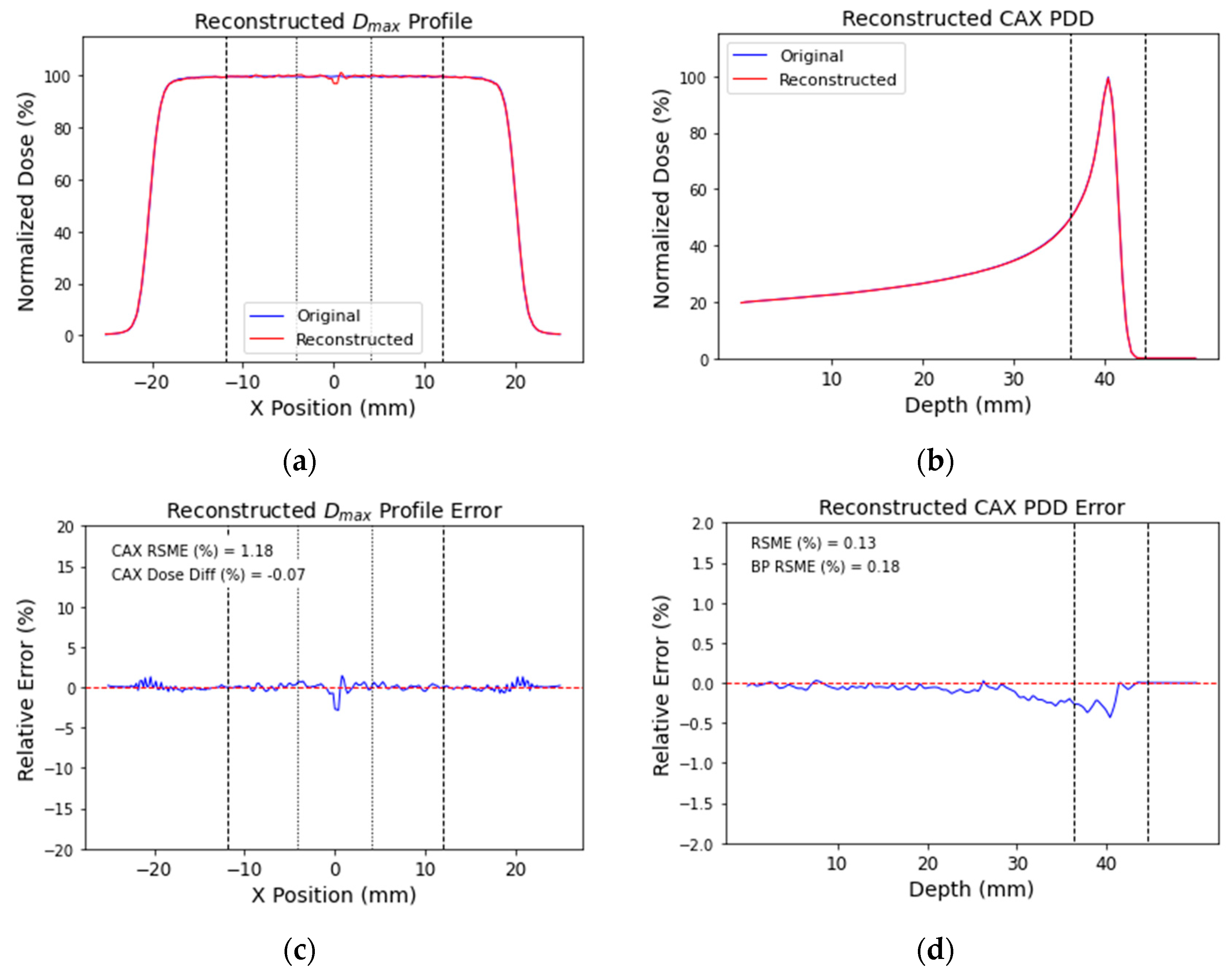
3.2. No-Noise Simulation Reconstruction

The initial accuracy of the tomographic reconstruction was tested using reconstructed interferograms generated by the virtual OC dosimeter using the no-noise simulation. The reconstruction of the no-noise FRED data indicated the degradation of reconstruction accuracy due to loss of information in the DHI process, such as phase unwrapping or refractive-index-to-temperature conversion. The interferogram generated in FRED for the no-noise simulation is shown in Figure 5a for illustration. The reconstructed projection (Figure 5c) was generated from the reconstructed phase image (Figure 5b) by cropping out one of the twin images, rotating it 90 degrees, and normalizing it to 100% at the maximum signal.
Table 1 displays the tomographic reconstruction accuracy achievable with both sources of noise removed from the virtual interferometer model. The inverse Abel transform reconstruction generated a profile RMSE of less than 1.2%, a PDD RMSE of less than 0.2%, and a mean dose difference of less than 0.1% for all analyzed regions. A Projection Error RMSE (%) of 0.03 indicated that the projection measured with the OC dosimeter accurately replicated the equivalent projection data generated from the MC-simulated proton beam dose distribution.
The reconstructed Dmax profile and PDD are shown in Figure 6, with the reconstructed dose well-matching the original at the beam edge and main portion of the radiation beam. A reconstruction artefact is present in the center of the profile, a result of the decreasing accuracy of the inverse Abel transform at points close to the axis of radial symmetry [29]. Due to the combination of this artefact and the location of the CAX PDD, this artefact was found to be present at all depths, so the PDD measurement at each depth were calculated over the central 21 pixels comprising the CAX region. This was considered a reasonable assumption due to the inherently flat and symmetric nature of clinical radiation beams [26].

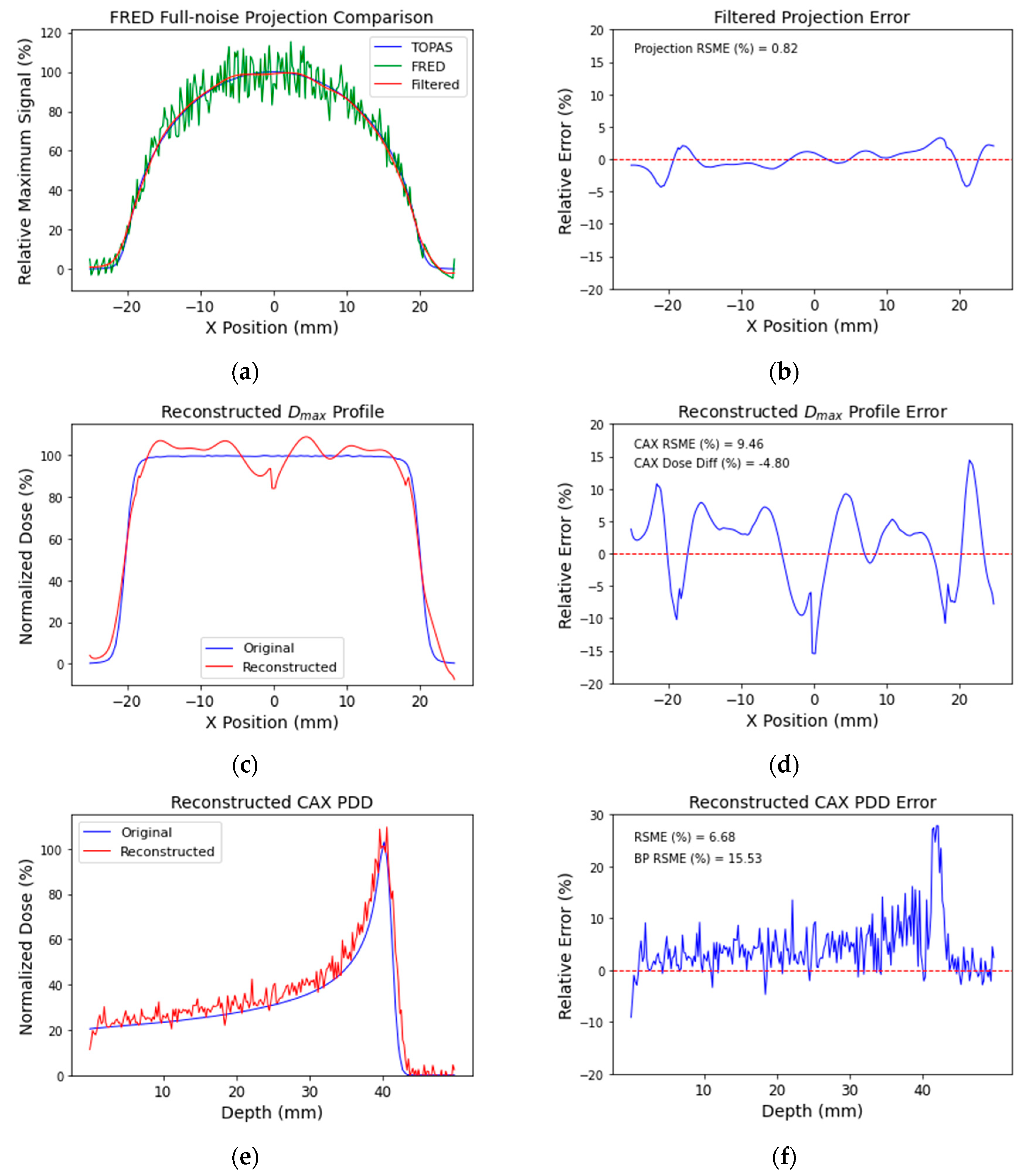
3.3. Full-Noise Simulation Reconstruction

The full-noise FRED simulation data indicated the level of performance of the DHI-based OC dosimeter. The interferograms generated in FRED from the full-noise simulation can be seen in Figure 5. When comparing the two, the blurring of the interference fringes is apparent, with these less well-defined in the full-noise interferogram. The reconstructed phase image shows the real and virtual twin images, along with the central DC term. These images show a similar trend, with a greater degree of blurring present in the full-noise simulation. Comparing the no-noise and full-noise projection images again showed a greater degree of blurring in the full-noise projection, with this most clearly seen at the depth of the Bragg Peak. The increase in noise between the no-noise and full-noise simulations can be seen in the comparison of profiles through the projection data at the depth of Dmax (Figure 7).
Filtering applied prior to reconstruction removed much of this noise but was unable to exactly reproduce the original projection data (Figure 8a,b). The reconstruction of the full-noise projection data using the inverse Abel transform can be seen in Figure 8. The reconstructed profile shows a reasonable approximation of the general shape of the MC-generated profile and the estimation of the edge of the beam (Figure 8c), but the variability across the profile is noticeable, with errors of up to 15% (Figure 8d). For the PDD (Figure 8e), the presence of the CAX reconstruction artefact resulted in an increased reconstruction error, with the reconstructed distribution slightly overestimated. The increase in RMSE was most notable in the BP region (Figure 8f).
When the mean of the four full-noise simulations was calculated, the magnitude of the noise in the full-noise projection was reduced without being entirely eliminated. This indicates that while there were random components of the virtual noise models that contributed to the noise signal, which were reduced by averaging repeated measurements, there was also a systematic noise contribution that remained prevalent. The mean reconstruction accuracy metrics for the individual simulation reconstruction results, compared with the reconstruction results when the projections were averaged prior to reconstruction, are shown in Table 2.
Averaging the four projections prior to reconstruction resulted in a reduction in the magnitude of noise in the projection data, indicated by the approximately 30% reduction in the Projection Error RMSE for the averaged projection compared with the mean of the single-simulation results. This corresponded with an increase in the reconstruction accuracy, as shown by the approximately 40% reduction in the Dmax Profile RMSE for both the beam and CAX regions of the profile. Negligible changes were observed for the PDD RMSE results. The mean dose difference results also remained unchanged, indicating that averaging prior to reconstruction reduced the noise without altering the final reconstructed dose values. As this technique improved the quality of the reconstruction, it was used for all subsequent simulations.

3.4. Reduced Noise Simulation Reconstruction

To determine the relative impact of atmospheric turbulence and mechanical vibrations on the reconstruction accuracy, the interferometer was simulated in FRED with the modelled noise for one of the sources reduced to half the maximum level. An example of these results is shown in Figure 9 for the reduced mechanical vibration simulation. The filtered projection (Figure 9a,b) showed an improved match to the TOPAS projection (ground truth) in the central region and subsequently resulted in an improved profile at Dmax (Figure 9c,d) and CAX PDD (Figure 9e,f) reconstruction relative to the full-noise simulation. The CAX PDD still displayed a slight overestimation, but the magnitude of this error was reduced compared with the full-noise simulation.
When reconstruction accuracy metrics were compared for each level of simulated noise (Figure 10), a clear trend was seen. Reducing the atmospheric turbulence and mechanical vibration levels by half led to a considerable improvement over the full-noise simulation, with the half-vibration simulation producing slightly superior results compared with the half-atmospheric turbulence. The reconstruction accuracies of these simulations were comparable to the no-noise simulation for the RMSE in the profiles, though we did not obtain quite the same level of accuracy for the mean dose differences. The PDD contained slightly larger errors compared with the profiles but again showed an improvement with reduced noise.

4. Discussion

This work showcases an approach to assessing the impact of different sources of noise on the tomographic reconstruction accuracy of a single-projection DHI-based measurement system through the use of an experimentally validated virtual model [7].
The initial no-noise simulation, with the atmospheric turbulence and mechanical vibration noise sources removed, highlighted the potential accuracy of the inverse Abel transform in a low-noise environment. The reconstruction of the Monte Carlo 3D dose distribution showed a high accuracy for the profile and PDD reconstructions, with only a small reconstruction artefact in the center of the profile distribution. While the presence of this artefact was not desirable, as it limits the accuracy of the CAX dose reconstruction, it was not unexpected due to the decreasing accuracy of the inverse Abel transform as it approached the axis of radial symmetry [29]. The asymmetric nature of the artefact resulted in it averaging out when the mean of the central region was taken. These no-noise results indicate that the DHI-based 3D OC dosimeter is a promising method for the tomographic reconstruction of dose distributions.
The full-noise measurements are indicative of the existing levels of noise in existing OC dosimeter systems and highlights the challenges this noise provides for performing tomographic reconstructions in low-SNR environments. The most prominent reconstruction artefacts were found to occur at the CAX, exaggerating the decrease in the accuracy of the inverse Abel transform at the axis of radial symmetry, and at the beam edges, a consequence of the required heavy projection filtering that led to an inevitable loss of spatial resolution. The reconstructed PDDs showed a high degree of variability compared with the profiles, with the results in the Brag Peak region of the PDD reaching errors of greater than 15%. Part of this was due to the CAX PDD always containing the observed central reconstruction artefact, while the steep dose gradient within the Bragg Peak region resulted in an increased sensitivity to reconstruction errors. This can be clearly seen in the percentage error plot for Figure 9f, with the largest errors occurring at depths just beyond the Bragg Peak where the dose gradient was the greatest. These errors were similar in magnitude to those observed in [23].
When the noise contributions from the atmospheric turbulence and mechanical vibrations were reduced by half, large improvements to the tomographic reconstruction accuracy were observed. This accuracy increase indicates that potential performance improvements are achievable for the OC dosimeter and that investment into reducing the influence of mechanical vibration or atmospheric turbulence on the measurement system would considerably improve the clinical utility of DHI in radiation dosimetry. Of the two, reducing mechanical vibration showed a slightly greater improvement in reconstruction accuracy and should be the first area to investigate.
This work investigated the impact atmospheric and mechanical noise on tomographic reconstruction accuracy, as noise is the biggest contributor to the accuracy of reconstructed 3D dose distribution. Other factors contributing to the accuracy of dose measurements, such as phase unwrapping, temperature-to-refractive-index conversion, laser heating, and speckle scatter, were not investigated in this work because their relative contribution to the tomographic reconstruction accuracy are much less than noise in the projection data. Nevertheless, these factors remain areas of investigation for the OC dosimeter project team.
When DHI is performed in a laboratory setting, sources of noise such as atmospheric turbulence can be carefully controlled. In the application of DHI presented here, measurements were performed in clinical settings under much less controlled conditions, so improving the total system efficiency is critical. Our results show the difficulty of performing tomographic reconstruction with low-SNR measurements. Future measurements using a pulsed laser source may improve efficiency, but care must be taken when introducing a temporal delay between the object and reference beams. Quantifying a metric such as the ambiguity efficiency [31,32] would allow the performance of the system to be characterized as a function of the temporal delay, driving future improvements to the design.

5. Conclusions

3D Optical Calorimetry is a tomographic DHI technique that is currently limited in low-SNR environments such as during radiation dosimetry. This is due to the high sensitivity of a single-projection inverse Abel transform reconstruction to noise. A previously experimentally validated virtual model of an OC radiation dosimeter was used to simulate a DHI system, with varying levels of noise from known sources applied. Reducing the magnitude of these individual sources of noise allowed for the analysis of how accurate DHI tomographic reconstruction was when different types and amounts of noise were present. Reducing noise contributions from atmospheric turbulence and mechanical vibration improved the reconstruction accuracy from a CAX RMSE of 6.5% and CAX dose difference of 2.9% for the full noise simulation to 1.3% and 0.4% for atmospheric turbulence and 1.1% and 0.3% for mechanical vibration, respectively.
These results show that the DHI-based OC dosimeter could be used to reconstruct a full three-dimensional dose distribution with clinically acceptable accuracy, provided that future improvements to the current prototype that reduce the influence of atmospheric turbulence and mechanical vibration are made. This presents a potential alternative solution for the dosimetry of FLASH proton beams.
While this approach was directed towards radiation dosimetry in ultra-high dose rate FLASH therapy beams, the methodology presented in this paper is applicable to any application of tomographic DHI where noise impacts the reconstruction quality.

Author Contributions

The listed authors’ contributions to this work are as follows: conceptualization, T.T., J.R., A.M., J.M. and S.M.; methodology, T.T., J.R. and S.M.; software, T.T. and J.R.; validation, T.T.; formal analysis, T.T. and S.M.; investigation, T.T.; resources, S.M.; data curation, T.T.; writing—original draft preparation, T.T.; writing—review and editing, T.T., A.M., J.M. and S.M.; visualization, T.T.; supervision, A.M., J.M. and S.M.; project administration, A.M., J.M. and S.M. All authors have read and agreed to the published version of the manuscript.

Funding

This research received no external funding.

Institutional Review Board Statement

Not applicable.

Informed Consent Statement

Not applicable.

Data Availability Statement

The data presented in this study are available from the corresponding author upon reasonable request.

Conflicts of Interest

The authors declare no conflict of interest.

References

  1. Hariharan, P. Optical interferometry. Rep. Prog. Phys. 1991, 54, 339–390. [Google Scholar]
  2. Schnars, U.; Jüptner, W.P.O. Digital recording and reconstruction of holograms in hologram interferometry and shearography. Appl. Opt. 1994, 33, 4373. [Google Scholar] [CrossRef] [PubMed]
  3. Schnars, U.; Jueptner, W. Digital Holography; Springer: Berlin/Heidelberg, Germany, 2005. [Google Scholar]
  4. Petrov, V.; Pogoda, A.; Sementin, V.; Sevryugin, A.; Shalymov, E.; Venediktov, D.; Venediktov, V. Advances in Digital Holographic Interferometry. J. Imaging 2022, 8, 196. [Google Scholar] [CrossRef] [PubMed]
  5. Hernández-Montes, M.d.S.; Mendoza-Santoyo, F.; Flores Moreno, M.; de la Torre-Ibarra, M.; Silva Acosta, L.; Palacios-Ortega, N. Macro to nano specimen measurements using photons and electrons with digital holographic interferometry: A review. J. Eur. Opt. Soc. Rapid Publ. 2020, 16, 16. [Google Scholar] [CrossRef]
  6. Cubreli, G.; Psota, P.; Dančová, P.; Lédl, V.; Vít, T. Digital Holographic Interferometry for the Measurement of Symmetrical Temperature Fields in Liquids. Photonics 2021, 8, 200. [Google Scholar] [CrossRef]
  7. Hubley, L.; Roberts, J.; Meyer, J.; Moggré, A.; Marsh, S. Optical-radiation-calorimeter refinement by virtual-sensitivity analysis. Sensors 2019, 19, 1167. [Google Scholar] [CrossRef] [PubMed]
  8. Cavan, A.; Meyer, J. Digital holographic interferometry: A novel optical calorimetry technique for radiation dosimetry. Med. Phys. 2014, 41, 022102. [Google Scholar] [CrossRef]
  9. Roberts, J.; Moggré, A.; Marsh, S.; Meyer, J. Optical Calorimetry for Radiation Dosimetry. In Proceedings of NZPEM, Hamilton, New Zealand, 9 March 2020. [Google Scholar]
  10. Roberts, J.; Moggré, A.; Marsh, S.; Juergen, M. Optical Calorimetry for Radiation Dosimetry. In Proceedings of AAPM|COMP, Virtual Meeting, 12–16 July 2020. [Google Scholar]
  11. Delaney, G.; Jacob, S.; Featherstone, C.; Barton, M. The role of radiotherapy in cancer treatment: Estimating optimal utilization from a review of evidence-based clinical guidelines. Cancer 2005, 104, 1129–1137. [Google Scholar] [CrossRef]
  12. Esplen, N.; Mendonca, M.S.; Bazalova-Carter, M. Physics and biology of ultrahigh dose-rate (FLASH) radiotherapy: A topical review. Phys. Med. Biol. 2020, 65, 23TR03. [Google Scholar] [CrossRef]
  13. Favaudon, V.; Caplier, L.; Monceau, V.; Pouzoulet, F.; Sayarath, M.; Fouillade, C.; Poupon, M.F.; Brito, I.; Hupé, P.; Bourhis, J.; et al. Ultrahigh dose-rate FLASH irradiation increases the differential response between normal and tumor tissue in mice. Sci. Transl. Med. 2014, 6, 245ra93. [Google Scholar] [CrossRef]
  14. Bourhis, J.; Sozzi, W.J.; Jorge, P.G.; Gaide, O.; Bailat, C.; Duclos, F.; Patin, D.; Özşahin, M.; Bochud, F.; Germond, J.F.; et al. Treatment of a first patient with FLASH-radiotherapy. Radiother. Oncol. 2019, 139, 18–22. [Google Scholar] [CrossRef]
  15. Romano, F.; Bailat, C.; Jorge, P.G.; Lerch, M.L.F.; Darafsheh, A. Ultra-high dose rate dosimetry: Challenges and opportunities for FLASH radiation therapy. Med. Phys. 2022, 49, 4912–4932. [Google Scholar] [CrossRef]
  16. McManus, M.; Romano, F.; Lee, N.D.; Farabolini, W.; Gilardi, A.; Royle, G.; Palmans, H.; Subiel, A. The challenge of ionisation chamber dosimetry in ultra-short pulsed high dose-rate Very High Energy Electron beams. Sci. Rep. 2020, 10, 9089. [Google Scholar] [CrossRef] [PubMed]
  17. Jolly, S.; Owen, H.; Schippers, M.; Welsch, C. Technical challenges for FLASH proton therapy. Phys. Med. 2020, 78, 71–82. [Google Scholar] [CrossRef]
  18. Roberts, J.; Moggré, A.; Marsh, S.; Meyer, J. Optical Calorimetry, a Promising Dosimetry Technique for FLASH Radiotherapy. In Proceedings of FRPT, Vienna, Austria, 1–3 December 2021. [Google Scholar]
  19. Abel, N.H. Auflösung einer mechanischen Aufgabe. J. Für Die Reine Und Angew. Math. 1826, 1, 153–157. [Google Scholar]
  20. Ashraf, M.R.; Rahman, M.; Zhang, R.; Cao, X.; Williams, B.B.; Hoopes, P.J.; Gladstone, D.J.; Pogue, B.W.; Bruza, P. Technical Note: Single-pulse beam characterization for FLASH-RT using optical imaging in a water tank. Med. Phys. 2021, 48, 2673–2681. [Google Scholar] [CrossRef] [PubMed]
  21. Bashkatov, A.N.; Genina, E.A. Water refractive index in dependence on temperature and wavelength: A simple approximation. In Saratov Fall Meeting 2002: Optical Technologies in Biophysics and Medicine IV; SPIE: Bellingham, WA, USA, 2003; Volume 5068, pp. 393–395. [Google Scholar] [CrossRef]
  22. Lide, D. CRC Handbook of Chemistry and Physics; CRC press: Boca Raton, FL, USA, 2005. [Google Scholar]
  23. Rashidian Vaziri, M.R.; Beigzadeh, A.M.; Ziaie, F.; Yarahmadi, M. Digital holographic interferometry for measuring the absorbed three-dimensional dose distribution. Eur. Phys. J. Plus 2020, 135, 436. [Google Scholar] [CrossRef]
  24. Perl, J.; Shin, J.; Schümann, J.; Faddegon, B.; Paganetti, H. TOPAS: An innovative proton Monte Carlo platform for research and clinical applications. Med. Phys. 2012, 39, 6818–6837. [Google Scholar] [CrossRef] [PubMed]
  25. Faddegon, B.; Ramos-Méndez, J.; Schuemann, J.; McNamara, A.; Shin, J.; Perl, J.; Paganetti, H. The TOPAS tool for particle simulation, a Monte Carlo simulation tool for physics, biology and clinical research. Phys. Med. 2020, 72, 114–121. [Google Scholar] [CrossRef]
  26. International Electrotechnical Commission. IEC 60976: Medical Electrical Equipment—Medical Electron Accelerators—Functional Performance Characteristics; International Electrotechnical Commission: Geneva, Switzerland, 2007. [Google Scholar]
  27. International Atomic Energy Agency. IAEA TRS-398: Absorbed Dose Determination in External Beam Radiotherapy; International Atomic Energy Agency: Vienna, Austria, 2000. [Google Scholar]
  28. Harvey, J.E.; Irvin, R.G.; Pfisterer, R.N. Modeling physical optics phenomena by complex ray tracing. Opt. Eng. 2015, 54, 035105. [Google Scholar] [CrossRef]
  29. Hickstein, D.D.; Gibson, S.T.; Yurchak, R.; Das, D.D.; Ryazanov, M. A direct comparison of high-speed methods for the numerical Abel transform. Rev. Sci. Instrum. 2019, 90, 065115. [Google Scholar] [CrossRef] [PubMed]
  30. Gibson, S.; Hickstein, D.D.; Yurchak, R.; Ryazanov, M.; Das, D.; Shih, G. PyAbel/PyAbel: v0.8.5 2022; European Organization for Nuclear Research: Geneva, Switzerland, 2022. [Google Scholar] [CrossRef]
  31. Owens, S.A.; Spencer, M.F.; Thornton, D.E.; Perram, G.P. Pulsed laser source digital holography efficiency measurements. Appl. Opt. 2022, 61, 4823. [Google Scholar] [CrossRef] [PubMed]
  32. Owens, S.A.; Spencer, M.F.; Perram, G.P. Digital-holography efficiency measurements using a heterodyne-pulsed configuration. Opt. Eng. 2022, 61, 123101. [Google Scholar] [CrossRef]
Figure 1. Flow diagram indicating the workflow to obtain a dose. The steps on the left refer to the processes that are involved when taking an experimental measurement with the DHI-based OC dosimeter, while the right-hand side steps indicate the models used to simulate the experimental measurements used in this work.
Photonics 10 00188 g001
Figure 2. Schematic diagram of the DHI-based OC dosimeter. BE, BS, M, and CMOS denote beam expander, beam splitter, mirror, and CMOS detector, respectively. Not shown is the FLASH proton beam that irradiates the test cell.
Photonics 10 00188 g002
Figure 3. Flow diagram detailing the connection between the irradiation of the water cell and the measurement of phase by the OC dosimeter. The radiation deposits the dose, which transfers energy to the water as heat. This raises the temperature of the water, thereby increasing its refractive index. This causes an increased optical path length of a light wave probing the water, resulting in a change in the phase of the light wave.
Photonics 10 00188 g003
Figure 4. Dose from a Monte Carlo-simulated 70 keV proton beam. The 3D dose distribution (a), central axis PDD (b), and dose profile at the depth of maximum dose (c) are shown. The profile and PDD have been normalized to the maximum dose. The CAX region (dotted lines) and beam region (dashed lines) on the profile and the Bragg Peak region (dashed lines) for the PDD are indicated.
Photonics 10 00188 g004
Figure 5. Images generated during the reconstruction of FRED simulations. The top row displays the interferogram (a), reconstructed phase image (b), and projection image (c) for the no-noise 40 mm proton beam simulation. In the bottom row, (df) display the same images for the full-noise-simulated results.
Photonics 10 00188 g005
Figure 6. No-noise simulation reconstructed Dmax profile and CAX PDD accuracy. The reconstructed profile at Dmax (a) and CAX PDD (b) are compared with the MC-simulated distribution profile and PDD and the resulting percentage error in the profile (c) and PDD (d). The CAX region (dotted lines) and beam region (dashed lines) on the profile and the Bragg Peak region (dashed lines) for the PDD are indicated.
Photonics 10 00188 g006
Figure 7. Comparison of no-noise- and full-noise-simulated projections. Profiles were taken from the no-noise and full-noise projection data at the depth of Dmax, indicating the difference in noise magnitude between the two simulations.
Photonics 10 00188 g007
Figure 8. Comparison of full-noise projection data and reconstructed Dmax profile and CAX PDD. Dmax profiles through the MC 3D distribution projection, full-noise FRED projection, and the filtered FRED projection (a) are compared, and the percentage error between the MC projection and filtered projection is shown in (b). The reconstructed Dmax profile (c) and CAX PDD (e) are compared with the MC distribution, with the percentage error between the MC data and reconstructed data shown for the profile (d) and PDD (f), respectively.
Photonics 10 00188 g008
Figure 9. Comparison of half-vibration projection data and the reconstructed distribution Dmax profile and CAX PDD. The profile through the projection data at the depth of dose maximum for the MC 3D distribution, the half-vibration FRED projection data, and the filtered FRED projection data (a) are compared, and the percentage error between the MC projection and filtered projection is shown in (b). The reconstructed profile (c) and PDD (e) are compared with the MC distribution, with the percentage error between the MC data and reconstructed data shown for the profile (d) and PDD (f), respectively.
Photonics 10 00188 g009
Figure 10. Comparison of reconstruction error metrics for different level of modelled noise. The Dmax profile RMSE (%) and mean dose difference (%) for the CAX and beam regions (a) and CAX PDD RMSE (%) and BP RMSE (%) (b) are given for the inverse Abel transform tomographic reconstruction of full-noise, half-atmospheric turbulence, half-vibration, and no-noise virtual DHI-based OC dosimeter simulations. The error metrics were calculated through comparison with the original MC-simulated 3D dose distribution.
Photonics 10 00188 g010
Table 1. No-noise simulation reconstruction accuracy metrics. The tomographic reconstruction of DHI-based OC dosimeter dose measurement for a no-noise simulation was performed before comparing the reconstructed and MC-simulated dose distributions to determine the reconstruction accuracy.
MetricRMSE (%) of Dmax ProfileRMSE (%) of PDDMean Dose Difference (%)RMSE (%) of Projection Error
RegionBeamCAXFullBPBeamCAXBeam
No-noise0.671.180.130.180.01−0.070.03
Table 2. Full-noise simulation reconstruction accuracy metrics, comparing the mean of single-simulation results to the averaged projection result. The tomographic reconstruction of DHI-based OC dosimeter dose measurements for a full-noise simulation was performed on the individual simulation projections and the averaged projection. The reconstructed and MC-simulated dose distributions were compared to determine the reconstruction accuracy.
MetricRMSE (%) of Dmax ProfileRMSE (%) of PDDMean Dose Difference (%)RMSE (%) of Projection Error
RegionBeamCAXFullBPBeamCAXBeam
Mean of Simulations6.8210.167.2016.60−2.920.871.08
Averaged Projection4.046.517.0216.78−2.930.880.75
Disclaimer/Publisher’s Note: The statements, opinions and data contained in all publications are solely those of the individual author(s) and contributor(s) and not of MDPI and/or the editor(s). MDPI and/or the editor(s) disclaim responsibility for any injury to people or property resulting from any ideas, methods, instructions or products referred to in the content.

