Analysis of Crosstalk in Multicore Fibers: Statistical Distributions and Analytical Expressions

Abstract

We present a study of multicore fiber (MCF) crosstalk using the coupled mode theory. We derived a general closed-form simulation formula for the crosstalk of MCF under random perturbations, which includes both the average crosstalk and the crosstalk statistical distribution. From this general formula, we further derived simple analytical expressions for the average crosstalk under the assumption of exponential distribution of fiber segment lengths. We show that the analytical expressions approximate very well the results for other distributions, such as Dirac and Gaussian, and thus they can be used as a general analytical approach for estimating the average crosstalk. Results from numerical simulations of average crosstalk are shown to be in full correspondence with analytic results. We also performed numerical simulations of crosstalk statistical distributions generated from our general closed-form simulation formula and find that these agree well with the χ²-distribution function with four degrees of freedom. Finally, we conducted crosstalk measurements under different bending deployment conditions, and the measured crosstalk distributions and average crosstalk are found to be in agreement with the modeling results.

1. Introduction

Multicore fibers (MCFs) have been an active research area for increasing optical fiber capacity [1,2,3,4]. Uncoupled MCFs have been studied extensively and now are moving towards practical deployments. For uncoupled MCF, crosstalk between cores is one of the most important transmission impairments. Because of weak coupling between the cores, the crosstalk is sensitive to deployment conditions, such as bending and twisting, and perturbations due to environment changes. A significant amount of work has already been done to analyze MCF crosstalk [5,6,7,8,9,10,11,12,13,14]. These analyses are based on either the coupled mode theory (CMT) [5,6,7,8,9,12,13,14] or the coupled power theory (CPT) [7,10,11]. For practical MCF transmission systems, the average crosstalk and the crosstalk statistical distribution are two important aspects for system engineering. For the average power coupling, the CPT is sufficient for predicting the average intensity crosstalk. Specifically, an analytical expression for average crosstalk was derived using the CPT [11]. However, the CMT analysis is used more often to get crosstalk statistical distributions [5,6,12,13,14]. In Ref. [5], the role of random perturbations in crosstalk of MCFs was analyzed and the impact was shown to be qualitatively different depending on long-length gradual variations or short-length variations. Ref. [6] developed an approximation model and derived a statistical distribution of crosstalk and a relationship between the fiber parameters and the average crosstalk. In Ref. [12], a crosstalk theory that accounts for intra-core polarization coupling spatial dynamics was developed, which showed that random polarization-mode coupling plays a critical role in explaining the observed incoherent crosstalk in weakly coupled MCFs. In general, statistical analyses require numerical simulations with a large ensemble size.

Simple analytical expressions are desired for estimating crosstalk related to fiber design parameters and deployment conditions. In Ref. [6], an analytical expression for homogenous MCFs under bending conditions was derived, which showed that the average crosstalk was linearly proportional to the bending radius. In Ref. [8], analytical expressions for both homogeneous and heterogeneous MCFs under straight deployment conditions were derived using the CMT, which indicated that the perturbation correlation length played an important role. In Ref. [13], a closed-form expression was proposed for evaluating the average inter-core crosstalk power in weakly coupled MCFs with perturbations, which generalized the expression reported in [11] by considering the z-dependence of the propagation constants induced by bending and twisting in a more rigorous way. In Ref. [14], a semi-analytical model for crosstalk estimation in MCFs based on the CMT was derived with bending and twisting perturbations. However, there is still a need to obtain simple statistical formulas and analytical expressions based on the CMT to understand the impact of crosstalk for practical applications.

In this paper, we present a theoretical and experimental study of MCF crosstalk by expanding the approach presented in Refs. [8,9] and provide details on modeling, and analytical and numerical simulation results, as well as new experimental results. We describe a detailed process on modeling MCF crosstalk using a novel numerical simulation method based on the CMT by treating an MCF as concatenated segments with a random segment length distribution. We derive a general closed-form simulation formula for the crosstalk of MCFs under random perturbations, which contains a term for the average crosstalk and a term for the crosstalk distribution. From the general closed-form simulation formula, we derive a simple analytical expression for the average crosstalk, which is compared and agrees with the analytical expression presented in Ref. [11]. Numerical simulations using the general closed-form simulation formula show that the crosstalk distribution follows a χ²-function, and average crosstalk results agree with results from various analyses [6,8,11,13]. We also measure crosstalk under two different bending conditions and a straight condition, which shows that crosstalk distributions and average crosstalk agree with our modeling results.

The paper is organized as follows. In Section 2, we describe the MCF model and derive a general closed-form simulation formula for simulating MCFs under random perturbations using the CMT, which can describe both the average crosstalk and the crosstalk statistical distribution. In Section 3, we analyze the average crosstalk under different statistical distributions and derive analytical expressions. In Section 4, we perform numerical simulations and compare with analytical expressions for crosstalk. In Section 5, we present experimental characterizations of crosstalk under different bending deployment conditions to provide validations of our theoretical model. In Section 6, we further discuss some unique aspects of our modeling and experimental results, as well as potential directions of expanding our model for future studies. Finally, in Section 7, we present our conclusions.

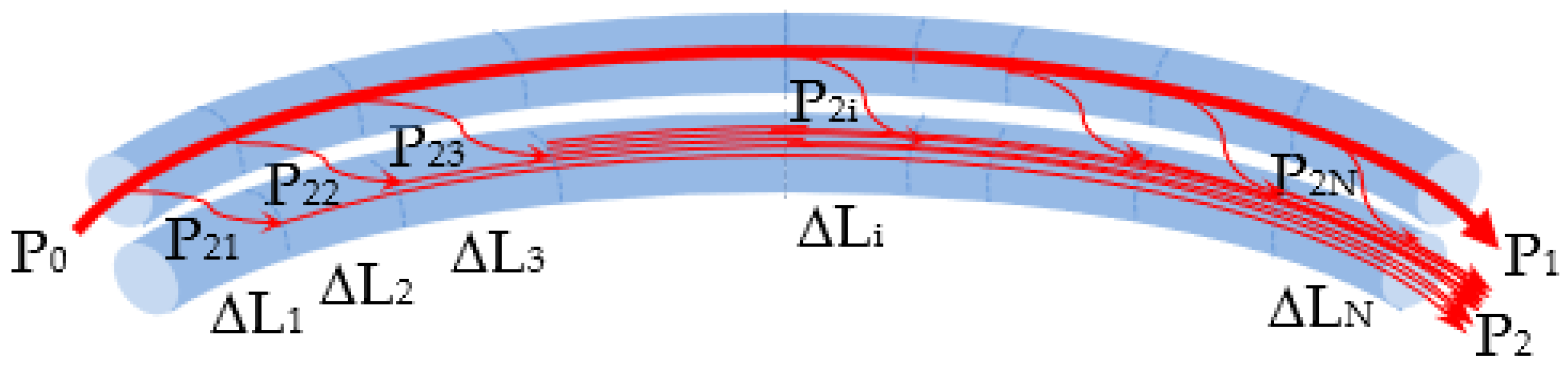
2. General Crosstalk Formulation Using CMT

The theoretical analysis follows the approach presented in Ref. [8] using the CMT. It is well known that for a uniform coupled two-core fiber without random perturbations, the power exchanges periodically between the two cores, which does not reflect experimental results of actual MCFs, in which measured crosstalk was much lower and accumulated linearly along the fiber length [10] due to random perturbations. Figure 1 shows a schematic of a two-core fiber with random perturbations, such as bending, twisting, and other index variations. Under random perturbations, the phases and polarizations of electrical fields in the two cores will change randomly along the fiber, and the coupled mode equations for a uniform fiber cannot be applied directly. To analyze the crosstalk under random perturbations, the fiber is divided into N uniform segments with lengths ΔL₁, ΔL₂, …, ΔL_N. To represent the random perturbation effects, we assume that the length of each segment is not necessarily the same, but can vary, and has a certain distribution, such as uniform, Gaussian, or exponential distribution. It is assumed that in each uniform segment, the electrical fields have constant phases and polarizations so that we can apply the CMT to each segment of the two cores. Optical power P₀ is launched into Core 1. In each uniform segment, a small amount of power is coupled to Core 2. For the two-core case, using the CMT, the amplitude A_m of the electric field E_m of the mode in core m within j-th uniform segment is described by the following coupled mode equations [15]:

$$\frac{d{A}_{mj}}{dz}=-i{\displaystyle \sum }_{n=1}^2{\kappa }_{mnj}{A}_{nj}\mathit{exp}\left(i\Delta {\beta }_{mnj}z\right) m=1, 2 ; j=1,2,\dots N$$

(1)

where m and n denote the core number, j is the segment number, κ_mnj is the mode coupling coefficient between the two cores, and Δβ_mnj is the difference in propagation constants of the two cores:

$$\Delta {\beta }_{mnj}={\beta }_{mj}-{\beta }_{nj}$$

(2a)

Noting that ${\kappa }_{11j}={\kappa }_{22j}=0$, $\mathsf{\Delta }{\beta }_{11j}=\mathsf{\Delta }{\beta }_{22j}=0$, to simplify the notations, we define ${\kappa }_j={\kappa }_{12j}={\kappa }_{21j}$, $\mathsf{\Delta }{\beta }_j={\beta }_{2j}-{\beta }_{1j}$. The difference in propagation constants $\Delta {\beta }_j$ is sensitive to external random perturbations. To consider the random perturbation effect, we write $\Delta {\beta }_j$ in the following form

$$\Delta {\beta }_j=\Delta {\beta }_0+\Delta {\beta }_{pj}$$

(2b)

which contains a constant term Δβ₀ due to the core designs without any external perturbations, and a term Δβ_pj due to random perturbations.

With the initial conditions of A₁₀ = A₀ and A₂₀ = 0 and the assumption of low crosstalk (A₁₁ = A₁₀), by solving the coupled mode equations, the amplitude of the electric field in Core 2 at the end of each uniform segment can be obtained [15]:

$$A_{2j}=i{A}_0{e}^{i\frac{1}{2}\Delta {\beta }_0\Delta L_j}{e}^{i\frac{1}{2}\Delta {\beta }_{pj}\Delta L_j}\frac{{\kappa }_j}{g_j}\sin \left(g_j\Delta L_j\right) j=1,2,\dots N$$

(3a)

and the electric field can be written as

$$E_{2j}=A_{2j}cos{\phi }_j\overrightarrow{x_0}+A_{2j}sin{\phi }_j\overrightarrow{y_0} j=1,2,\dots N$$

(3b)

where

$$g_j^2={\kappa }_j^2+{\left(\frac{\Delta {\beta }_j}{2}\right)}^2,$$

(4)

φ_j is the polarization angle with respect to the x-axis, and $\overrightarrow{x_0}$ and $\overrightarrow{y_0}$ are unit vectors in the x and y directions. The term Δβ_pj causes random phase changes in the field amplitude $A_{2j}\left(\Delta L_j\right)$. Furthermore, the polarization state is sensitive to external perturbations, which causes the polarization angle of the electric field to rotate randomly in each section. For simplicity, we assume that segment lengths represent distances beyond which the phase and polarization become uncorrelated due to random perturbations, and thus consider the segments to have an E-field with a random phase and polarization that are uniformly distributed in the [0, 2π] interval. The total power is calculated based on the vector electric field at the end of the fiber, $E={{\displaystyle \sum }}_{j=1}^N{E}_{2j}$ (see Appendix A for more details):

$$\begin{array}{c}{P}_2\left(L\right)=A_0^2{\displaystyle {\displaystyle \sum }_{j=1}^N}\left[{\left(\frac{{\kappa }_j}{g_j}\right)}^2{\sin }^2\left(g_j\Delta L_j\right)\right]\hfill \\ +A_0^2{\displaystyle {\displaystyle \sum }_{\begin{array}{c}j,k=1\hfill \\ j\ne k\hfill \end{array}}^N}\left[e^{i\frac{1}{2}\Delta {\beta }_0\left(\Delta L_j-\Delta L_k\right)}{e}^{i\frac{1}{2}\left(\Delta {\beta }_{pj}\Delta L_j-\Delta {\beta }_{pk}\Delta L_k\right)}\frac{{\kappa }_j{\kappa }_k}{g_j{g}_k}\sin \left(g_j\Delta L_j\right)\sin \left(g_k\Delta L_k\right)cos({\phi }_{jk})\right]\hfill \end{array}$$

(5)

where φ_jk is the angle between the electric field polarizations of segments j and k. In general, the uniform segment lengths for the phase and polarization may be different. For example, the polarization varies over longer segment lengths than the phase. In this case, the segment lengths are determined by the phase, and the polarization state can be treated unchanged over several segments in the simulation.

The crosstalk is given by $X=P_2/P_1$,

$$\begin{array}{c}X={\displaystyle {\displaystyle \sum }_{j=1}^N}\left[{\left(\frac{{\kappa }_j}{g_j}\right)}^{2}si{n}^2\left(g_j\Delta L_j\right)\right]\hfill \\ +{\displaystyle \sum }_{\begin{array}{c}j,k=1\\ j\ne k\end{array}}^N\left[e^{i\frac{1}{2}\Delta {\beta }_0\left(\Delta L_j-\Delta L_k\right)}{e}^{i\frac{1}{2}\left(\Delta {\beta }_{pj}\Delta L_j-\Delta {\beta }_{pk}\Delta L_k\right)}\left(\frac{{\kappa }_j}{g_j}\frac{{\kappa }_k}{g_k}\right)sin\left(g_j\Delta L_j\right)sin\left(g_k\Delta L_k\right)cos\left({\phi }_{jk}\right)\right]\hfill \end{array}$$

(6)

The above formulation is valid when the propagation constants do not change in each segment length ∆L. Therefore, it applies when the MCF is deployed with a constant bend radius R_b and a small twist rate α, such that ∆L ≪ l_α, where l_α = 2π/α is the twist period. This condition is satisfied when the correlation length is short and the fiber twist rate is low, which, in practice, is the case for most fiber deployments. If this condition is not met, i.e., ∆L > l_α, a numerical integration over each segment for the exponential term in Equation (1) can be used to obtain the amplitude $A_{2j}\left(\Delta L_j\right)$. In Section 4, we will illustrate an example of numerical integration for the exponential term when the twist period is short.

Equation (6) shows that, for a fiber with random perturbations, the crosstalk depends on the statistical distributions of the length, phase, and polarization of the uniform segments. As a result, the crosstalk also has a statistical distribution. Because the power is proportional to the square of the electric field, the crosstalk follows the χ²-square distribution as reported in earlier studies [6,16,17,18]. The crosstalk distribution depends on fiber uniformity due to manufacturing, deployment conditions, such as bends, twists, and thermal and mechanical stress effects. Thus, the fiber deployment condition will change the distribution and shift the average crosstalk value. For the purposes of transmission system engineering, the average crosstalk is an important parameter to determine the average system penalty, and the crosstalk distribution is used to provide an extra margin for a certain outage probability. Since the average power can be added incoherently, the average crosstalk value can be evaluated by the first simulation term only in Equation (6). The average crosstalk is related to the fiber segment distribution, the coupling coefficient, and the phase mismatch between the cores. Although the average crosstalk can be evaluated through numerical calculations of the first term of Equation (6), it would be more convenient to derive analytical expressions for the average crosstalk.

3. Analytical Expressions for Average Crosstalk

3.1. Derivation of Analytical Expressions

The average crosstalk is obtained by taking the average of Equation (6) over the random phase due to the random change in Δβ_j and Δβ_k and over the random polarization angle φ_jk. Because the phases and polarizations are correlated within each segment, and uncorrelated between segments, the second term of Equation (6) averages to zero. This can also be understood by examining the random phase changes due to Δβ_j and Δβ_k and the random polarization changes due to ${\phi }_{jk}$ in the second term of Equation (6). These random changes in phases and polarizations cause the crosstalk to have a distribution around an average value that is determined by the first term in Equation (6). Since the first term in Equation (6) does not depend on the polarization angle, the average crosstalk $\overline{X}$ is calculated over Δβ:

$$\begin{array}{c}\overline{X}=\langle {\displaystyle {\displaystyle \sum }_{j=1}^N}\left[{\left(\frac{{\kappa }_j}{g_j}\right)}^2{\sin }^2\left(g_j\Delta L_j\right)\right]{\rangle }_{\Delta \beta }=\frac{L}{L_c}\langle \frac{{{\displaystyle \sum }}_{j=1}^N\left[{\left(\frac{{\kappa }_j}{g_j}\right)}^2{\sin }^2\left(g_j\Delta L_j\right)\right]}{N}{\rangle }_{\Delta \beta }\hfill \\ =\frac{L}{L_c}\langle \langle {\left(\frac{\kappa }{g}\right)}^2{\sin }^2\left(g\Delta L\right){\rangle }_{\Delta L}{\rangle }_{\Delta \beta }\hfill \end{array}$$

(7)

where ${\langle f\rangle }_p$ denotes the average of a function f over a parameter p, L_c is the correlation length, which is assumed to correspond to the average segment length, and L = NL_c is the total fiber length. In the final form of Equation (7), the discrete average is replaced by the continuous function average, and κ_j and g_j are treated as continuous variables κ and g. To further simplify the derivation process and our numerical simulations, we assume that the coupling coefficient κ does not change along the fiber. Because the effect of coupling coefficient variation on crosstalk is expected to be much smaller than that due to the random phase changes in practical fibers, this simplification does not affect the main conclusions from our analyses.

We evaluate first the average crosstalk over the fiber segment length ΔL. To examine the effects of the segment length distribution on the average crosstalk, we consider the following three statistical distributions for the segment length ΔL:

$$f_s\left(\Delta L\right)=\left\{\begin{array}{ll}\delta \left(\Delta L-L_c\right)\hfill & \mathrm{Dirac}\hfill \\ \frac{1}{L_c}\exp \left(-\frac{\Delta L}{L_c}\right)\hfill & \mathrm{Exponential}\hfill \\ \frac{1}{\sqrt{2\pi }\sigma }\exp \left(-\frac{{\left(\Delta L-L_c\right)}^2}{2{\sigma }^2}\right)\hfill & \mathrm{Gaussian}\hfill \end{array}\right.$$

(8)

where σ is the standard distribution for Gaussian distribution. Note that Equation (8) is for the length segment distribution, which is different from the autocorrelation function in Refs. [7,10]. The average crosstalk for the three distributions becomes (See Appendix B):

$${\langle X\rangle }_{\Delta L}={\left(\frac{\kappa }{g}\right)}^2\frac{L}{L_c}{\sin }^2\left(g\Delta L\right)=\left\{\begin{array}{ll}\frac{{\kappa }^{2}L{\sin }^2\left(g{L}_c\right)}{g^2{L}_c}\hfill & \mathrm{Dirac}\hfill \\ \frac{2{\kappa }^{2}L{L}_c}{1+4g^2{L}_c^2}\hfill & \mathrm{Exponential}\hfill \\ \frac{{\kappa }^{2}L{L}_c\left[1-\cos \left(2g{L}_c\right)e^{-2{\sigma }^2{g}^2}\right]}{2g^2{L}_c^2}\hfill & \mathrm{Gaussian}\hfill \end{array}\right.$$

(9)

In the case of fiber deployment with bends, $g$ depends on the bending radius and twist angle, based on the definition in Equation (4) for $g$,

$$g^2={\kappa }^2+{\left(\frac{\Delta \beta }{2}\right)}^2$$

(10)

Figure 2 shows a two-core fiber under a bend. Using the equivalent index model of bent fiber [6], the propagation constants for the two cores and their difference are:

$${\beta }_1={\beta }_{0,1}\left(1+\frac{r_1}{R_b}\cos \left({\theta }_1\right)\right)$$

(11a)

$${\beta }_2={\beta }_1={\beta }_{0,1}\left(1+\frac{r_1}{R_b}\cos \left({\theta }_1\right)\right)$$

(11b)

$$\Delta \beta ={\beta }_2-{\beta }_1=\Delta {\beta }_0+\left({\beta }_{0,2}\frac{r_2}{R_b}\cos \left({\theta }_2\right)-{\beta }_{0,1}\frac{r_1}{R_b}\cos \left({\theta }_1\right)\right)$$

(11c)

where, $\Delta {\beta }_0={\beta }_{0,2}-{\beta }_{0,1}$, $\left(r_{1, } {\theta }_1\right)$ and $\left(r_2, {\theta }_2\right)$ are local coordinates of the centers of the two cores and $R_b$ is the bending radius. In general, $\Delta {\beta }_0$ is much smaller than ${\beta }_{0,1}$ and ${\beta }_{0,2}$, using the approximation ${\beta }_{0,1}\approx {\beta }_{0,2}\approx {\beta }_0$ we can write ${\beta }_{0,2}={\beta }_{0,1}+\Delta {\beta }_0\approx {\beta }_0+\Delta {\beta }_0$.

Using the relationship $r_2\cos \left({\theta }_2\right)-r_1\cos \left({\theta }_1\right)=Dcos\left(\theta \right)$ (see Figure 2), we can derive

$$\Delta \beta ={\beta }_0\frac{D}{R_b}\cos \left(\theta \right)+\Delta {\beta }_0+\Delta {\beta }_0\frac{r_2}{R_b}\cos \left({\theta }_2\right)$$

(12)

Here, $D$ is the distance between the cores. We see that the last term in the definition of $\Delta \beta$ is much smaller than the other terms, and we ignore this term in our subsequent calculation.

Since $\Delta \beta$ depends on the bending angle θ, the average of crosstalk over $\Delta \beta$ is evaluated over θ. In a deployment fiber, twisting is present and the bending angle changes with the fiber twist so that $\theta =\alpha z$, where $\alpha$ is the twist rate and $z$ is the distance along the fiber. The final average crosstalk is evaluated by taking the average of Equation (9) over a twist period,

$$\overline{X}={\langle \langle X\rangle }_{\Delta L}{\rangle }_{\theta }=\frac{1}{2\pi }{{\displaystyle \int }}_0^{2\mathsf{\pi }}{\langle X\rangle }_{\Delta L}d\theta =\frac{\alpha }{2\pi }{{\displaystyle \int }}_0^{2\pi /\alpha }{\langle X\rangle }_{\Delta L}dz$$

(13)

We see that the average crosstalk over a twist period is independent of the twist rate $\alpha$. To simplify the notations, we define the following parameters

$$a=\kappa L_c,\hspace{1em}b=\frac{{\beta }_{0}D}{2R_b}{L}_c,\hspace{1em}c=\frac{\Delta {\beta }_0}{2}{L}_c$$

(14)

where a, b, and c represent the phase changes due to mode coupling, fiber bending, and core mismatch between the two cores. We can change Equation (13) to

$$\overline{X}={\kappa }^{2}L{L}_{c}f\left(a,b,c\right)$$

(15)

where

$$f\left(a,b,c\right)=\frac{1}{2\pi }{{\displaystyle \int }}_0^{2\pi }h\left(a,b,c\right)d\theta$$

(16)

The integrand function $h\left(a,b,c\right)$ has the following form

$$h\left(a,b,c\right)=\left\{\begin{array}{ll}\frac{{\sin }^2\left(G\right)}{G^2}\hfill & \mathrm{Dirac}\hfill \\ \frac{2}{1+4G^2}\hfill & \mathrm{Exponential}\hfill \\ \frac{1-\cos \left(2G\right)\exp \left(-2{\mathsf{\Sigma }}^2{G}^2\right)}{2G^2}\hfill & \mathrm{Gaussian}\hfill \end{array}\right.$$

(17)

where

$$G^2=a^2+{\left(b\cos \left(\theta \right)+c\right)}^2$$

(18)

G is the total phase factor due to mode coupling, fiber bending, and core mismatch between the two cores. Here, the standard deviation $\Sigma =\sigma /L_c$ is normalized to the unit of the correlation length $L_c$.

Equation (17) shows how the crosstalk changes for the three distributions of $\Delta L$ for the case when the fiber is straight without bending, corresponding to the formulas described in Ref. [8]. From Equation (17), we can see that for the Dirac distribution, the crosstalk oscillates with $G$ following a sinc function. For the exponential distribution, the crosstalk is the moving average over an oscillation period of the sinc function for the Dirac distribution. Furthermore, we can see that the crosstalk in the Dirac distribution and the exponential distribution are the limits of the crosstalk of the Gaussian distribution depending on $\Sigma$ and G. When $\Sigma G\gg 1$, the crosstalk of Gaussian distribution is close to that of exponential distribution. When $\Sigma G\ll 1$, the crosstalk of Gaussian distribution is close to that of Dirac distribution. Figure 3 plots the function h versus the parameter G for the three distributions. For the Gaussian distribution, we plot two curves with $\Sigma =0.1\mathrm{and}2$, respectively. It can be seen clearly that function h in the exponential distribution is the average of the Dirac distribution. Furthermore, for the Gaussian distribution, when $\Sigma =2$, the h is very close to that for exponential distribution. When $\Sigma =0.1$ and $G<13$, the function h is similar to that for the Dirac function, exhibiting oscillations. When $\Sigma =0.1$ and $G>13$, the function h is similar to that for the exponential function.

For the exponential distribution, we will show that we can obtain an analytical formula for the average crosstalk as a function of the bending angle. For the other two distributions, we will analyze the asymptotic behavior and show that the average crosstalk is very close to that of the exponential distribution. Therefore, we can apply the analytical formula derived from the exponential distribution as a general formula for calculating the average crosstalk.

For the exponential distribution, the function $f\left(a,b,c\right)$ is given by

$$f\left(a,b,c\right)=\frac{2}{\pi }{{\displaystyle \int }}_0^{\pi }\frac{d\theta }{A^2+{\left(B\cos \left(\theta \right)+C\right)}^2}$$

(19)

where

$$A^2=1+4a^2,\hspace{1em}\hspace{1em}B=2b,\hspace{1em}\hspace{1em}C=2c$$

(20)

The integral can be computed as the ratio of the sum of the square roots of the complex number and its conjugate to its magnitude times a constant factor

$${{\displaystyle \int }}_0^{\pi }\frac{d\theta }{A^2+{\left(B\cos \left(\theta \right)+C\right)}^2}=\frac{\pi }{2}\frac{\sqrt{Z}+\sqrt{\overline{Z}}}{A\left|Z\right|}$$

(21)

where $Z$ is a complex number defined as

$$Z=A^2+B^2-C^2+2iAC$$

(22)

Using the formula for the square root of a complex number (see Appendix C), the function $f\left(a,b,c\right)$ takes the following form:

$$f\left(a,b,c\right)=\frac{\sqrt{2}\sqrt{\left|Z\right|+\mathrm{Re}\left(Z\right)}}{A\left|Z\right|}$$

(23)

The average crosstalk for the case of exponential distribution can be computed analytically using Equations (14), (15), (20), and (23). We can show that Equation (15) is equivalent to Equation (16) in Ref. [11] if the parameter $a=\kappa L_c$ in the parameter G is equivalent to null (see Appendix D). Therefore, our analytical expressions are more general than analytical expressions in Ref. [11]. Because the parameter a is generally very small, both analytical expressions are expected to give the same results. However, for a homogeneous MCF without bending, b = 0 and c = 0, our analytical expression is still valid and reduced to the same expression Equation (9) in Ref. [8] for exponential distribution.

Next, we show that we can derive simpler formulas from the analytical equations under certain conditions, which allow us to understand better the crosstalk variation. For the homogeneous case $c=0$, the Formula (23) simplifies to:

$$f\left(a,b,0\right)=\frac{2}{A\sqrt{A^2+B^2}}$$

(24)

By substituting A and B into Equation (24), and assuming $a\ll 1$, which is satisfied by weakly coupled MCF, we get a general crosstalk formula for the homogeneous MCF,

$$\overline{X}=\frac{2{\kappa }^{2}L{L}_c}{\sqrt{1+{\left(\frac{{\beta }_{0}D}{R_b}{L}_c\right)}^2}}$$

(25)

which is equal to Equation (23) in Ref. [11]. Equation (25) shows that the crosstalk for homogeneous MCF depends on both the bending radius and the correlation length. If $b\gg 1$, the average crosstalk from Equation (25) becomes

$$\overline{X}=2{\kappa }^2\frac{R_{b}L}{{\beta }_{0}D}$$

(26)

matching the formula from Hayashi et al. [6]. This formula is valid for a bend radius $R_b\ll {\beta }_{0}D{L}_c$. In this case, the crosstalk is determined by the bending radius only, as shown in Equation (26). For a large bending radius when $R_b\gg {\beta }_{0}D{L}_c$, the crosstalk is determined by the correlation length only, the same as Equation (20) in Ref. [11], as shown below:

$$\overline{X}=2{\kappa }^{2}L{L}_c$$

(27)

Figure 4 plots the crosstalk as a function of R_b using Equation (25) for various L_c. The parameters used in Figure 4 are:

$$\begin{array}{ll}\lambda \hfill & =1550 \mathrm{nm},\hspace{1em}{n}_{eff}=1.447,\hfill \\ \kappa \hfill & =0.007532 {\mathrm{m}}^{-1},\hspace{1em}L=2 \mathrm{m},\hspace{1em}D=45 \mathsf{\mu }\mathrm{m}\hfill \end{array}$$

where n_eff is the effective refractive index of the mode in each core. The crosstalk calculated using Equation (26) corresponds to the curve of $L_c=\infty$, which is a not a realistic case. For shorter L_c, the approximation of Equation (26) is good only for small R_b, around tenths of millimeters. For large R_b, the crosstalk is determined by the correlation length as in Equation (27).

For heterogeneous MCF, for the case of a≪1, b≫1 and $\left|c\right|\ll b$, we can simplify Equation (23) and derive

$$\overline{X}=2{\kappa }^2\frac{R_{b}L}{{\beta }_{0}D}$$

(28)

which is the same as Equation (27) in Ref. [19]. Equation (28) is identical to Equation (26) for the homogeneous core design. This result indicates that when the bending-induced phase mismatch dominates, the crosstalk is proportional to the bend radius for both the homogeneous and heterogeneous MCF. For heterogeneous MCF, the Formula (28) is valid for bend radii smaller than a critical value R_c. By setting $\left|b\right|\approx \left|c\right|$, we can get the same critical bend radius expression as derived in Ref. [11]

$$R_c=\frac{{\beta }_0}{\Delta {\beta }_0}D$$

(29)

Equation (29) shows that the critical radius R_c is inversely proportional to the phase Δβ₀ mismatch between the two cores. For a bending radius much less than the critical bending radius R_c, the crosstalk is determined by the bending radius, as shown in Equation (28). For a bending radius much larger than the critical bending radius R_c, or $\left|b\right|\ll \left|c\right|$ and $\left|c\right|\gg a$, the crosstalk becomes [11]:

$$\overline{X}=2\frac{{\kappa }^2}{\Delta {\beta }_0^2}\frac{L}{L_c}$$

(30)

In this case, the crosstalk is inversely proportional to the correlation length and the phase mismatch squared.

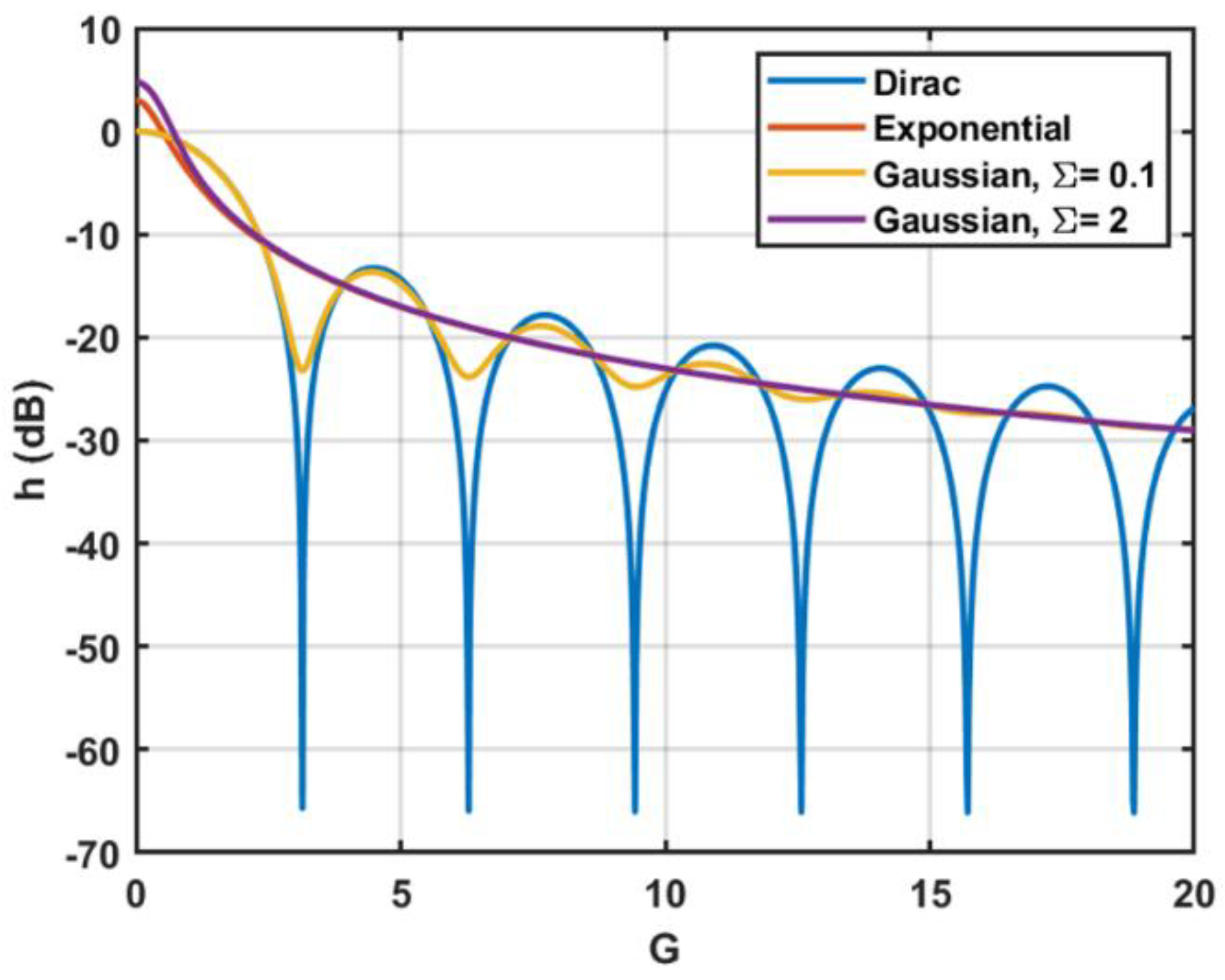
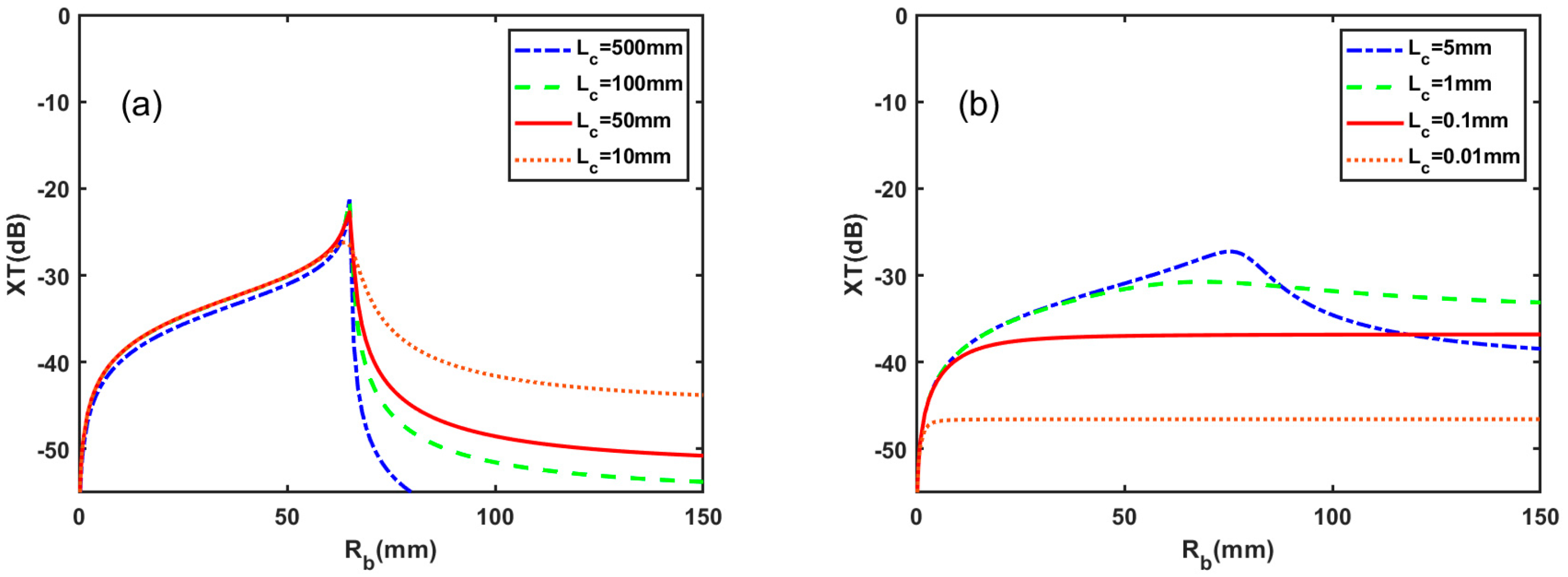
3.2. Comparison of Average Crosstalk for Different Statistical Distributions

In the following, we compare the average crosstalk for the three distributions. For the exponential distribution, the crosstalk is calculated using the analytical expression for function f in Equation (23). For the Dirac and Gaussian distributions, the function f is evaluated via numerical integration of Equation (16). We compute the average crosstalk for all three distributions and correlation lengths $L_c=0.005,0.5 \mathrm{m}$. The standard deviation for the Gaussian distribution is set to $\sigma =L_c$. We use the following parameters in our calculations:

$$\begin{array}{ll}\lambda \hfill & =1550 \mathrm{nm},\hspace{1em}{n}_{eff}=1.44,\hspace{1em}\Delta n_{eff}=0.046\%,\hfill \\ \kappa \hfill & =0.742 {\mathrm{m}}^{-1},\hspace{1em}L=2 \mathrm{m},\hspace{1em}D=30 \mathsf{\mu }\mathrm{m}\hfill \end{array}$$

where $\Delta n_{eff}$ is the effective refractive index difference between the two cores, which can be used to determine the phase mismatch $\Delta {\beta }_0$ between the two cores.

Figure 5 shows the average crosstalk for the two correlation lengths. We see that the average crosstalk for the exponential distribution is very close to the other two distributions for a wide range of bending radii and two correlation lengths, $L_c$. The critical radius R_c, calculated using Equation (29), is 65 mm, corresponding to the peak crosstalk. Again, the crosstalk of the exponential distribution is the average of the Dirac distribution. For the Gaussian distribution, the crosstalk is very close to the exponential distribution. The results show that the analytical formula that uses Equation (23) derived from the exponential distribution is a very good approximation of the average crosstalk for the Dirac and Gaussian distributions. Therefore, the statistical distribution inside a fiber segment length does not influence that much the average crosstalk, and we can employ the analytical formula for the average crosstalk in all three statistical distribution cases.

3.3. Comparison with the Results in the Literature for the Heterogeneous Case

In this section, we compare our analytical formulas of Equations (17) and (25) with the results that were reported in Ref. [11]. We use the same parameters as in in Section 3.2 to compute the crosstalk for the correlation lengths L_c = 500, 100, 50, 10, 5, 0.5, 0.05, 0.01 mm.

Our results for the above parameters are shown in Figure 6, which agree with the results from Figure 5 reported by Koshiba et al. [11]. The critical bending radius is calculated using Equation (29), which is 65 mm. The results of using the analytical formula support the statement that our analytical expressions are equivalent to Ref. [11], as shown in Appendix D.

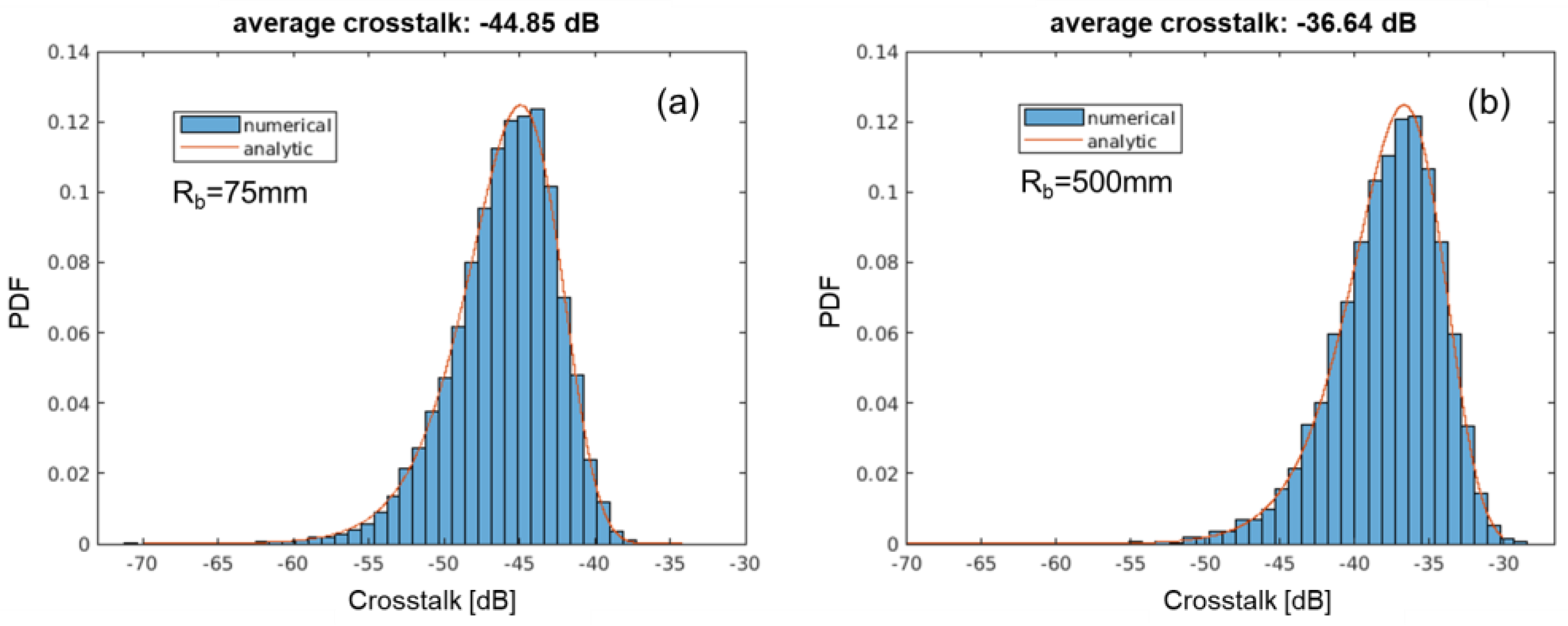
4. Numerical Simulations and Comparisons with Analytical Expressions

Equation (6) for the crosstalk lends itself to a numerical evaluation based on statistical distributions of random perturbations. For a given MCF core design, geometry, length, and deployment condition, we generate 10⁴ random realizations of the fiber (sufficient to achieve converged numerical results), in which phase and polarization perturbations occur between fiber uniform segments ∆L_j and ∆L_j+1, with lengths distributed according to a correlation-scale dependent function. In the following simulations we use statistical distributions of ∆L defined in Equation (8), to implement correlation-scale dependent function. Figure 7 shows crosstalk distributions evaluated for a 1 km long two-core homogeneous MCF with core spacing D = 45 µm, coupling coefficient κ = 0.007532 m⁻¹, Gaussian distribution with L_c = 0.04 m, and λ = 1.55 µm. The numerical model is based on Equation (5) for the total coupled power, which is computed based on the simulation of vector E-field contributions, given by Equation (3b), from each segment to the total E-field in the coupled core. Therefore, the simulated crosstalk accounts for both components of the E-field polarization. The numerical results for bend radii of 75 mm and 500 mm, representative of deployment on a shipping spool and in a fiber cable, are compared with analytic solutions [6] given by a χ²-distribution function with four degrees of freedom, indicating good agreement between the two approaches.

The dependence of average crosstalk on the bend radius is shown in Figure 8a for the same MCF parameters as in Figure 7, comparing results from numerical simulation with those predicted by numerical evaluation of Equations (15) and (16), as well as analytic expressions for R_b⁻¹ = 0 from [8] and for R_b⁻¹ > 0 from [11]. In the case of Gaussian distribution function f_s(∆L), numerical results match well the straight fiber crosstalk value predicted by the expression specified in [8]. Good agreement between all methods is also seen for bend radii extending to R_b ≈ 5 m, matching in this range the estimate based on analytic formula in [6] for average crosstalk at small bend radii. Numerical simulations for the case of exponential distribution of segment lengths are found to be in full correspondence with the analytic result from Equation (12) of [11] for all bend radii. In the case of Dirac distribution ∆L = L_c, the crosstalk obtained from Equation (15) closely matches the corresponding result from numerical simulations, including the asymptotic value at R_b⁻¹ = 0. Similar to the average crosstalk, at small bend radii there is also a good agreement between the corresponding probability density functions simulated assuming different statistical distributions of ∆L (Figure 8b), as concluded also in Section 3.2, which are modeled well by a χ²-distribution function.

The impact of correlation length parameter L_c on the average crosstalk is shown in Figure 9 for the case of straight deployment of MCF with the same parameters as discussed above, and for the case with a larger mode coupling coefficient (κ = 0.012 m⁻¹), representing a change of core design. Numerical results from statistical simulations and from analytic expression in [8] are found to be in very good agreement.

Crosstalk distributions for heterogenous core MCF with the same parameters as in Figure 7, but a difference of ∆n_eff = 5 × 10⁻⁴ in the effective refractive index of the modes of two cores, are shown in Figure 10. The average crosstalk for large bend radii deployment, R_b = 500 mm, is reduced significantly compared to homogeneous MCF, while for R_b = 75 mm, the stronger coupling due to tighter bends leads to a smaller difference between heterogenous and homogeneous core configurations. In both cases, the numerically computed crosstalk distributions are approximated well by a χ²-distribution fit to simulation data.

A comparison of the average crosstalk computed from numerical simulations and predicted by Equations (15) and (16) for heterogenous MCF is shown in Figure 11. For bend radii R_b < 1 m, the average crosstalk and probability density function are practically independent of the distribution function assumed for ΔL, and for all bend radii the analytic solutions are confirmed by the numerical simulations. The average crosstalk in the R_b⁻¹ = 0 limit also does not depend significantly on the assumption of either exponential or Gaussian distribution functions; however, it can differ significantly for the case of constant ∆L, due to oscillatory dependence of the crosstalk on the bend radius.

As we discussed earlier in Section 2, Equation (1) is derived assuming that the difference in propagation constants of the cores is constant over the segment length ∆L. Therefore, it applies when the MCF is deployed with a constant bend radius R_b and a small twist rate α, such that ∆L ≪ l_α, where l_α = 2π/α is the twist period. To evaluate the accuracy of this approximation we consider MCF parameters and deployment conditions for the case “Perfectly homogeneous MCF” presented in Figure 1 of Ref. [13]. The dashed line in Figure 12 is evaluated using numerical simulations based on the Equation (3a) assuming averaging over the twist period, as described in the manuscript. It is seen to be in good agreement with the corresponding result labeled “dashed line: estimate by expression proposed in [18]” as presented in Figure 1 of Ref. [13]. We verified the solution in this regime by numerically integrating Equation (1) over each segment length ∆L with an integration step size much less than ∆L and R_b. The result is shown by the open red symbols that coincide with the dashed line (only a few points common to both cases are shown for clarity).

In the case when the twist period is comparable to the segment length, or the correlation length, the more general form of Equation (1) with the accumulated phase (e.g., as described by Equation (1a,b) in Ref. [13]) should be used. The approach presented in the manuscript can be applied in this case by replacing the crosstalk amplitude given by Equation (3a) at the end of the segment of length ∆L, by the amplitude found by the integration of the more general form of Equation (1) with the accumulated phase. We evaluated this approach by numerically integrating Equation (1) modified to include the accumulated phase that includes the variation due to the twist. The result is shown in Figure 12 by red solid circles, which reproduce the corresponding oscillatory curve shown by a solid line (and square symbols) in Figure 1 of Ref. [13].

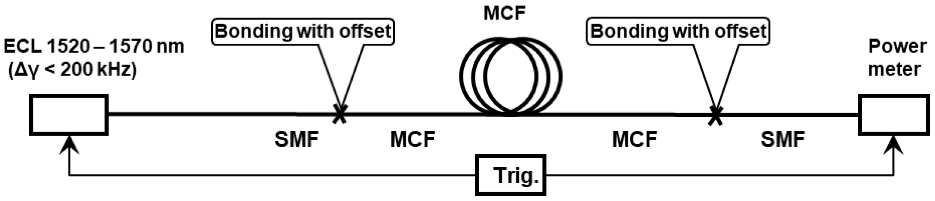
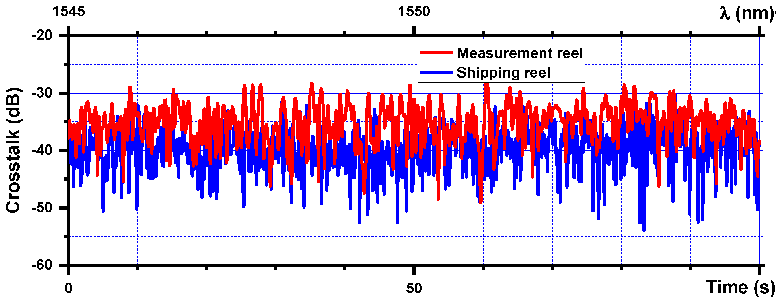
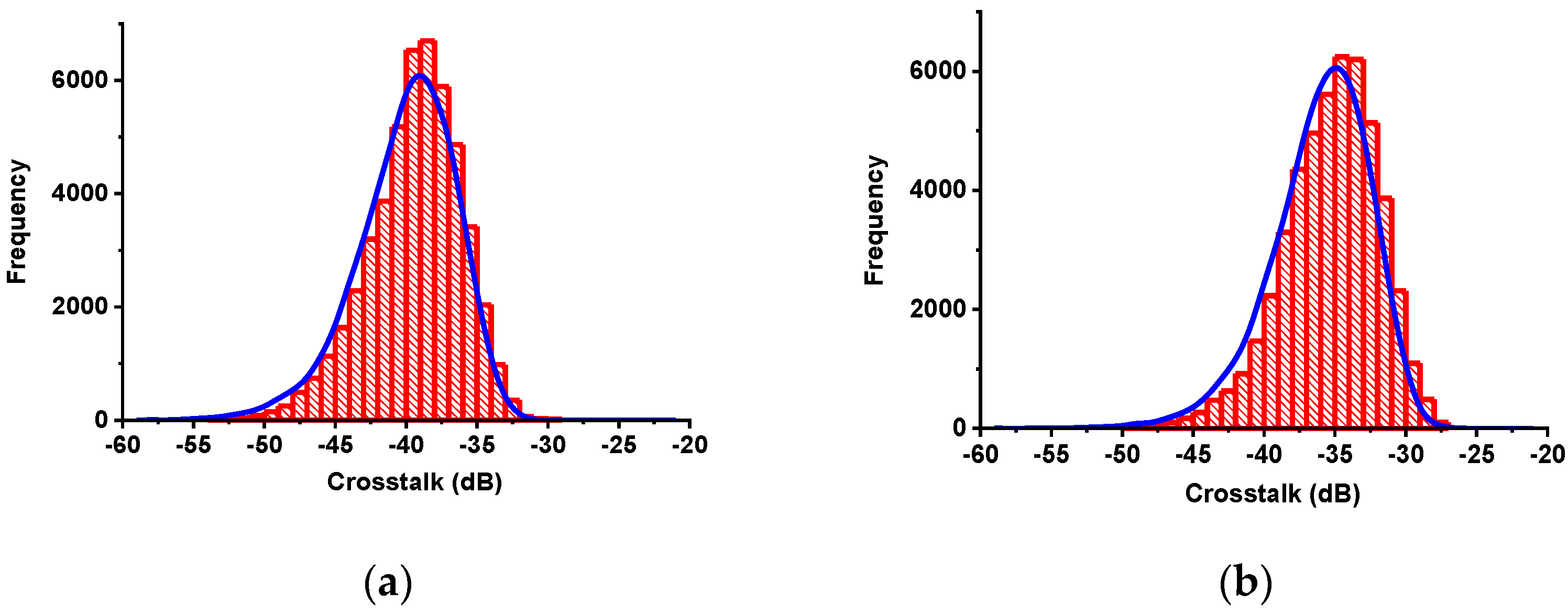
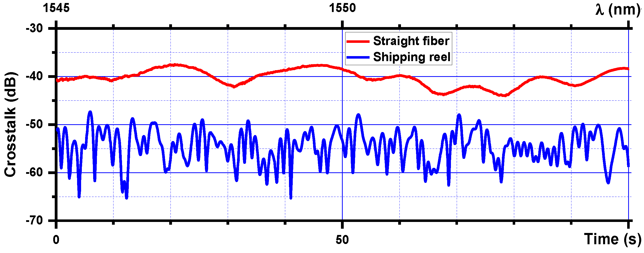
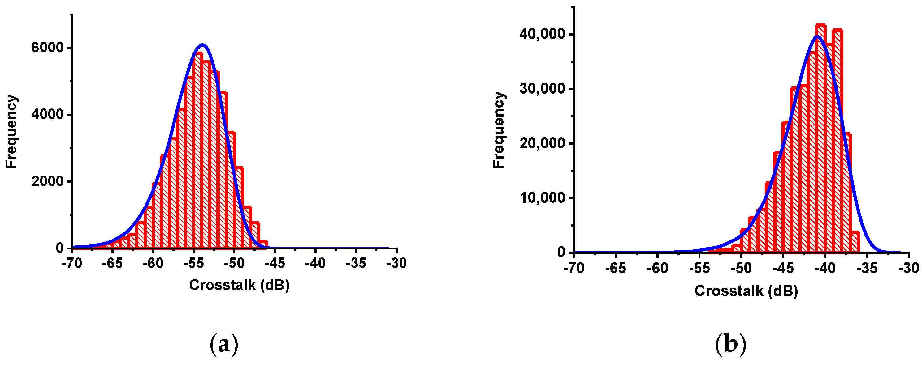
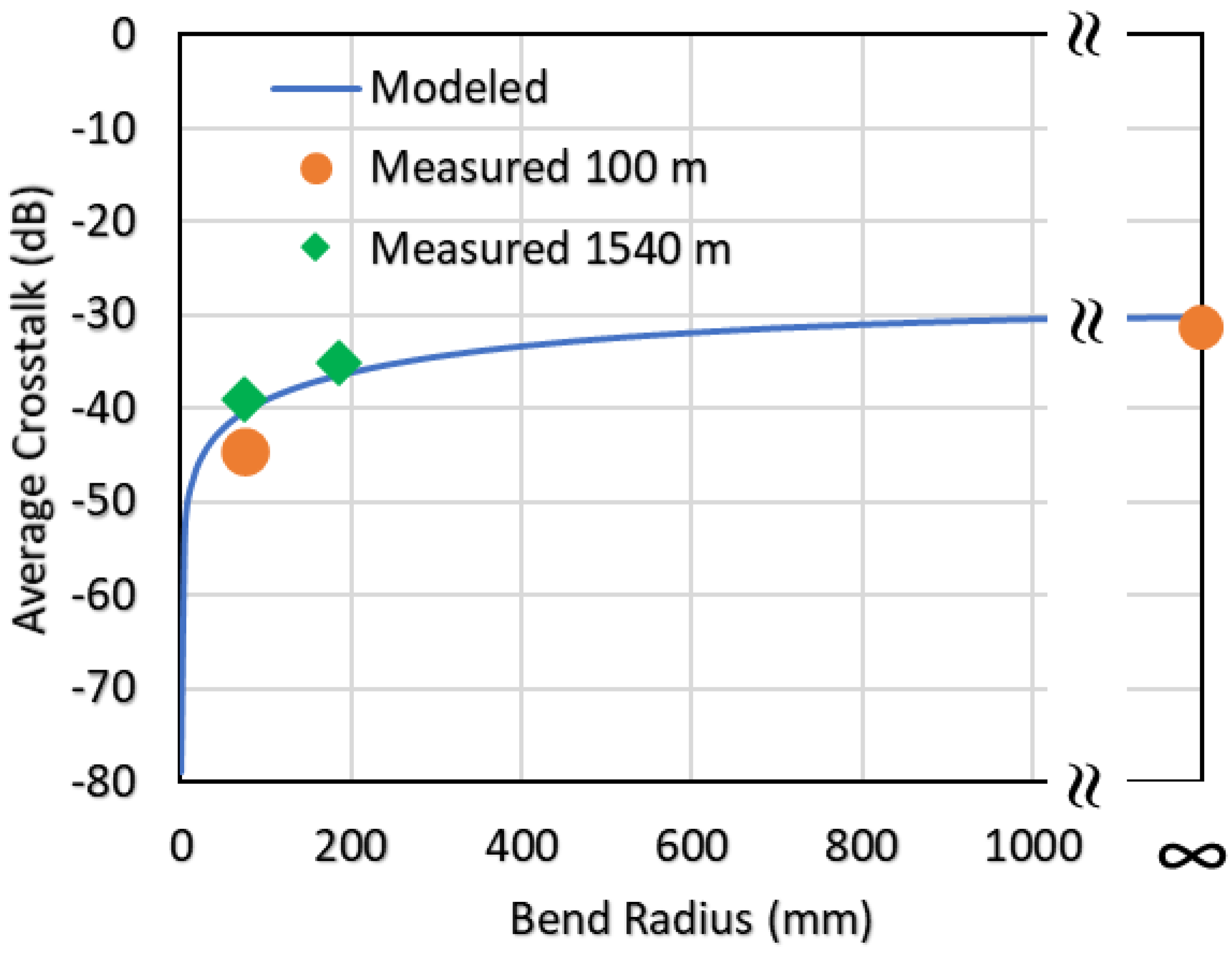
5. Experimental Characterization of MCF Crosstalk Statistical Distributions

Experimental characterization of crosstalk has been reported in various papers, see e.g., [9,16,18,20]. In Ref. [16], a method was developed to measure the extremely low crosstalk of MCF statistically. In Ref. [19], the statistical behavior of the inter-core crosstalk power in weakly coupled MCFs with multiple interfering cores was experimentally assessed. In Ref. [9], it was shown that a crosstalk statistical distribution can be characterized with different types of perturbations, such as thermal, mechanical, or wavelength scanning, to yield the same result. In current research we use the wavelength scanning technique to compare crosstalk for MCF deployed under three different bending conditions: a shipping reel with radius of 75 mm, a measurement reel with radius of 185 mm, and a straight line.

Figure 13 shows a schematic of the experimental setup. An external cavity laser, tunable in the range of 1520–1570 nm, is used as light source. The MCF used in our experiments is a two-core fiber with a homogeneous core design. The core refractive index profile is similar to the standard single-mode fiber (SMF) design. Each core is Germanium doped with a step relative refractive index of 0.34%, and a core diameter of 8.5 μm. The core spacing is about 44 μm. The cladding is pure silica with a diameter of 125 μm (Figure 14a). The coupling coefficient is estimated to be 0.01052 1/m, calculated from the fiber design. Although the fiber is designed as a homogeneous two-core fiber, fluctuations can happen in fiber manufacturing to cause the two cores to be slightly different, which leads to slightly different parameters in the two cores. We estimated the mismatch in Δβ₀ and found that the value was much smaller than the coupling coefficient κ, which means that the parameter $c=\Delta {\beta }_0/2·L_c$ can be ignored in our model. Therefore, the fiber can be considered as a homogeneous fiber in our theoretical analysis to compare with experimental data. The light is coupled into one core of MCF through a 2 m standard SMF bonded by UV-curing adhesive with lateral offset (Figure 14b). The light output from another core of the MCF is sent to the power meter through another 2 m standard SMF bonded with lateral offset. Crosstalk power variation in time is detected by a power meter with a 10 ms sampling interval, while continuous mode-hop-free linear scanning of the laser wavelength within 10 or 50 nm interval is performed.

We first measured crosstalk with 1540 m of fiber wound on shipping and measurement reels and compared the crosstalk distributions and the average crosstalk. We then measured the crosstalk of fiber under a straight deployment condition, where the fiber has two straight ~50 m sections with a ~1 m radius U-turn in the middle. Due to the space limitation, we used only 100 m for this measurement. The fiber was attached in several locations to the floor by scotch tape along the walls of a 50 m corridor. To compare with the fiber under a bending condition, we also measured the same 100 m fiber wound on a shipping reel. The measurement results allow us to analyze crosstalk scaling with both the bending radius and the fiber length.

In the case of 1540 m length of MCF wound on shipping and measurement reels, we found fast variations of crosstalk power over time during laser wavelength scanning within 10 nm intervals, as shown in Figure 15, that correspond to instantaneous crosstalk variations, as observed in previous papers (see e.g., [16,21]). Furthermore, we observed an increase of the average crosstalk for the larger diameter measurement reel.

Figure 16 shows statistical distributions of crosstalk (50,000 aggregate sampling points for five different scans) for the 1540 m long fiber in both dB and linear scales. Compared with the results for the fiber on the shipping reel, the measurement reel deployment increases the average crosstalk by about 4.2 dB, but the distributions are very similar following a χ²-distribution that was obtained from numerical simulations of the same number of samples as in the experiment. In the model we used an exponential distribution of segment lengths with L_c = 0.006 m, and a coupling coefficient that was 15% larger than the theoretical coupling coefficient from the fiber design to obtain the best match to the measured data. To quantify how well the modeled curves fit to the experimental data, we evaluated the fitting quality parameter, delta, which is the absolute difference between simulated and measured crosstalk distributions, by computing the sum of absolute values of the differences in frequency counts of the two discrete distributions of linear crosstalk, normalized by the total number of samples. For the 1540 m long MCF sample deployed on the shipping and measurement reels, the delta was computed to be 0.13 and 0.16, respectively. We also computed the difference between the average crosstalk evaluated from the model and experimental data. The absolute difference was found to be 0.6 dB and 0.3 dB for the shipping and measurement reels, respectively.

For the 100-m-long fiber deployed on the shipping reel and under the straight condition, crosstalk power variations in similar scans are shown in Figure 17. We found that for the fiber on the shipping reel, the power evolution over time was much slower than for the longer fiber length as compared with Figure 15. A crosstalk statistical distribution could be obtained from a single scan with 10,000 sampling points, but the distribution function was not very smooth and there was about a 1.5 dB variation for the average crosstalk in different scans. Thus, we repeated scans five times to get 50,000 aggregate sampling points and squeezed fiber on a reel by palms between scans to get better randomization of the data. For the straight fiber deployment, the average crosstalk was much higher and power evolution over time was even much slower (see Figure 17). In this case, it was very difficult to obtain a smooth crosstalk distribution even using repetitive scans. Thus, we performed scans for several days and used 10 nm and 50 nm scan intervals (entire number of sampling points is 320,000). The origin of a slower evolution of crosstalk over time (wavelength) for a shorter fiber span and straight deployment condition is not clear so far, but we hypothesize that it might be resulted from reduced perturbations due to fewer overlapping fiber layers on the fiber reel, or less bending and twisting in the straight deportment condition. The reduced perturbations to fiber could decrease random variations in phases and polarization states with time, which result in a slower evolution of crosstalk.

Figure 18 shows the statistical distributions of crosstalk for the fiber of 100 m length measured on the shipping reel and in the straight-line condition. Again, both distributions follow a χ²-distribution (blue line at Figure 18). At the same time, sharp decay for high crosstalk levels at Figure 18b may be conditioned by poor randomization of crosstalk states, especially for 10 nm scan intervals. In Figure 18 for 100 m MCF, the same model parameters were used to generate the simulation results as in Figure 16 for a 1540-m-long sample, but with a coupling coefficient that was 20% smaller than a coupling coefficient from the fiber design for a better match to the measured distributions. The variations in the coupling coefficient used for fitting may be indicative of its length dependence due to fiber parameter variations of the MCF parameters in practice. For a 20% fluctuation in the coupling coefficient, the average crosstalk changes by about less than 1.9 dB, which is small compared to the average crosstalk magnitude. We also calculated the fitting quality parameter delta for the 100-m-long MCF sample on the shipping reel and straight deployment, the delta was found to be 0.14 and 0.17, respectively. The absolute difference in average crosstalk was found to be 0.6 dB and 1.1 dB for the shipping reel and the straight condition, respectively.

The normalized difference in frequency counts between simulated and measured crosstalk distributions is between 0.13 and 0.17 for both 100 m and 1540 m MCF samples, and for all deployment conditions considered in the experiment. While this metric does not distinguish between differences near the average and tails of the statistical distributions, the relatively small (≤17%) difference and narrow range of variation of delta with deployment conditions, as well as ≤1.1 dB difference in average crosstalk values, indicates an overall level of agreement that makes the model useful for transmission system engineering applications.

The average measured crosstalk in the straight deployment condition is −41.8 dB, an increase of about 13 dB in comparison with the shipping reel (−54.5 dB). Compared with the measurement result of 1540 m fiber on the shipping reel, we get −51.3 dB for 100 m using the linear length scaling rule. The measured average crosstalk results can be compared with the computed average crosstalk using Equation (26). To perform the comparison, we normalized the measured average crosstalk with different fiber lengths to 1 km using the linear scaling rule. Using the coupling coefficient calculated from the fiber design and the correlation length of 0.006 m used in the crosstalk distribution simulation, we obtain the average crosstalk dependence on the bend radius shown in Figure 19. The four measured crosstalk data points for bend radii of 75 mm, 185 mm, and infinity agree well with the crosstalk calculated from Equation (26).

6. Discussions

In this paper, a simple numerical simulation method is presented on crosstalk using the CMT by treating an MCF as concatenated uncorrelated segments with a random segment length distribution. This method is different from other approaches that have been considered previously, such as the discrete changes model of crosstalk [21], and its generalization to dual-polarization cases (DP-DCM) [22], which are derived based on the crosstalk evaluated at discrete phase matching points These formulations have the advantage of being computationally efficient, and, in the case of DP-DCM, also suitable for modeling coherent and direct-detection MCF transmission systems. The current derivation, on the other hand, is based on the direct integration of coupled mode amplitude equations in each MCF segment with constant properties, requiring ~10⁴ random fiber realizations for numerical evaluation of crosstalk distribution, which is less than 10⁷ that may be required by other methods [18].

This new simulation method allows us to derive a general closed-form simulation formula Equation (6) for the crosstalk of MCFs under random perturbations, which contains a term for the average crosstalk and a term for the crosstalk distribution. It is a simple formula that is easy to use for simulating crosstalk numerically. In addition, it provides physical insight about crosstalk behaviors. The first term does not depend on the random phase and random polarization changes, which represents the average crosstalk. If one is interested in the average crosstalk only, only the simple expression of the first terms needs to be used to provide quick results. The second term depends on random phase and polarization changes, which represents the statistical distribution of crosstalk. This term can be used for fast numerical simulations of the statistical nature of crosstalk.

As we pointed out in Section 2, the closed-form simulation formula is valid for an MCF deployed under a constant bend radius R_b and a small twist rate α, or a long twist period l_α, such that ∆L ≪ l_α. This condition is satisfied in many practical fiber deployments. For example, when the fiber is wound on a shipping spool of 150 mm diameter, a typical condition for fiber measurements, the natural twist period is over 100 m. For the fiber inside a cable, the twist period is a much longer 1 m for fiber reliability reasons. Therefore, the condition of ∆L ≪ l_α is met by most practical applications.

We further study the crosstalk under three different statistical distribution of the segment lengths. We show that the statistical distribution of segment length changes the detailed average crosstalk behavior but does not affect the overall crosstalk trend. For the exponential distribution of segment length, we derive a simple analytical expression for the average crosstalk, which can be used for system engineering applications. Our analytical expression is more general than that in Ref. [11], and agrees with the results of Ref. [11] when parameter $a=\kappa L_c$ is small compared to the parameters of b and c.

We provide detailed numerical simulations using the general closed-form simulation formula and compare these with results from various analyses. The numerical simulation results provide validation of our general closed-form simulation formula and show that it can be applied to fibers with various perturbations.

We also measure crosstalk under two different bending conditions and a straight condition. To the best of our knowledge, the crosstalk under the straight condition has not been reported so far. The measured crosstalk distributions and average crosstalk provide further validation to our modeling results.

In our analytical and numerical modeling, we assume that the coupling coefficient does not vary along the fiber for simplicity. This assumption is supported by our experimental data. The measurement results of the average crosstalk of different sections of the fiber indicate 15% to 20% variations in the coupling coefficient. For a 20% fluctuation in the coupling coefficient, the average crosstalk change is only about 1.9 dB, which is much smaller compared to the average crosstalk magnitude of −30 dB or lower for weakly coupled MCFs. Therefore, the assumption of constant coupling coefficient is a good approximation for practical MCFs.

The model presented in this paper can be expanded for future studies. The two-core model can be generalized to more interfering cores to evaluate their contributions to the total crosstalk to one core. Furthermore, we can apply the model to practical cable structures with certain twisting and bending diameters to study the effects of cabling on crosstalk. In this paper, we analyze only the properties of crosstalk of MCF with a CW laser at its input. For transmission systems, it is more interesting to evaluate the effects of crosstalk on signal performance in coherent or direct-detection systems, as well as the impact of instantaneous crosstalk on the outage probability of an optical communication system. The extension of our crosstalk model to transmission systems will also be a subject for future study.

7. Conclusions

We have presented a study of MCF crosstalk using the CMT. We derived a general closed-form simulation formula for the crosstalk of MCF under random perturbations. This general formulation allows evaluations of both the average crosstalk and the crosstalk statistical distribution. We analyzed the average crosstalk under three statistical distributions of fiber uniform segment lengths, constant, exponential, and Gaussian, and derived simple analytical expressions for the average crosstalk. We also performed numerical simulations for crosstalk statistical distributions using the general closed-form simulation formula and showed that crosstalk distributions agree well with the χ²-distribution function with four degrees of freedom. Furthermore, the average crosstalk from numerical simulations agrees with the approximation from the simple analytical expressions. Finally, we conducted crosstalk measurements under different bending deployment conditions. The results show that the measured crosstalk distributions and the average crosstalk agree with our modeling results.

References

1. Nakajima, K.; Sillard, P.; Richardson, D.; Li, M.; Essiambre, R.; Matsuo, S. Transmission media for an SDM-based optical communication system. IEEE Commun. Mag. 2015, 53, 44–51. [Google Scholar] [CrossRef]
2. Li, M.J.; Hayashi, T. Chapter 1—Advances in Low-Loss, Large-Area, and Multicore Fibers; Willner, A.E., Ed.; Optical Fiber Telecommunications VII; Academic Press: Cambridge, MA, USA, 2020; pp. 3–50. ISBN 9780128165027. [Google Scholar] [CrossRef]
3. Kunimasa, S.; Shoichiro, M. Multicore fibers for large capacity transmission. Nanophotonics 2013, 2, 441–454. [Google Scholar] [CrossRef]
4. Butler, D.L.; Li, M.-J.; Li, S.; Geng, Y.; Khrapko, R.R.; Modavis, R.A.; Nazarov, V.N.; Koklyushkin, A.V. Space Division Multiplexing in Short Reach Optical Interconnects. J. Light. Technol. 2017, 35, 677–682. [Google Scholar] [CrossRef]
5. Fini, J.M.; Zhu, B.; Taunay, T.F.; Yan, M.F. Statistics of crosstalk in bent multicore fibers. Opt. Express 2010, 18, 15122–15129. [Google Scholar] [CrossRef] [PubMed]
6. Hayashi, T.; Taru, T.; Shimakawa, O.; Sasaki, T.; Sasaoka, E. Design and fabrication of ultra-low crosstalk and low-loss multi-core fiber. Opt. Express 2011, 19, 16576–16592. [Google Scholar] [CrossRef] [PubMed]
7. Koshiba, M.; Saitoh, K.; Takenaga, K.; Matsuo, S. Multi-core fiber design and analysis: Coupled-mode theory and coupled-power theory. Opt. Express 2011, 19, B102–B111. [Google Scholar] [CrossRef] [PubMed]
8. Li, M.; Li, S.; Modavis, R.A. Coupled Mode Analysis of Crosstalk in Multicore Fiber with Random Perturbations. In Proceedings of the 2015 Optical Fiber Communications Conference and Exhibition (OFC), Los Angeles, CA, USA, 22–26 March 2015; pp. 1–3. [Google Scholar]
9. Nazarov, V.; Kuchinsky, S.A.; Zakharian, A.R.; Li, M.J. Crosstalk Statistical Distributions in Multicore Fibers Under Different Deployment Conditions. In Proceedings of the 2021 Optical Fiber Communications Conference and Exhibition (OFC), Washington, DC, USA, 6–10 June 2021. [Google Scholar]
10. Takenaga, K.; Arakawa, Y.; Tanigawa, S.; Guan, N.; Matsuo, S.; Saitoh, K.; Koshiba, M. An investigation on crosstalk in multi-core fibers by introducing random fluctuation along longitudinal direction. IEICE Trans. Commun. 2011, E94-B, 409–416. [Google Scholar] [CrossRef]
11. Koshiba, M.; Saitoh, K.; Takenaga, K.; Matsuo, S. Analytical Expression of Average Power-Coupling Coefficients for Estimating Intercore Crosstalk in Multicore Fibers. IEEE Photonics J. 2012, 4, 1987–1995. [Google Scholar] [CrossRef]
12. Antonelli, C.; Riccardi, G.; Hayashi, T.; Mecozzi, A. Role of polarization-mode coupling in the crosstalk between cores of weakly coupled multi-core fibers. Opt. Exp. 2020, 28, 12847–12861. [Google Scholar] [CrossRef] [PubMed]
13. Cartaxo, A.V.P.; Morgado, J.A.T. New Expression for Evaluating the Mean Crosstalk Power in Weakly-Coupled Multi-Core Fibers. J. Light. Technol. 2021, 39, 1830–1842. [Google Scholar] [CrossRef]
14. Wang, W.; Xiang, L.; Shao, W.; Shen, G. Stochastic Crosstalk Analyses for Real Weakly Coupled Multicore Fibers Using a Universal Semi-Analytical Model. J. Light. Technol. 2021, 39, 4503–4510. [Google Scholar] [CrossRef]
15. Marcuse, D. Theory of Dielectric Optical Waveguides, 2nd ed.; Academic Press: Cambridge, MA, USA, 1991. [Google Scholar]
16. Hayashi, T.; Taru, T.; Shimakawa, O.; Sasaki, T.; Sasaoka, E. Characterization of Crosstalk in Ultra-Low-Crosstalk Multi-Core Fiber. J. Light. Technol. 2012, 30, 583–589. [Google Scholar] [CrossRef]
17. Gan, L.; Shen, L.; Tang, M.; Xing, C.; Li, Y.; Ke, C.; Tong, W.; Li, B.; Fu, S.; Liu, D. Investigation of channel model for weakly coupled multicore fiber. Opt. Express 2018, 26, 5182–5199. [Google Scholar] [CrossRef] [PubMed]
18. Alves, T.; Soeiro, R.; Cartaxo, A. Probability Distribution of Intercore Crosstalk in Weakly Coupled MCFs With Multiple Interferers. IEEE Photonics Technol. Lett. 2019, 31, 651–654. [Google Scholar] [CrossRef]
19. Hayashi, T.; Sasaki, T.; Sasaoka, E.; Saitoh, K.; Koshiba, M. Physical interpretation of intercore crosstalk in multicore fiber: Effects of macrobend, structure fluctuation, and microbend. Opt. Express 2013, 21, 5401–5412. [Google Scholar] [CrossRef] [PubMed]
20. Alves, T.M.F.; Cartaxo, A.V.T.; Rebola, J.L. Stochastic Properties and Outage in Crosstalk-Impaired OOK-DD Weakly-Coupled MCF Applications with Low and High Skew × Bit-Rate. IEEE J. Sel. Top. Quantum Electron. 2020, 26, 4300208. [Google Scholar] [CrossRef]
21. Cartaxo, A.V.T.; Alves, T.F.M. Discrete changes model of inter-core crosstalk of real homogeneous multi-core fibers. J. Light. Technol. 2017, 35, 2398–2408. [Google Scholar] [CrossRef]
22. Soeiro, R.O.J.; Alves, T.M.F.; Cartaxo, A.V.T. Dual Polarization Discrete Changes Model of Inter-Core Crosstalk in Multi-Core Fibers. IEEE Photonics Technol. Lett. 2017, 29, 15. [Google Scholar] [CrossRef] [Green Version]
Figure 1. Schematic of mode coupling in a two-core fiber that is divided into N uncorrelated uniform segments.
Photonics 10 00174 g001
Figure 2. Schematics of a two-core fiber under a bend with a radius Rb and the local coordinates used in the equivalent index model.
Photonics 10 00174 g002
Figure 3. The h function vs. the parameter G for three distributions.
Photonics 10 00174 g003
Figure 4. Crosstalk vs. the bending radius R for Equation (25) for various L c and Equation (26).
Photonics 10 00174 g004
Figure 5. Average crosstalk dependence on the bend radius for correlation length Lc= 0.005 m (a) and Lc = 0.5 m (b).
Photonics 10 00174 g005
Figure 6. (a) Crosstalk as a function of bending radius, for correlation length, 500 mm, 100 mm, 50 mm, and 10 mm; (b) crosstalk as a function of bending radius, for correlation length, 5 mm, 1 mm, 0.1 mm, and 0.01 mm.
Photonics 10 00174 g006
Figure 7. Probability density functions of two-core homogeneous MCF, computed numerically (histograms) and analytically [6] (line) for deployments with bend radii (a) Rb = 75 mm and (b) 500 mm.
Photonics 10 00174 g007
Figure 8. (a) Average crosstalk dependence on the bend radius, computed numerically and based on analytic approaches of M. Koshiba et al. 2012 [11], M. Li et al. 2015 [8] and Equation (15); (b) simulated crosstalk probability density functions for homogeneous MCF at Rb = 500 mm in comparison to the χ2-distribution function.
Photonics 10 00174 g008
Figure 9. Average crosstalk dependence on the correlation length scale Lc, computed numerically and based on analytic expression from [8] for the case of (a) Gaussian and (b) exponential distribution of uniform segment lengths.
Photonics 10 00174 g009
Figure 10. Probability density functions of two-core heterogenous MCF (neff = 5 × 10⁻⁴), computed numerically for deployments with bend radii (a) Rb = 75 mm and (b) 500 mm. Dashed lines show the fit of χ2-distribution function with four degrees of freedom to numerical data.
Photonics 10 00174 g010
Figure 11. (a) Average crosstalk dependence on the bend radius computed analytically according to M. Koshiba et al. 2012 [11], M. Li et al. 2015 [8], numerically and based on Equation (15), for heterogeneous cores with ∆neff = 5 × 10⁻⁴; (b) simulated crosstalk probability density functions for heterogeneous MCF at Rb = 500 mm in comparison to the χ2-distribution function.
Photonics 10 00174 g011
Figure 12. Average crosstalk for “ideal homogeneous” MCF parameters from Figure 1 of [13]. Dashed line: computed via numerical simulations based on Equation (3a) assuming averaging over the twist period. Open red circles: computed numerically by integrating Equation (1) over each segment length ∆L with an integration step ∆z much smaller than ∆L and Rb, and assuming averaging over the twist period. Filled red circles: computed numerically by integrating Equation (1) modified to include the accumulated phase ∆θ(z) that includes the variation due to the twist with period of 0.134 m.
Photonics 10 00174 g012
Figure 13. Measurement setup for crosstalk statistical characterization.
Photonics 10 00174 g013
Figure 14. Images of cleaved end face of two-core MCF (a) and bonded with lateral offset standard single-mode and MCF (b).
Photonics 10 00174 g014
Figure 15. Crosstalk variations with laser wavelength scanning for the fiber of 1540 m length on shipping and measurement reels.
Photonics 10 00174 g015
Figure 16. Crosstalk statistical distribution functions for 1540 m long fiber: (a) shipping reel; (b) measurement reel. Blue lines: modeled χ2-distributions.
Photonics 10 00174 g016
Figure 17. Crosstalk variations with laser wavelength scanning for straight and reeled fiber of a 100 m length.
Photonics 10 00174 g017
Figure 18. Crosstalk statistical distribution functions for 100 m fiber: (a) shipping reel; (b) straight fiber. Blue lines: modeled χ2-distributions.
Photonics 10 00174 g018
Figure 19. Comparison of measured and modeled crosstalk as a function of bend radius.
Photonics 10 00174 g019
Disclaimer/Publisher’s Note: The statements, opinions and data contained in all publications are solely those of the individual author(s) and contributor(s) and not of MDPI and/or the editor(s). MDPI and/or the editor(s) disclaim responsibility for any injury to people or property resulting from any ideas, methods, instructions or products referred to in the content.