On the Fluctuations of Internal DLA on the Sierpinski Gasket Graph

Abstract

Internal diffusion limited aggregation (IDLA) is a random aggregation model on a graph G, whose clusters are formed by random walks started in the origin (some fixed vertex) and stopped upon visiting a previously unvisited site. On the Sierpinski gasket graph, the asymptotic shape is known to be a ball in the graph metric. In this paper, we improve the sublinear bounds for the fluctuations known from its known asymptotic shape result by establishing bounds for the odometer function for a divisible sandpile model.

1. Introduction

The internal diffusion limited aggregation model (IDLA), which was introduced by Diaconis and Fulton in [1], is a stochastic aggregation model grown by consecutively started particles, where a particle is added upon exiting the current cluster. Let G be an infinite but locally finite connected graph with a specified vertex ∘ acting as the origin of these particles. Let ${\left(X^1\left(t\right)\right)}_{t\ge 0},{\left(X^2\left(t\right)\right)}_{t\ge 0},\dots$ be a sequence of independent simple random walks on G started in ∘, representing the particles. The IDLA cluster $\mathcal{I}\left(i\right)$ after $i\ge 0$ particles is now iteratively defined as

$$\begin{array}{cc}\hfill & \mathcal{I}\left(0\right)=\varnothing ,\mathcal{I}\left(i\right)=\mathcal{I}(i-1)\cup \left\{X^i\left({\sigma }^i\right)\right\}\hfill \end{array}$$

where ${\sigma }^i=inf\{t\ge 0|X^i\left(t\right)\notin \mathcal{I}(i-1)\}$ is the first time that particle i leaves the existing cluster. So, the first particle stops immediately at ∘ and $\mathcal{I}\left(1\right)=\{\circ \}$. After i particles, the cluster contains exactly i vertices, i.e., $\left|\mathcal{I}\right(i\left)\right|=i$. Notice that ${\left(\mathcal{I}\left(i\right)\right)}_{i\ge 0}$ is a Markov chain on the connected subsets of G. An important question concerning IDLA is the typical shape of the random set $\mathcal{I}\left(i\right)$ for large i. On ${\mathbb{Z}}^d$, Lawler, Bramson and Griffeath [2] identified the limit shape as a Euclidean ball, and later in [3], Lawler improved the bounds for the fluctuations. Finally, later in [4,5], these bounds were further improved to sublogarithmic bounds for $d\ge 3$ and logarithmic ones for $d=2$ in [6,7] via two different approaches. Convergence to a scaling limit, that is, rescaling the graph of ${\mathbb{Z}}^d$ and taking the limit of clusters started from a particle distribution rather than a single source, is shown in [8] for IDLA and two other aggregation models. For finitely generated groups having exponential growth in [9], the authors prove a shape theorem with a suitable metric. For the special case of homogeneous trees, the authors also give lower bounds for the fluctuations from this basic shape. In [10], the author proves an inner bound for IDLA on supercritical percolation clusters, whereas in [11], a corresponding outer bound (depending on the inner bound) is established. For the comb, i.e., ${\mathbb{Z}}^2$ without all horizontal edges except the x-axis, [12] show a basic shape result and in [13], fluctuations are established. On the cylinder graph, that is, ${\mathbb{Z}}_N\times \mathbb{Z}$, where ${\mathbb{Z}}_N$ is the cyclic group with N elements, a basic shape result, the fluctuations, and the existence of a coupling between two IDLA chains are introduced in [14]. See also [15] for a survey on IDLA and its counterpart: external DLA, where random walks start from outside the cluster.

Recently, some interest has developed in the study of aggregation models on fractals, namely on the double-sided Sierpinski gasket graph $SG$, which is defined as follows. Let

$$\begin{array}{cc}\hfill & V_0:=\left\{\left(0,0\right),\left(1,0\right),\left(1/2,\sqrt{3}/2\right)\right\},\hfill \\ \hfill & E_0:=\left\{\left(\left(0,0\right),\left(1,0\right)\right),\left(\left(1,0\right),\left(1/2,\sqrt{3}/2\right)\right),\left(\left(0,0\right),\left(1/2,\sqrt{3}/2\right)\right)\right\}\hfill \end{array}$$

and then recursively

$$\begin{array}{cc}\hfill V_{n+1}& =V_n\cup \left(\left(2^n,0\right)+V_n\right)\cup \left(\left(2^{n-1},2^{n-1}\sqrt{3}\right)+V_n\right),\hfill \\ \hfill E_{n+1}& =E_n\cup \left(\left(2^n,0\right)+E_n\right)\cup \left(\left(2^{n-1},2^{n-1}\sqrt{3}\right)+E_n\right),\hfill \end{array}$$

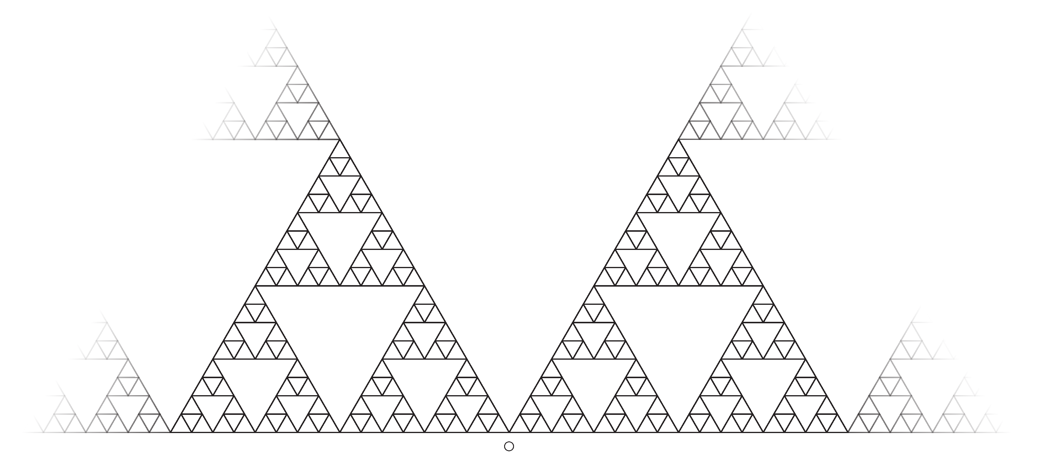
where $(x,y)+S=\left\{\right(x,y)+z|z\in S\}$. The Sierpinski gasket graph is defined by $(V_{\infty }={\bigcup }_{n\in \mathbb{N}}{V}_n,E_{\infty }={\bigcup }_{n\in \mathbb{N}}{E}_n)$ and from this, we obtain the double-sided Sierpinski gasket graph $SG$ by adding a copy of the one-sided version reflected along the y-axis, namely, $SG=(-V_{\infty }\cup V_{\infty },-E_{\infty }\cup E_{\infty })$. See Figure 1 for an illustration of $SG$.

Set $\circ =(0,0)$ as the origin, from which random walks are launched successively. We denote by $B_x\left(n\right)$ the closed graph metric balls of radius n centered at vertex x, and by $b_n:=\left|B_{\circ }\left(n\right)\right|$ the cardinality of the ball $B_{\circ }\left(n\right)$. In [16], Chen, Huss, Sava-Huss and Teplyaev prove a basic shape result on $SG$.

Theorem 1

(Theorem 1.1 of [16]). On $SG$, the IDLA cluster after $b_n=\left|B_{\circ }\left(n\right)\right|$ particles occupies a set of sites close to ball of radius n. That is, for all $\epsilon >0$ and n large enough, we have

$$\begin{array}{c}\hfill B_{\circ }\left(n(1-\epsilon )\right)\subseteq \mathcal{I}\left(b_n\right)\subseteq B_{\circ }\left(n(1+\epsilon )\right)\mathit{with}\mathit{probability}1.\end{array}$$

For the rotor router aggregation, which is a deterministic counterpart of IDLA starting rotor router walks instead of simple random walks, the shape of the cluster is exactly known to be a ball up to the fluctuations of $\pm 1$ from the radius [17]. In [18], the authors determine the shape of the divisible sandpile model, also a ball with respect to the graph metric. This yields that the universal shape conjecture—all three aggregation clusters share the same limit shape—holds true for $SG$. Furthermore, $SG$ is the only known non-trivial graph (other than $\mathbb{Z}$), where even a fourth model, the Abelian sandpile model, also shares this basic shape [17].

The Sierpinski gasket graph is originated as an approximation of the Sierpinski gasket, where the latter is a well-known nested fractal of Hausdorff dimension $\alpha =ln\left(3\right)/ln\left(2\right)$. In [19], the authors define a Brownian motion on the fractal as a limit of rescaled simple random walks on the Sierpinski gasket graph. The finite generation of the Sierpinski gasket graph can also be used to define a Dirichlet form and a Laplacian on the fractal; see the standard monographs [20,21] for an introduction to the analysis on the Sierpinski gasket. In [22], the author uses the Sierpinski gasket graph to define and study the spectral properties of the Laplacian on the infinite Sierpinski gasket. Additionally, the Sierpinski gasket graph itself found interest in research. From a probabilistic standpoint, the various properties of the random walk on $SG$ [23,24,25], the loop erased random walk [26,27], and the uniform spanning tree [27] have all been well studied. Combinatorial results, such as the average distances of vertices [28] and the number of spanning trees [27,29,30], have been established. An extension of the Sierpinski gasket to higher dimensions has also been studied in multiple aspects. In [31], the author calculates the exact measures of the gasket in any dimension $d\ge 2$. For dimension $d=3$ in [32], the authors investigate the loop erased random walk on the corresponding approximating graph and its continuum-limit process on the gasket. Again, on the graph, approximately for the three- and two-dimensional gasket, there exist geometric criteria to decide whether the shortest path between two vertices in neighboring triangles uses the common vertex of those triangles; see [33].

In this work, we will use the ideas from [3] to improve the sublinear fluctuations bounds of the IDLA cluster known from the basic shape Theorem 1.

Theorem 2.

On $SG$, the IDLA cluster after $b_n=\left|B_{\circ }\left(n\right)\right|$ particles satisfies, with probability 1 for any $\kappa >0$, some constant $c>0$ and n that is large enough:

$$\begin{array}{c}\hfill B_{\circ }\left(n-c{n}^{1/2}ln{\left(n\right)}^{(1+\kappa )/2\alpha }\right)\subseteq \mathcal{I}\left(b_n\right)\subseteq B_{\circ }\left(n+c{n}^{1/2+1/2\alpha }ln{\left(n\right)}^{(1-1/\alpha )(1+\kappa )/2\alpha }\right),\end{array}$$

where $\alpha =ln\left(3\right)/ln\left(2\right)$ is the Hausdorff dimension of the Sierpinski gasket.

The main improvement from the existing result is based on the analysis of the aforementioned divisible sandpile model, which was first introduced in [34]. In contrast to the Abelian sandpile model, it distributes non-integer mass to its neighbors during the toppling procedure, making it more tractable. We develop lower bounds for the odometer function for vertices with a certain distance to the boundary of the cluster in Section 3. We then use these bounds to prove the inner fluctuation of Theorem 2 in Section 4. The bounds for the outer bound in Section 5 work analogously to [11,16].

2. Preliminaries

Let $G=(V,E)$ be an infinite locally finite connected graph. For convenience, we write $x\in G$ instead of $x\in V$ and $x\sim y$ if $(x,y)\in E$. Furthermore, we write $d(x,y)$ for the usual graph distance between vertices $x,y\in G$, and for $x\in G$ and $A\subseteq G$, denote

$$\begin{array}{cc}\hfill deg\left(x\right)& :=\{z\in G|x\sim z\}\mathrm{the}\mathrm{vertex}\mathrm{degree}\mathrm{of}x,\hfill \\ \hfill B_x\left(n\right)& :=\{z\in G|d(x,z)\le n\}\mathrm{the}\mathrm{ball}\mathrm{of}\mathrm{radius}n\mathrm{with}\mathrm{center}x,\hfill \\ \hfill {\partial }_{I}A& :=\{y\in A|{\exists }_{z\notin A}y\sim z\}\mathrm{the}\mathrm{inner}\mathrm{boundary}\mathrm{of}A.\hfill \end{array}$$

Let ${\mathbb{P}}_x$ be the probability law of the simple random walk $X={\left(X\left(t\right)\right)}_{t\ge 0}$ on G started in vertex $x\in G$, and let ${\mathbb{E}}_x$ be the expectation with respect to ${\mathbb{P}}_x$. For this simple random walk, we define the stopping times

$$\begin{array}{ccc}\hfill & {\tau }_x\left(n\right):=inf\{t\ge 0|X\left(t\right)\in {\partial }_I{B}_x\left(n\right)\cup B_x^c\left(n\right)\},\hfill & \hfill \tau \left(n\right):={\tau }_{\circ }\left(n\right)\end{array}$$

and the stopped Green function

$$\begin{array}{c}\hfill g_n(x,y):={\mathbb{E}}_x\left(\sum _{n=0}^{\tau \left(n\right)-1}{\mathbb{1}}_{\left\{X\right(t)=y\}}\right),\end{array}$$

which plays a major role in the analysis of bounds of IDLA. For any function $f:G\to \mathbb{R}$, we define the (probabilistic) graph Laplacian as

$$\begin{array}{c}\hfill \Delta f\left(x\right):=\frac{1}{deg\left(x\right)}\sum _{y\sim x}h\left(y\right)-h\left(x\right)\end{array}$$

and call any $h:G\to \mathbb{R}$ satisfying $\Delta h\left(x\right)=0{\forall }_{x\in S}$ a harmonic function on $S\subseteq G$. It is easy to show that the aforementioned stopped Green function satisfies $\Delta g_n(\circ ,x)={\delta }_{\circ }\left(x\right)$ for all $x\in B_{\circ }\left(n\right)\setminus {\partial }_I{B}_{\circ }\left(n\right)$ and, therefore, is harmonic on $B_{\circ }\left(n\right)\setminus (\{\circ \}\cup {\partial }_I{B}_{\circ }\left(n\right))$.

Now, due to its special structure, one can derive three major properties of $SG$, all of which can be proven using coverings of proper triangles.

Lemma 1.

The $SG$ satisfies the following properties:

(EHI) 

The elliptic Harnack inequality: there exists a positive constant C such that for all $x\in G$, $n>0$, and functions $h\ge 0$ that are harmonic on $B_x\left(2n\right)$, the following holds:

$$\begin{array}{c}\hfill \underset{y\in B_x\left(n\right)}{sup}h\left(y\right)\le C\underset{y\in B_x\left(n\right)}{inf}h\left(y\right).\end{array}$$

$\left(V_{\alpha }\right)$

The uniform volume growth condition: there exist constants $c,C>0$ such that for all $x\in G$, $n>0$, the following holds:

$$\begin{array}{c}\hfill c{n}^{\alpha }\le \left|B_x\left(n\right)\right|\le C{n}^{\alpha }.\end{array}$$

$\left(E_{\beta }\right)$

The uniform exit time growth condition: there exist constants $c,C>0$ such that for all $x\in G$, $n>0$, the following holds:

$$\begin{array}{c}\hfill c{n}^{\beta }\le {\mathbb{E}}_x\left({\tau }_x\left(n\right)\right)\le C{n}^{\beta }.\end{array}$$

The respective constants in the exponents are $\alpha :=ln\left(3\right)/ln\left(2\right)$, the Hausdorff dimension, and $\beta :=ln\left(5\right)/ln\left(2\right)$, the walk dimension of the Sierpinski gasket.

Proof. 

See Chapter 2.2 of [35] for the proofs of $\left(V_{\alpha }\right)$ and $\left(E_{\beta }\right)$. The proof of $\left(EHI\right)$ is then given in Theorem 2.6 of [35]. □

For our proof of the inner bound in Theorem 2, we need some slightly sharper bounds than the ones used in Lemma 2.8, 2.10 of [16]. In fact, the proofs of such lemmas can be easily improved to obtain the following.

Lemma 2.

There exist constants $c_1,c_2>0$ such that for every $x\in SG$ and $n>0$, we have

$$\begin{array}{cc}\hfill {\mathbb{E}}_x\left({\tau }_{\circ }\left(n\right)\right)& \ge c_{1}d{(x,{\partial }_I{B}_{\circ }\left(n\right))}^{\beta }\mathit{and}\hfill \\ \hfill g_n(x,x)& \le c_{2}d{(x,{\partial }_I{B}_{\circ }\left(n\right))}^{\beta -\alpha }.\hfill \end{array}$$

In the following sections, occurring constants will always be denoted as $c\in \mathbb{R}$ and may differ from line to line.

3. The Divisible Sandpile

In this section, we will establish a lower bound in Lemma 7 needed for our arguments in Section 4. We derive this from the results in [18], which are briefly outlined here.

We call a function $\mu :SG\to [0,\infty )$ with finite support $\left|\mathrm{supp}\right(\mu \left)\right|<\infty$ a sand distribution, and we call any $x\in SG$ unstable if $\mu \left(x\right)>1$. Any unstable vertex can be toppled such that the excess mass $\mu \left(x\right)-1$ is split evenly among its neighboring vertices. The resulting distribution is then given by

$$\begin{array}{c}\hfill T_x\mu :=\mu +max\{\mu \left(x\right)-1,0\}\Delta {\delta }_x,\end{array}$$

where ${\delta }_x\left(y\right)$ equals 1 if $x=y$ and 0 otherwise. We call $T_x$ the toppling operator at vertex x. Note that there is no need for x to be an unstable vertex since, otherwise, $T_x=\mathrm{Id}$. We start with an initial sand distribution ${\mu }_0$, and let ${\left(x_k\right)}_{k\ge 1}$ be a sequence of vertices containing each vertex of $SG$ infinitely often. We call such sequences toppling sequences and define the sand distribution after k topples as

$$\begin{array}{c}\hfill {\mu }_k\left(y\right):=T_{x_k}{\mu }_{k-1}\left(y\right)=T_{x_k}\dots T_{x_1}{\mu }_0\left(y\right)\end{array}$$

as well as the odometer function $u_k$, which counts the mass emitted by a vertex up to k topples

$$\begin{array}{c}\hfill u_k\left(y\right):=\sum _{j\in \{i\le k|x_i=y\}}{\mu }_j\left(y\right)-{\mu }_{j+1}\left(y\right)=\sum _{j\in \{i\le k|x_i=y\}}max\{{\mu }_j\left(y\right)-1,0\}.\end{array}$$

Intuitively, toppling many vertices should spread the mass out such that the mass is covered by more and more vertices until there is not enough mass left to cover any new vertices. This intuition turns out to be the case as the next lemma states. Note here that [34] is dedicated to the case of ${\mathbb{Z}}^d$, but the proof works for any graph.

Lemma 3

(Lemma 3.1 of [34]). As $k\to \infty$, ${\mu }_k$ converges to a sandpile distribution μ and $u_k$ converges from below to a limit function u. Moreover, these limits satisfy

$$\begin{array}{c}\hfill \mu \left(z\right)={\mu }_0\left(z\right)+\Delta u\left(z\right)\mathit{and}\mu \left(z\right)\le 1,\mathit{for}\mathit{any}z\in SG.\end{array}$$

(1)

The least action principle Lemma 3.2 of [8] states that the odometer function u in Lemma 3 is the smallest function satisfying Equation (1). At first sight, the limits u and $\mu$ seem to depend on the choice of the toppling sequence selected for the toppling procedure. This, however, turns out not to be the case as the Abelian property of the divisible sandpile model states.

Lemma 4

(Lemma 3.6 of [18]). The limiting odometer function u is independent of the choice of the toppling sequence.

Therefore, we call $\mu$ the sand distribution and u the odometer function according to the starting distribution ${\mu }_0$; its sandpile cluster is defined as $\mathcal{S}:=\{z\in SG|\mu \left(z\right)=1\}$. In our case, we are particularly interested in the limiting functions according to the starting distribution ${\mu }_0=\left|B_{\circ }\left(n\right)\right|{\delta }_{\circ }$ since the odometer function then satisfies $\Delta u=1-|B_{\circ }\left(n\right)|{\delta }_{\circ }$ on the sandpile cluster. This will help us in the analysis of the stopped Green function $g_n$. The next lemma gives the solution to this problem and is a direct consequence of a result from Huss and Sava–Huss in Theorem 4.2 of [18].

Lemma 5.

For any $n\ge 1$, the sandpile distribution and therefore the sandpile cluster according to the starting distribution ${\mu }_0=\left|B_{\circ }\left(n\right)\right|{\delta }_{\circ }$ on $SG$ are given by

$$\begin{array}{cc}\hfill & \mu \left(z\right)={\mathbb{1}}_{B_{\circ }\left(n\right)}\left(z\right)=\left\{\begin{array}{cc}1\hfill & \mathit{for}z\in B_{\circ }\left(n\right)\hfill \\ 0\hfill & \mathit{otherwise}\hfill \end{array}\right.\mathit{and}\mathcal{S}=B_{\circ }\left(n\right).\hfill \end{array}$$

Note that, from this, we also know that the odometer function on $z\in {\partial }_I{B}_{\circ }\left(n\right)$ equals $u\left(z\right)=0$ since, otherwise, there would be mass outside of the cluster. For our analysis, we need a lower bound for the odometer function depending on the distance to the boundary ${\partial }_I{B}_{\circ }\left(n\right)$, which we derive from the calculations in Section 5 of [18].

Let $\tilde{u}:S{G}^{+}\to \mathbb{R}$ be the function on $S{G}^{+}=SG\cap ({\mathbb{R}}_{\ge 0}\times \mathbb{R})=(V_{\infty },E_{\infty })$ defined by

$$\begin{array}{cc}\hfill & \tilde{u}\left(x,0\right)=0\mathrm{for}\mathrm{all}x\ge 0,\hfill \\ \hfill & \tilde{u}\left(x,\sqrt{3}/2\right)=2,\mathrm{for}\mathrm{all}x\ge 0,\mathrm{s}.\mathrm{t}.\left(x,\sqrt{3}/2\right)\in S{G}^{+},\hfill \end{array}$$

and $\Delta \tilde{u}(x,y)=1$ for all $(x,y)\in S{G}^{+}$.

Lemma 6

(Theorem 5.6 of [18]). Let $k\in \mathbb{N}$, then for $z=\left(2^{k-1},2^{k-1}\sqrt{3}\right)$, the upper boundary point of $V_k$, which is a triangle of side length $2^k$, holds $\tilde{u}\left(z\right)=2·5^k$.

Note that Ref. [18] uses a different parametrization of $SG$, giving a slight different expression. Let ${\psi }_k:{\mathbb{R}}^2\to {\mathbb{R}}^2$ be given by ${\psi }_k(x,y)=(-x/2-\sqrt{3}y/2+2^k,\sqrt{3}x/2-y/2)$, which rotates $V_k$ by ${120}^{\circ }$ around its big lacuna. With this and the function $\tilde{u}$, one can calculate the odometer function for specific starting masses.

Theorem 3

(Theorem 5.12 of [18]). Let $u^{\left(k\right)}:SG\to \mathbb{R}$ be the odometer function of the divisible sandpile with initial mass distribution ${\mu }_0=3^{k+1}{\delta }_{\circ }=\left(\right|B_{\circ }\left(2^k\right)|-2){\delta }_{\circ }$. Then, for all $k\ge 0$

$$\begin{array}{c}\hfill u^{\left(k\right)}(x,y)=\left\{\begin{array}{cc}\tilde{u}\circ {\psi }_k\left(\right|x|,y)\hfill & \mathit{if}(x,y)\in B_{\circ }\left(2^k\right),\hfill \\ 0\hfill & \mathit{otherwise}.\hfill \end{array}\right.\end{array}$$

Notice that, together with the previous lemma, we obtain $u^{\left(k\right)}(\circ )=2·5^k$. Using this and the fact that the odometer grows when adding the missing mass of 2, we can derive a lower bound for the odometer function.

Lemma 7.

Let $n,\delta \in \mathbb{N}$ such that $\delta \le n/2$, and $u:SG\to \mathbb{R}$, the odometer function of the sandpile cluster according to the starting distribution ${\mu }_0=\left|B_{\circ }\left(n\right)\right|{\delta }_0$. Then, for all $z\in B_{\circ }(n-3\delta )$, the following holds

$$\begin{array}{c}\hfill u\left(z\right)\ge c{\delta }^{\beta }\end{array}$$

for some $c>0$.

Proof. 

Let $m\in \mathbb{N}$ such that $2^{m+1}>\delta \ge 2^m$. Then, there are triangles $\left\{{▵}_i\right\}$ of size $2^{m-1}$ inside the annulus $B_{\circ }\left(n\right)\setminus B_{\circ }(n-\delta )$. The removal of all triangles ${▵}_i$ leaves ∘ in a finite component of a union of larger triangles. Now let $z_i\in {▵}_i$ be the boundary point closest to ∘. For all such boundary points $z_i,z_j$, $u\left(z_i\right)=u\left(z_j\right)$ holds due to symmetry. Now, any lower bound for $u\left(z_i\right)$ also holds on $u\left(z\right)$ for all $z\in B_{\circ }(n-\delta )$ since the odometer is decreasing in distance to ∘ as can be seen by the generalized $1/5-2/5$ rule Theorem A.1 of [18]. Let $u_{▵}$ be the odometer when starting with just enough mass in ∘ to fill up all the triangles ${▵}_i$, then we obviously have $u_{▵}\le u$ since after that we only add more mass into the system, which has to be distributed to the outer boundary. Now, $u_{▵}\left(z_i\right)$ equals the odometer at vertex ∘ of the sandpile cluster with starting mass $|{▵}_i|$, and from Theorem 3, we can deduce

$$\begin{array}{c}\hfill u\left(z_i\right)\ge u_{▵}\left(z_i\right)\ge u^{(m-1)}(\circ )=2·5^{m-1}\ge c{\delta }^{\beta }\end{array}$$

for some $c>0$. □

4. The Inner Bound for IDLA

Similar to [16], we use the standard approach for bounds of the IDLA cluster from [3], which heavily depends on the analysis of the stopped Green functions.

We consider fixed $z\in B_{\circ }\left(n-c{n}^{\alpha /2}ln{\left(n\right)}^{(1+\kappa )/2}\right)$ and for $i=1,\dots ,b_n$, let ${\left(X^i\left(t\right)\right)}_{t\ge 0}$ be the random walks generating the IDLA cluster. Now let

$$\begin{array}{cc}\hfill M& :=|\{1\le i\le b_n|{\tau }_z^i<{\tau }^i\left(n\right)\}|=\sum _{i=1}^{b_n}{\mathbb{1}}_{{\tau }_z^i<{\tau }^i\left(n\right)}\hfill \\ \hfill L& :=|\{1\le i\le b_n|{\sigma }^i<{\tau }_z^i<{\tau }^i\left(n\right)\}|=\sum _{i=1}^{b_n}{\mathbb{1}}_{{\sigma }^i<{\tau }_z^i<{\tau }^i\left(n\right)}\hfill \end{array}$$

where ${\sigma }^i:=inf\{t\ge 0|X^i\left(t\right)\notin \mathcal{I}(i-1)\}$ and ${\tau }_z^i:=inf\{t\ge 0|X^i\left(t\right)=z\}$. So M equals the number of random walks visiting vertex z before hitting the boundary ${\partial }_I{B}_{\circ }\left(n\right)$, whereas L equals the number of those walks that visit z after the according particle is already added to the cluster. Therefore, we have

$$\{z\notin \mathcal{I}\left(b_n\right)\}\subseteq \{M=L\}.$$

Now for any $a\ge 0$, we have

$$\mathbb{P}\left(z\notin \mathcal{I}\left(b_n\right)\right)\le \mathbb{P}(M=L)\le \mathbb{P}\left(\{M\le a\}\cup \{L\ge a\}\right)\le \mathbb{P}(M\le a)+\mathbb{P}(L\ge a).$$

We will look for a specific a, giving us bounds that vanish fast enough. Now for M, the summands are obviously independent and identically distributed, whereas the summands of L are not. Therefore, we will instead consider $\tilde{L}$ satisfying $\mathbb{P}(\tilde{L}\ge a)\ge \mathbb{P}(L\ge a)$ for all $a\in \mathbb{R}$ as follows. For every $y\in B_{\circ }\left(n\right)$, there is at most one i, for which $X^i\left({\sigma }^i\right)=y$ since y is already inside the cluster for the following indices, $j>i$. Additionally, after the time ${\sigma }^i$, the random walk $X^i$ has the same distribution as a random walk started from $y=X^i\left({\sigma }^i\right)$. With the random variable ${\mathbb{1}}_{{\tau }_z<\tau \left(n\right)}^y$ denoting the indicator function of the event that a random walk started in y visits vertex z before hitting the boundary ${\partial }_I{B}_{\circ }\left(n\right)$, we have

$$\begin{array}{c}\hfill L\stackrel{\mathcal{D}}{=}\sum _{i=0}^{b_n}\sum _{y\in B_{\circ }\left(n\right)}{\mathbb{1}}_{\{X^i\left({\sigma }^i\right)=y\}}{\mathbb{1}}_{{\tau }_z<\tau \left(n\right)}^y\le \sum _{y\in B_{\circ }\left(n\right)}{\mathbb{1}}_{{\tau }_z<\tau \left(n\right)}^y=:\tilde{L}.\end{array}$$

Now the summands in $\tilde{L}$ are independent and we can easily calculate

$$\begin{array}{cc}\hfill \mathbb{E}\left(\tilde{L}\right)& =\sum _{y\in B_{\circ }\left(n\right)}{P}_y({\tau }_z<\tau \left(n\right))=\frac{1}{g_n(z,z)}\sum _{y\in B_{\circ }\left(n\right)}{g}_n(y,z)=\frac{1}{g_n(z,z)}{\mathbb{E}}_z\left(\tau \left(n\right)\right),\hfill \\ \hfill \mathbb{E}\left(M\right)& =b_n{P}_{\circ }({\tau }_z<\tau \left(n\right))=b_n\frac{g_n(\circ ,z)}{g_n(z,z)}.\hfill \end{array}$$

With the help of the following lemma, we are able to calculate $\mathbb{E}\left(M\right)-\mathbb{E}\left(\tilde{L}\right)$.

Lemma 8.

Let u be the odometer function of the divisible sandpile on $SG$ for the starting distribution ${\mu }_0=\left|B_{\circ }\left(n\right)\right|{\delta }_0$, then it holds for all $x\in G$

$$|B_{\circ }\left(n\right)|g_n(\circ ,x)-\sum _{y\in B_{\circ }\left(n\right)}{g}_n(y,x)=u\left(x\right).$$

Proof. 

By Lemmas 3 and 5, the odometer function solves the following Dirichlet problem:

$$\begin{array}{c}\hfill \left\{\begin{array}{cc}\Delta u\left(x\right)=1-|B_{\circ }\left(n\right)|{\delta }_{\circ }\left(x\right)\hfill & \mathrm{if}x\in B_{\circ }\left(n\right)\setminus {\partial }_I{B}_{\circ }\left(n\right)\hfill \\ u\left(x\right)=0\hfill & \mathrm{if}x\in {\partial }_I{B}_{\circ }\left(n\right)\hfill \end{array}\right.\end{array}$$

Now, let $h_n\left(z\right)=|B_{\circ }\left(n\right)|g_n(\circ ,z)-{\sum }_{y\in B_{\circ }\left(n\right)}{g}_n(y,z)$, then we have for $z\in B_{\circ }\left(n\right)\setminus {\partial }_I{B}_{\circ }\left(n\right)$

$$\begin{array}{cc}\hfill \Delta h_n\left(x\right)& =\sum _{y\in B_{\circ }\left(n\right)}{\delta }_y\left(x\right)-\left|B_{\circ }\left(n\right)\right|{\delta }_0\left(x\right)\hfill \\ \hfill & =1-|B_{\circ }\left(n\right)|{\delta }_{\circ }\left(x\right)\hfill \end{array}$$

and for $x\in {\partial }_I{B}_{\circ }\left(n\right)$, $y\in SG$, we have $g_n(y,x)=0$ by definition. So $h_n$ and u solve the same Dirichlet problem and by the uniqueness principle, we have $h_n=u$. □

Now since by Lemma 2 ${\mathbb{E}}_z\left(\tau \left(n\right)\right)\ge c_{1}d{(z,{\partial }_I{B}_{\circ }\left(n\right))}^{\beta }$, $g_n(z,z)\le c_{2}d{(z,{\partial }_I{B}_{\circ }\left(n\right))}^{\beta -\alpha }$, we have the two following major inequalities:

$$\begin{array}{cc}\hfill c{n}^{\alpha }\ge \mathbb{E}\left(M\right)\ge \mathbb{E}\left(\tilde{L}\right)& \ge \frac{c}{g_n(z,z)}d{(z,{\partial }_I{B}_{\circ }\left(n\right))}^{\beta }\ge cd{(z,{\partial }_I{B}_{\circ }\left(n\right))}^{\alpha },\hfill \\ \hfill \mathbb{E}\left(M\right)-\mathbb{E}\left(\tilde{L}\right)& =\frac{1}{g_n(z,z)}\left(|B_{\circ }\left(n\right)|g_n(\circ ,z)-\sum _{y\in B_{\circ }\left(n\right)}{g}_n(y,z)\right)\hfill \\ \hfill & \ge cd{(z,{\partial }_I{B}_{\circ }\left(n\right))}^{-(\beta -\alpha )}u\left(z\right)\ge cd{(z,{\partial }_I{B}_{\circ }\left(n\right))}^{\alpha }\hfill \end{array}$$

where in the last inequality, we used the bound $u\left(z\right)\ge cd{(z,{\partial }_I{B}_{\circ }\left(n\right))}^{\beta }$ from Lemma 7.

Lemma 9

(Lemma 4 of [2]). Let S be a finite sum of independent indicator functions and $\mathbb{E}\left(S\right)=\mu$. Then, for all sufficiently large n and $0<\gamma <\frac{1}{2}$

$$\begin{array}{c}\hfill \mathbb{P}\left(|S-\mu |\ge {\mu }^{1/2+\gamma }\right)\le 2exp\left(-\frac{1}{4}{\mu }^{2\gamma }\right).\end{array}$$

Choose $\gamma ,{\gamma }^{\prime }$ such that $\mathbb{E}{\left(M\right)}^{2\gamma }=ln{\left(n\right)}^{1+\kappa }$ and $\mathbb{E}{\left(L\right)}^{2{\gamma }^{\prime }}=ln{\left(n\right)}^{1+\kappa }$, then we have for $p_n:=c{n}^{-ln\left(n\right)}$ declining faster to 0 than any polynomial:

$$\begin{array}{cc}\hfill p_n& \ge \mathbb{P}\left(|M-\mathbb{E}\left(M\right)|\ge \mathbb{E}{\left(M\right)}^{1/2}ln{\left(n\right)}^{(1+\kappa )/2}\right)+\mathbb{P}\left(|L-\mathbb{E}\left(L\right)|\ge \mathbb{E}{\left(L\right)}^{1/2}ln{\left(n\right)}^{(1+\kappa )/2}\right)\hfill \\ \hfill & \ge \mathbb{P}\left(M\le E\left(M\right)-\mathbb{E}{\left(M\right)}^{1/2}ln{\left(n\right)}^{(1+\kappa )/2}\right)+\mathbb{P}\left(L\ge \mathbb{E}\left(L\right)+\mathbb{E}{\left(L\right)}^{1/2}ln{\left(n\right)}^{(1+\kappa )/2}\right)\hfill \\ \hfill & \ge \mathbb{P}(M\le a)+\mathbb{P}(L\ge a),\hfill \end{array}$$

if $a\in [\mathbb{E}\left(L\right)+\mathbb{E}{\left(L\right)}^{\frac{1}{2}}ln{\left(n\right)}^{\frac{1+\kappa }{2}},\mathbb{E}\left(M\right)-\mathbb{E}{\left(M\right)}^{\frac{1}{2}}ln{\left(n\right)}^{\frac{1+\kappa }{2}}]=:I$.

Now, since $\mathbb{E}\left(M\right)-\mathbb{E}\left(\tilde{L}\right)\ge cd{(z,{\partial }_I{B}_{\circ }\left(n\right))}^{\alpha }$ and $\mathbb{E}\left(M\right)\le c{n}^{\alpha }$, the above interval I is nonempty if $d{(z,{\partial }_I{B}_{\circ }\left(n\right))}^{\alpha }\ge c{n}^{\alpha /2}ln{\left(n\right)}^{(1+\kappa )/2}$. To finish the proof one uses the upper bound of $p_n$ with Borel–Cantelli. □

The bottleneck of the proof is obviously the very large upper bound of $\mathbb{E}\left(M\right)\le c{n}^{\alpha }$. Sadly, this poor bound cannot be improved without considering the specific position in the graph: Consider the boundary points of proper triangles z at distance $2^m$ from ∘ which satisfy ${\mathbb{P}}_{\circ }({\tau }_z<\tau \left(n\right))\ge 1/2$ for any $n>2^m$ and therefore $\mathbb{E}\left(M\right)\ge c{n}^{\alpha }$.

5. The Outer Bound

The improved outer bound is a direct consequence from our inner bound: with very little adjustments, one can deduce our bound from the results in Section 3.2 of [16]. Since our result can be applied to any inner bound, and for the sake of completeness, we will quickly sketch this here.

The idea of the proof is to consecutively stop the particles generating the cluster when leaving balls of growing radius. For this, we need a little more general notation than we introduced in Section 1. For an existing cluster $S\subseteq SG$, we define the IDLA cluster after starting a particle in vertex x and stopping upon leaving the set A as

$$\begin{array}{c}\hfill \mathcal{I}(S;x\to A):=S\cup \left\{X\left(min({\sigma }_S,{\sigma }_A-1)\right)\right\},\end{array}$$

where ${\sigma }_A:=inf\{t\ge 0|X\left(t\right)\notin A\}$ and the paused particles as

$$\begin{array}{c}\hfill \mathcal{P}(S;x\to A):=\left\{\begin{array}{c}X\left({\sigma }_A\right)\mathrm{if}{\sigma }_A\le {\sigma }_S\hfill \\ \perp \mathrm{otherwise},\hfill \end{array}\right.\end{array}$$

where ⊥ connotes that the random walk was not paused and the particle has settled in the cluster. For starting consecutive particles from vertices $x_1,\dots ,x_n$, we write $\mathcal{I}(S;x_1,\dots ,x_n\to A)$ for the resulting cluster and $\mathcal{P}(S;x_1,\dots ,x_n\to A)$ for the sequence of paused particles. Due to the Abelian property of the IDLA cluster (see [1]), that is

$$\begin{array}{c}\hfill \mathcal{I}\left(\mathcal{I}(S;x_1,\dots ,x_n\to A);\mathcal{P}(S;x_1,\dots ,x_n\to A)\right)\stackrel{\mathcal{D}}{=}\mathcal{I}(S;x_1,\dots ,x_n\to SG),\end{array}$$

it is possible to work on consecutively stopped clusters instead of the unstopped one. For ease of notation, we denote

$$\begin{array}{ccc}\hfill & {\mathcal{I}}_n(x\to r):=\mathcal{I}(\varnothing ;\underset{n\mathrm{times}}{\underbrace{\circ ,\dots ,\circ }}\to B_{\circ }\left(r\right)),\hfill & \hfill {\mathcal{P}}_n(x\to r):=\mathcal{P}(\varnothing ;\underset{n\mathrm{times}}{\underbrace{\circ ,\dots ,\circ }}\to B_{\circ }\left(r\right)).\end{array}$$

The next lemma will be essential for the proof and claims that with high probability at least a proportion $\delta$ of started particles will settle before reaching the next radius, at which they will be stopped again.

Lemma 10

(Lemma 3.7 of [16]). There are $\delta >0$ and $p<1$ such that for all n large enough with $n^{1/(\alpha +1)}<k<n^{\alpha }$ we have for $x_1,\dots ,x_k\in B_{\circ }\left(n\right)$ and $S\subseteq B_{\circ }\left(n\right)$

$$\begin{array}{c}\hfill \mathbb{P}\left(\left|\mathcal{I}\right(S;x_1,\dots ,x_k\to B_{\circ }(n+k^{1/\alpha })\right)\setminus S|\le \delta k)\le p^k.\end{array}$$

With this, we are now able to establish an outer bound depending on the already proved inner bound in Section 4.

Theorem 4

(Outer bound in dependence of the inner bound). Suppose we already established an inner bound $D_I\left(n\right)$ on $SG$ such that

$$\sum _{n\in \mathbb{N}}\mathbb{P}\left(B_{\circ }(n-D_I\left(n\right))⊈{\mathcal{I}}_{b_n}(\circ \to n)\right)<\infty$$

Then for any $D\ge D_I^{1-1/\alpha }{n}^{1/\alpha }$, it holds with probability 1 for n large enough

$$\begin{array}{c}\hfill \mathcal{I}\left(b_n\right)\subseteq B_{\circ }(n+D).\end{array}$$

Proof. 

We will show that the probability of the event $\{\mathcal{I}\left(b_n\right)⊈B_{\circ }(n+D)\}$ is summable. The claim then follows directly from the Borel–Cantelli lemma. For this, let

$$\begin{array}{cccc}\hfill n_0& :=n,\hfill & \hfill n_{j+1}& :=\left\{\begin{array}{cc}{n}_j+k_j^{1/\alpha }\hfill & \mathrm{if}{k}_j>n_j^{1/(\alpha +1)}\hfill \\ \infty \hfill & \mathrm{otherwise},\hfill \end{array}\right.\hfill \\ \hfill {\mathcal{I}}_0& :={\mathcal{I}}_{b_n}(0\to n),\hfill & \hfill {\mathcal{I}}_{j+1}& :=\mathcal{I}\left({\mathcal{I}}_j;{\mathcal{P}}_j\to B_{\circ }\left(n_{j+1}\right)\right),\hfill \\ \hfill {\mathcal{P}}_0& :={\mathcal{P}}_{b_n}(0\to n),\hfill & \hfill {\mathcal{P}}_{j+1}& :=\mathcal{P}\left({\mathcal{I}}_j;{\mathcal{P}}_j\to B_{\circ }\left(n_{j+1}\right)\right),\hfill \\ \hfill k_0& :=|{\mathcal{P}}_0|\hfill & \hfill k_{j+1}& :=|{\mathcal{P}}_{j+1}|\hfill \end{array}$$

be ascending clusters, whose union form the IDLA cluster. That is, we stop the particles on the boundary of balls of growing radii as long as there are enough unstopped particles. This iterative construction will stop once we do not have enough stopped particles in ${\mathcal{P}}_j$.

Let $J:=min\left\{j|k_j\le n_j^{1/(\alpha +1)}\right\}$ be the time, after which we let all particles in ${\mathcal{P}}_J$ evolve until settlement. Now for $j>J$, we have ${\mathcal{I}}_j={\mathcal{I}}_{j+1}$ and by the Abelian property of the IDLA cluster, ${\mathcal{I}}_{J+1}$ and $\mathcal{I}\left(b_n\right)$ have the same distribution. By construction, ${\mathcal{I}}_J\subseteq B_{\circ }\left(n_J\right)$ and since $k_J\le n_J^{1/(\alpha +1)}$, we can deduce ${\mathcal{I}}_{J+1}\subseteq B_{\circ }\left(n_J+n_J^{1/(\alpha +1)}\right)$. Therefore, we have

$$\begin{array}{cc}\hfill \mathbb{P}\left(\mathcal{I}\left(b_n\right)⊈B_{\circ }(n+D)\right)& =\mathbb{P}\left({\mathcal{I}}_{J+1}⊈B_{\circ }(n+D)\right)\hfill \\ \hfill & \le \mathbb{P}\left(B_{\circ }\left(n_J+n_J^{1/(\alpha +1)}\right)⊈B_{\circ }(n+D)\right)\hfill \\ \hfill & =\mathbb{P}\left(n_J+n_J^{1/(\alpha +1)}>n+D\right).\hfill \end{array}$$

For $SG$, there is an annulus growth bound shown in Lemma 3.8 of [16]: for all $\epsilon >0$, it holds $b_n-b_{n(1-\epsilon )}\le 4{\epsilon }^{\alpha -1}{b}_n$ for n large enough. Furthermore, by assumption and Borel–Cantelli, we have, with probability 1 for n large enough, $B_{\circ }(n-D_I)\subseteq {\mathcal{I}}_{b_n}(0\to n)$. From this, we can deduce $k_0\le b_n-\left|{\mathcal{I}}_{b_n}(0\to n)\right|\le b_n-b_{n-D_I}\le c{D}_I^{\alpha -1}n<n^{\alpha }$ almost surely for n large enough. So the amount of paused particles $k_{j-1}$ satisfies $n_j^{1/(\alpha +1)}<k_{j-1}<n^{\alpha }<n_j^{\alpha }$ almost surely for $j\le J$, and we can apply Lemma 10. Accordingly, there are $\delta <1$ and $p<1$ such that

$$\begin{array}{c}\hfill \mathbb{P}\left(|\mathcal{I}\left(S;{\mathcal{P}}_{j-1}\to B_{\circ }\left(n_{j-1}+l^{1/\alpha }\right)\right)\setminus S|\le (1-\delta )l\right)\le p^l.\end{array}$$

Notice that $k_j-k_{j-1}$ are exactly the number of settled particles in wave j. Conditioning on S, the total law of probability yields

$$\begin{array}{cc}\hfill & \mathbb{P}\left(k_j\ge (1-\delta )k_{j-1}|n_{j-1}=i,k_{j-1}=l\right)\le \sum _{\begin{array}{c}S\subset B_{\circ }\left(i\right)\end{array}}{p}^l\mathbb{P}({\mathcal{I}}_{j-1}=S|n_{j-1}=i,k_{j-1}=l)=p^l.\hfill \end{array}$$

With this at hand, by applying the total law of probability twice, we can deduce

$$\begin{array}{cc}\hfill & \mathbb{P}\left(k_j\ge (1-\delta )k_{j-1}\cap j\le J\right)\phantom{\sum _i^k}\hfill \\ \hfill & \le \sum _{i=n}^{\infty }\mathbb{P}(n_{j-1}=i)\sum _{l=i^{1/(\alpha +1)}}^{n^{\alpha }}{p}^l\mathbb{P}(k_{j-1}=l\cap j\le J|n_{j-1}=i)\le p^{n^{1/(\alpha +1)}}\hfill \end{array}$$

and using this bound finally gives

$$\begin{array}{c}\hfill \mathbb{P}\left({\exists }_{1\le j\le J}{k}_j\ge (1-\delta )k_{j-1}\right)\le \sum _{j=1}^{n^{\alpha }}\mathbb{P}\left(k_j\ge (1-\delta )k_{j-1}\cap j\le J\right)\le n^{\alpha }{p}^{n^{1/(\alpha +1)}}.\end{array}$$

Since $\{{\exists }_{1\le j\le l}{k}_j\ge (1-\delta )k_{j-1}\}\supseteq \{k_l\ge {(1-\delta )}^l{k}_0\}$, we have

$$\begin{array}{c}\hfill \mathbb{P}\left({\exists }_{1\le l\le J}{k}_l\ge {(1-\delta )}^l{k}_0\right)\le n^{\alpha }{p}^{n^{1/(\alpha +1)}}.\end{array}$$

On the complementary event $\{{\forall }_{1\le j\le J}{k}_j<{(1-\delta )}^j{k}_0)\}$, the following inequality holds:

$$\begin{array}{c}\hfill n_J=n+\sum _{j=0}^{J-1}{k}_j^{1/\alpha }<n+k_0^{1/\alpha }\sum _{j=0}^{J-1}{\left({(1-\delta )}^{1/\alpha }\right)}^j<n+k_0^{1/\alpha }\frac{1}{1-{(1-\delta )}^{1/\alpha }}.\end{array}$$

If additionally $n_J+n_J^{1/(\alpha +1)}>n+D$ holds, taking $c^{\prime }={\left(1+\frac{1}{1-{(1-\delta )}^{1/\alpha }}\right)}^{1/(\alpha +1)}$ gives that for n large enough,

$$\begin{array}{cc}\hfill & n+k_0^{1/\alpha }\frac{1}{1-{(1-\delta )}^{1/\alpha }}+c^{\prime }{n}^{1/(\alpha +1)}\hfill \\ \hfill & >n_J+n_J^{1/(\alpha +1)}>n+D.\hfill \end{array}$$

From this, we can easily deduce

$$\begin{array}{cc}\hfill & k_0^{1/\alpha }>(D-c^{\prime }{n}^{1/(\alpha +1)})(1-{(1-\delta )}^{1/\alpha })>c_{1}D\mathrm{for}n\mathrm{large}\mathrm{enough}\hfill \end{array}$$

By conditioning on the event $n_J<n+k_0^{1/\alpha }{\left(1-{(1-\delta )}^{1/\alpha }\right)}^{-1}$, we obtain

$$\begin{array}{cc}\hfill & \mathbb{P}(\mathcal{I}\left(b_n\right)⊈B_{\circ }(n+D))\le \mathbb{P}\left(n_J+n_J^{1/(\alpha +1)}>n+D\right)\hfill \\ \hfill & =\mathbb{P}\left(n_J+n_J^{1/(\alpha +1)}>n+D|n_J<n+k_0^{1/\alpha }\frac{1}{1-{(1-\delta )}^{1/\alpha }}\right)\mathbb{P}\left(n_J<n+k_0^{1/\alpha }\frac{1}{1-{(1-\delta )}^{1/\alpha }}\right)\hfill \\ \hfill & +\mathbb{P}\left(n_J+n_J^{1/(\alpha +1)}>n+D|n_J\ge n+k_0^{1/\alpha }\frac{1}{1-{(1-\delta )}^{1/\alpha }}\right)\mathbb{P}\left(n_J\ge n+k_0^{1/\alpha }\frac{1}{1-{(1-\delta )}^{1/\alpha }}\right)\hfill \\ \hfill & \le \mathbb{P}\left(k_0>c{D}^{\alpha }\right)+n^{\alpha }{p}^{n^{1/(\alpha +1)}}.\hfill \end{array}$$

Since, by assumption, $\mathbb{P}\left(k_0>c{D}_I^{\alpha -1}n\right)\le \mathbb{P}\left(B_{\circ }(n-D_I)⊈\mathcal{I}\left(b_n\right)\right)$ is summable, the above probability for any $D\ge D_I^{1-1/\alpha }{n}^{1/\alpha }$ is summable as well. Now applying Borel–Cantelli yields

$$\begin{array}{c}\hfill \mathcal{I}\left(b_n\right)\subseteq B_{\circ }\left(n+D\right)\mathrm{almost}\mathrm{surely}\mathrm{for}n\mathrm{large}\mathrm{enough}.\end{array}$$

□

Note that in Section 4, we actually show an inner bound for the stopped cluster ${\mathcal{I}}_{b_n}(\circ \to n)$ as is needed here. This is because the considered $M,L$ only depends on the behavior of the random walks before leaving the ball of radius n. Therefore, $\{z\in {\mathcal{I}}_{b_n}(\circ \to n)\}\subseteq \{M=L\}$ holds for any $z\in B_{\circ }\left(n\right)$ as well. Applying the theorem to the established inner bound $D_I\left(n\right)=c{n}^1/2ln{\left(n\right)}^{(1+\kappa )/2\alpha }$ yields the desired outer bound

$$D=D_I^{1-1/\alpha }{n}^{1/\alpha }=c{n}^{1/2+1/2\alpha }ln{\left(n\right)}^{\left(1+\kappa \right)(1-1/\alpha )/2\alpha }.$$

6. Conclusions

For the inner bound, we used the difference between the expected visits in vertices and visits after settlement of the random walks generating the cluster. Our lower bound for this difference is already pretty sharp since the odometer of the divisible sandpile gives the exact solution for this, and the bound for the odometer function itself is also sharp for some special vertices. Considering the outer bound, our technique rests on stopping at the boundary of growing balls and letting paused particles develop on the annulus to the next bigger ball. In some sense, we consider the balls on whose boundary the particles are stopped to be already completely settled in the subsequent process (since in Lemma 10, there is no further assumption on the sets $S\subseteq B_{\circ }\left(n\right)$). Now, suppose the ball is a proper triangle of size $n=2^m$ and suppose we filled the ball perfectly up to $b_{n-D_I}$, where $D_I=2^k$, then the remaining particles amount to

$$b_n-b_{n-D_I}=\frac{2^{m-k}(3^{k+1}+3)}{3^{k+1}+2}{b}_n\ge c{D}_I^{\alpha -1}n.$$

The radius to cover all these particles would be at least $D\ge c{D}_I^{1-1/\alpha }{n}^{1/\alpha }$. Therefore, this result is also optimal, in the sense that for better bounds one would need to consider different techniques in order to prove these.

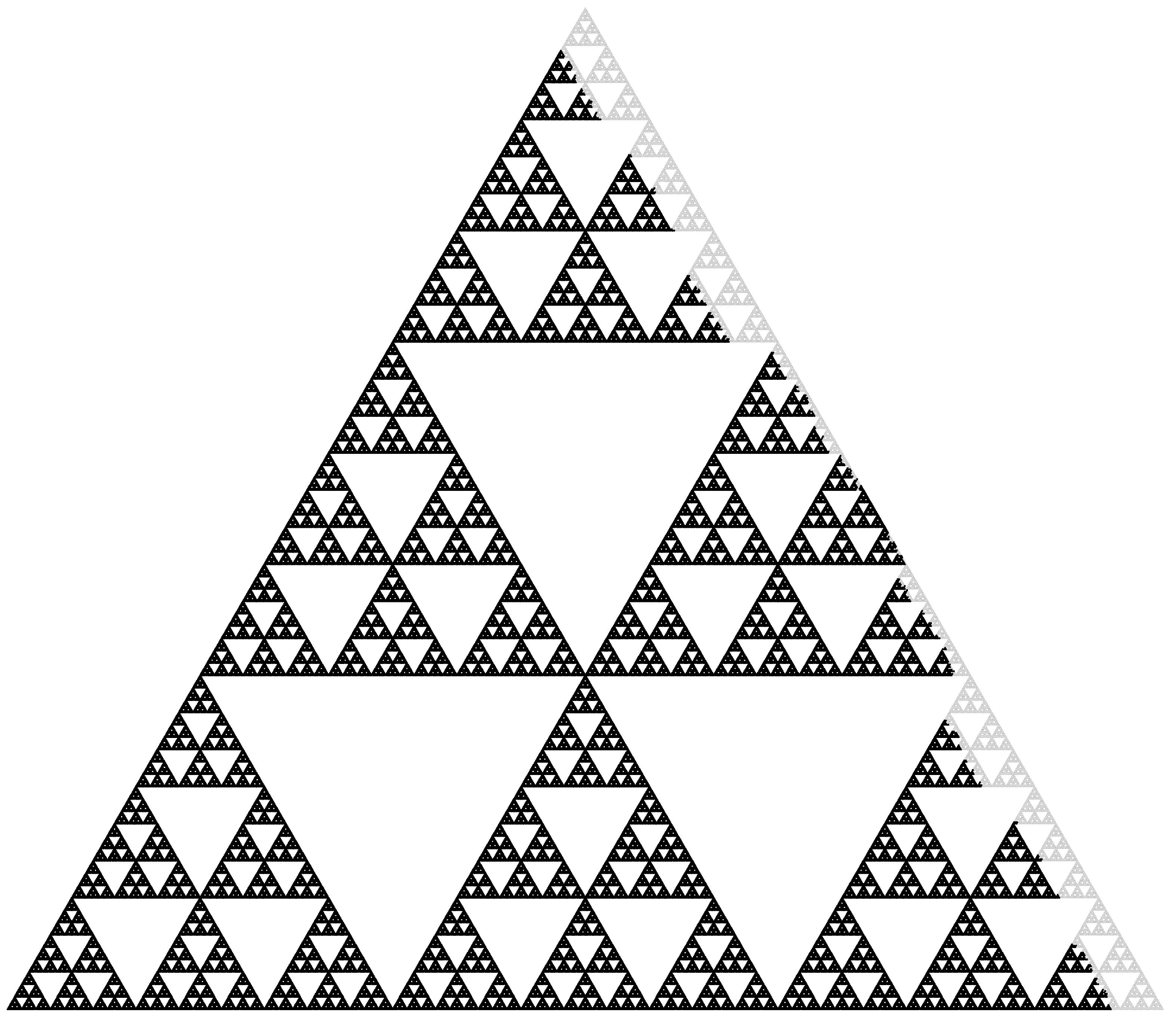
Furthermore, this approach can also be used for other self-similar graphs approximating nested fractals. For example, the graphical approximation of the extension of the Sierpinski gasket to higher dimensions $d\ge 3$ can be extended to a regular graph as we did for $SG$. We also expect the divisible sandpile on this graph to be an exact ball in the graph metric. Evaluating its odometer function, like we did in Section 3, should lead to fluctuation bounds completely analogous to our approach in Section 4 and Section 5. For the Vicsek graph, the graph approximation of the Vicsek set Example 4.1.5 of [21], we also conjecture our technique to work since the divisible sandpile is also an exact ball. Here, the difficulty lies mainly in the additional technicalities and the exact analysis of a normalized odometer function, which is needed since the graph is not regular anymore. We expect this to also generalize to other nested fractals. However, one may need to consider another metric other than the graph metric to describe the shape of the cluster since the harmonic measure on the usual graph metric balls is not uniform anymore. Take a modified Sierpinski gasket graph, where instead of three copies in each stage of the construction, we take nine copies of the triangle in the previous stage. Here, the cluster will grow much faster on the outer middle triangle than on the other ones. Figure 2 shows a simulation on the 6th generation of such a modified Sierpinski gasket graph, where the fluctuation is of the size of a third-generation triangle. Considering infinitely ramified fractals, our approach seems not too promising, as the generations of the approximating graphs are connected on unbounded many vertices. This makes the analysis of the divisible sandpile and its odometer function very hard. See Figure 2 of [16] for a simulation of IDLA clusters on the Sierpinski carpet graph.

References

- Diaconis, P.; Fulton, W. A growth model, a game, an algebra, Lagrange inversion, and characteristic classes. Rend. Sem. Mat. Univ. Pol. Torino 1991, 49, 95–119. [Google Scholar]
- Lawler, G.F.; Bramson, M.; Griffeath, D. Internal diffusion limited aggregation. Ann. Probab. 1992, 20, 2117–2140. [Google Scholar] [CrossRef]
- Lawler, G.F. Subdiffusive fluctuations for internal diffusion limited aggregation. Ann. Probab. 1995, 23, 71–86. [Google Scholar] [CrossRef]
- Asselah, A.; Gaudillière, A. Sublogarithmic fluctuations for internal DLA. Ann. Probab. 2013, 41, 1160–1179. [Google Scholar] [CrossRef] [Green Version]
- Jerison, D.; Levine, L.; Sheffield, S. Internal DLA in higher dimensions. Electron. J. Probab. 2013, 18, 1–14. [Google Scholar] [CrossRef]
- Asselah, A.; Gaudillière, A. From logarithmic to subdiffusive polynomial fluctuations for internal DLA and related growth models. Ann. Probab. 2013, 41, 1115–1159. [Google Scholar] [CrossRef]
- Jerison, D.; Levine, L.; Sheffield, S. Logarithmic fluctuations for internal DLA. J. Amer. Math. Soc. 2012, 25, 271–301. [Google Scholar] [CrossRef] [Green Version]
- Levine, L.; Peres, Y. Scaling limits for internal aggregation models with multiple sources. J. Anal. Math. 2010, 111, 151–219. [Google Scholar] [CrossRef] [Green Version]
- Blachère, S.; Brofferio, S. Internal diffusion limited aggregation on discrete groups having exponential growth. Probab. Theory Related Fields 2007, 137, 323–343. [Google Scholar] [CrossRef] [Green Version]
- Shellef, E. IDLA on the Supercritical Percolation Cluster. Electron. J. Probab. 2010, 15, 723–740. [Google Scholar] [CrossRef]
- Duminil-Copin, H.; Lucas, C.; Yadin, A.; Yehudayoff, A. Containing internal diffusion limited aggregation. Electron. Commun. Probab. 2013, 18, 1–8. [Google Scholar]
- Huss, W.; Sava, E. Internal aggregation models on comb lattices. Electron. J. Probab. 2012, 17, 1–21. [Google Scholar] [CrossRef]
- Asselah, A.; Rahmani, H. Fluctuations for internal DLA on the comb. Ann. Inst. Henri Poincaré Probab. Stat. 2016, 52, 58–83. [Google Scholar] [CrossRef]
- Levine, L.; Silvestri, V. How long does it take for internal DLA to forget its initial profile. Probab. Theory Related Fields 2019, 174, 1219–1271. [Google Scholar] [CrossRef] [Green Version]
- Sava-Huss, E. From Fractals in External DLA to Internal DLA on Fractals. In Fractal Geometry and Stochastics VI; Freiberg, U., Hambly, B., Hinz, M., Winter, S., Eds.; Birkhäuser: Basel, Switzerland, 2021; pp. 273–298. ISBN 978-3-030-59651-4. [Google Scholar]
- Chen, J.P.; Huss, W.; Sava-Huss, E.; Teplyaev, A. Internal DLA on Sierpinski gasket graphs. In Analysis and Geometry on Graphs and Manifolds; Keller, M., Lenz, D., Wojciechowski, R.K., Eds.; Cambridge University Press: Cambridge, UK, 2020; pp. 126–155. [Google Scholar]
- Chen, J.P.; Kudler-Flam, J. Laplacian growth and sandpiles on the Sierpiński gasket: Limit shape universality and exact solutions. Ann. Inst. Henri Poincaré D 2020, 7, 585–664. [Google Scholar] [CrossRef] [PubMed]
- Huss, W.; Sava-Huss, E. Divisible sandpile on Sierpinski gasket graphs. Fractals 2019, 27, 1950032. [Google Scholar] [CrossRef] [Green Version]
- Barlow, M.T.; Perkins, E.A. Brownian motion on the Sierpinski gasket. Probab. Theory Related Fields 1988, 79, 543–623. [Google Scholar] [CrossRef]
- Kigami, J. Analysis on Fractals; Cambridge University Press: Cambridge, UK, 2001; ISBN 978-0-5217-9321-6. [Google Scholar]
- Strichartz, R.S. Differential Equations on Fractals: A Tutorial; Princeton University Press: Princeton, NJ, USA, 2006; ISBN 978-0-6911-2731-6. [Google Scholar]
- Teplyaev, A. Spectral Analysis on Infinite Sierpiński Gaskets. J. Funct. Anal. 1998, 159, 537–567. [Google Scholar] [CrossRef] [Green Version]
- Grabner, P.J.; Woess, W. Functional iterations and periodic oscillations for simple random walk on the Sierpiński graph. Stochastic Process. Appl. 1997, 69, 127–138. [Google Scholar] [CrossRef] [Green Version]
- Jones, O.D. Transition probabilities for the simple random walk on the Sierpinski graph. Stochastic Process. Appl. 1996, 61, 45–69. [Google Scholar] [CrossRef] [Green Version]
- Teufl, E. The average displacement of the simple random walk on the Sierpiński graph. Combin. Probab. Comput. 2003, 12, 203–222. [Google Scholar] [CrossRef]
- Hattori, K.; Mizuno, M. Loop-erased random walk on the Sierpinski gasket. Stochastic Process. Appl. 2014, 124, 566–585. [Google Scholar] [CrossRef]
- Shinoda, M.; Teufl, E.; Wagner, S. Uniform spanning trees on Sierpinski graphs. Lat. Am. J. Probab. Math. Stat. 2014, 11, 737–780. [Google Scholar]
- Hinz, A.M.; Schief, A. The average distance on the Sierpiński gasket. Probab. Theory Related Fields 1990, 87, 129–138. [Google Scholar] [CrossRef]
- Chang, S.; Chen, L.; Yang, W. Spanning trees on the Sierpinski gasket. J. Stat. Phys. 2007, 126, 649–667. [Google Scholar] [CrossRef] [Green Version]
- Teufl, E.; Wagner, S. The number of spanning trees in self-similar graphs. Ann. Comb. 2011, 15, 355. [Google Scholar] [CrossRef]
- Caldarola, F. The exact measures of the Sierpiński d-dimensional tetrahedron in connection with a Diophantine nonlinear system. Commun. Nonlinear Sci. Numer. Simul. 2018, 63, 228–238. [Google Scholar] [CrossRef]
- Hattori, K.; Hattori, T.; Kusuoka, S. Self-avoiding paths on the three dimensional Sierpinski gasket. Publ. Res. Inst. Math. Sci. 1993, 29, 455–509. [Google Scholar] [CrossRef] [Green Version]
- Cristea, L.L.; Steinsky, B. Distances in Sierpiński graphs and on the Sierpiński gasket. Aequationes Math. 2013, 85, 201–219. [Google Scholar] [CrossRef]
- Levine, L.; Peres, Y. Strong spherical asymptotics for rotor-router aggregation and the divisible sandpile. Potential Anal. 2009, 30, 1–27. [Google Scholar] [CrossRef] [Green Version]
- Barlow, M.T. Heat kernels and sets with fractal structure. Contemp. Math. 2003, 338, 11–40. [Google Scholar]
Figure 1.
The double sided Sierpinski gasket graph as illustrated in Figure 1 of [16].
Figure 2.
Simulation on the modified Sierpinski gasket graph with nine copies.
Disclaimer/Publisher’s Note: The statements, opinions and data contained in all publications are solely those of the individual author(s) and contributor(s) and not of MDPI and/or the editor(s). MDPI and/or the editor(s) disclaim responsibility for any injury to people or property resulting from any ideas, methods, instructions or products referred to in the content. |
© 2023 by the author. Licensee MDPI, Basel, Switzerland. This article is an open access article distributed under the terms and conditions of the Creative Commons Attribution (CC BY) license (https://creativecommons.org/licenses/by/4.0/).
Share and Cite
MDPI and ACS Style
Heizmann, N. On the Fluctuations of Internal DLA on the Sierpinski Gasket Graph. Math. Comput. Appl. 2023, 28, 73. https://doi.org/10.3390/mca28030073
AMA Style
Heizmann N. On the Fluctuations of Internal DLA on the Sierpinski Gasket Graph. Mathematical and Computational Applications. 2023; 28(3):73. https://doi.org/10.3390/mca28030073
Chicago/Turabian StyleHeizmann, Nico. 2023. "On the Fluctuations of Internal DLA on the Sierpinski Gasket Graph" Mathematical and Computational Applications 28, no. 3: 73. https://doi.org/10.3390/mca28030073