
Intermediate Encoding Layers for the Generative Design of 2D Soft Robot Actuators: A Comparison of CPPN’s, L-Systems and Random Generation

Abstract
:1. Introduction
2. Methods and Materials
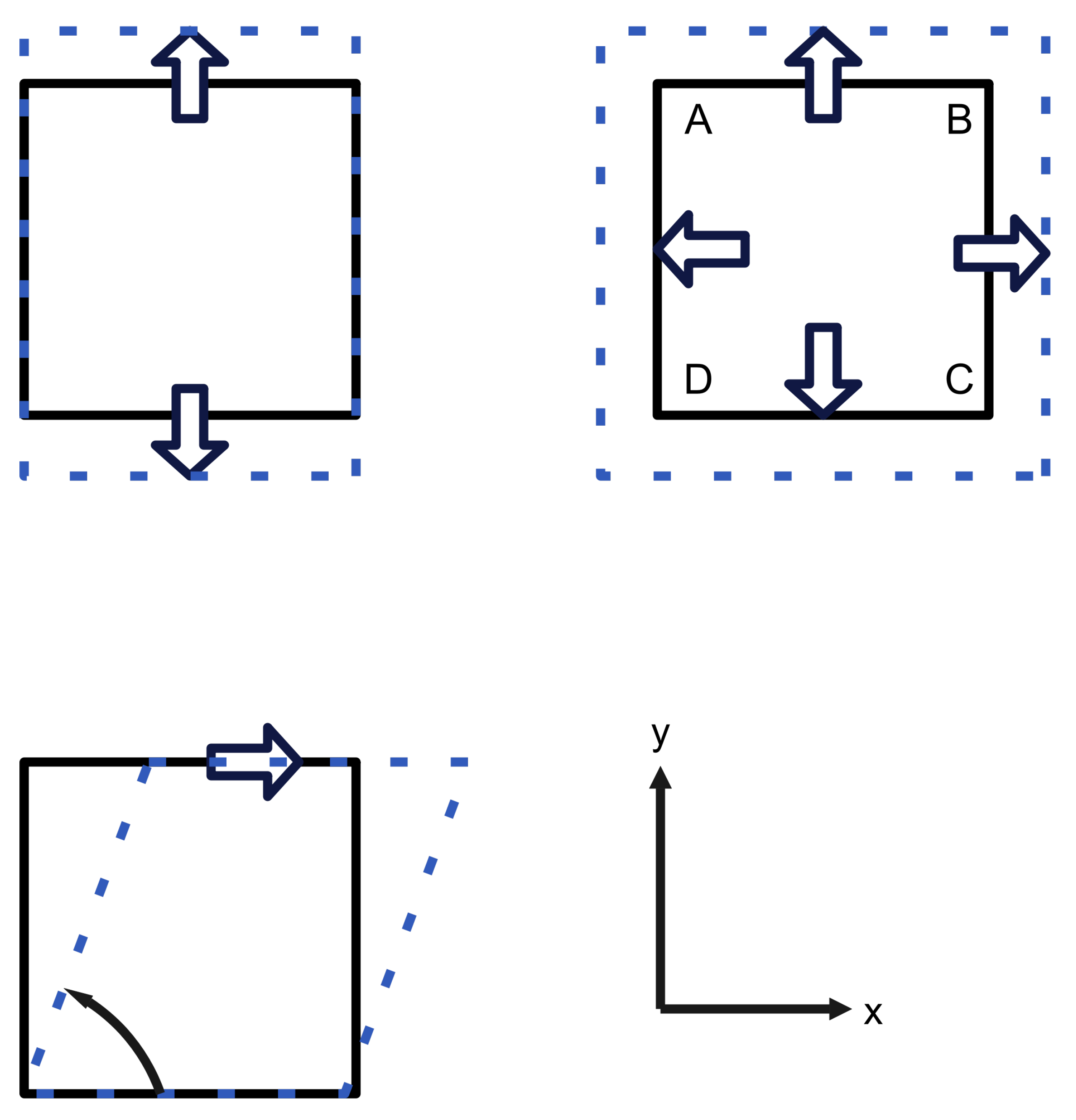
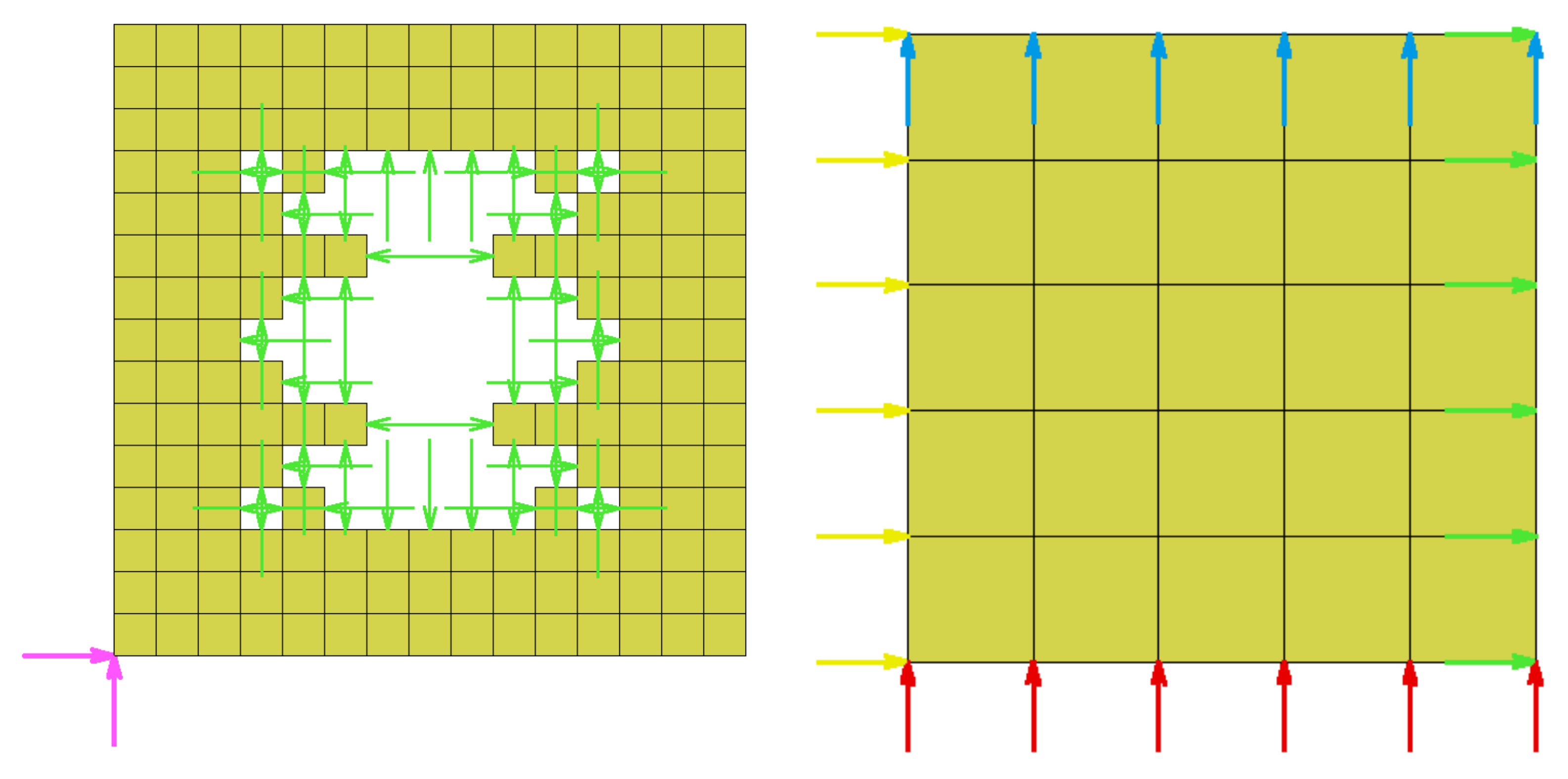
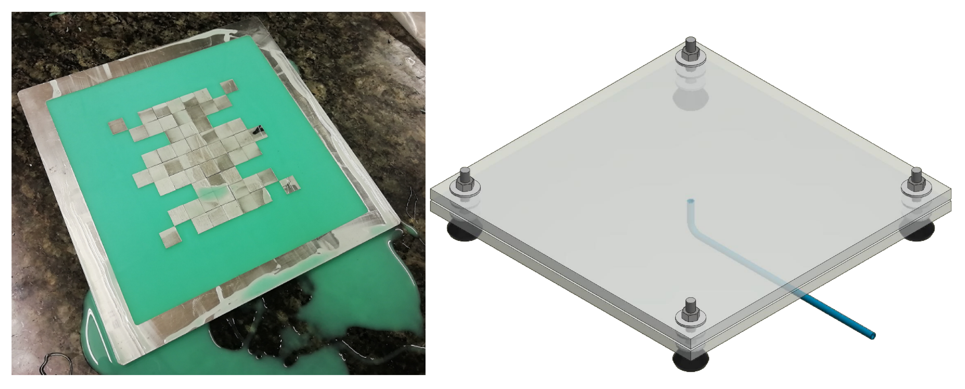
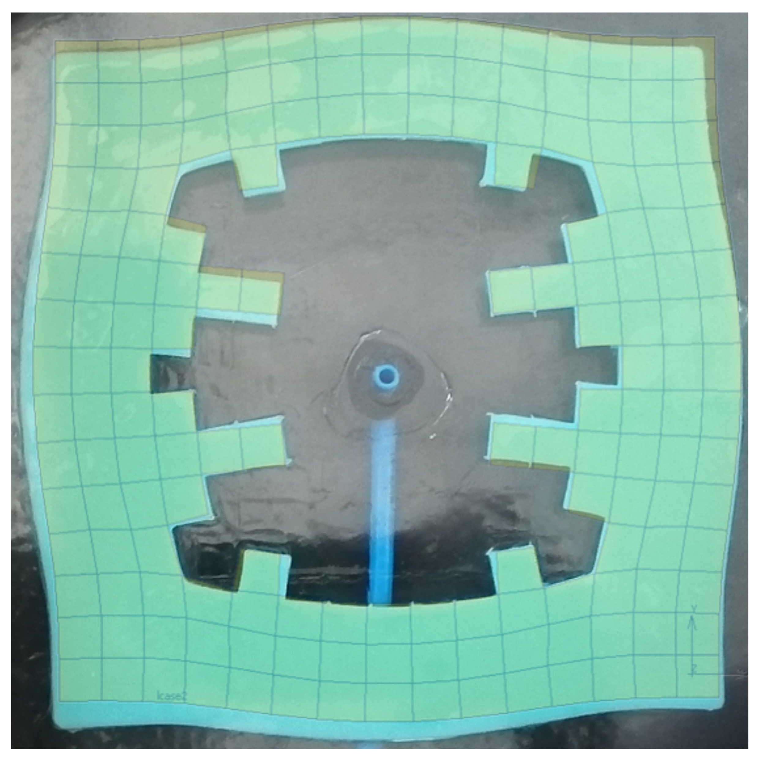
2.1. Test Case
2.2. Encoding Methods
2.2.1. Random Units
2.2.2. Lindenmayer Systems
2.2.3. Compositional Pattern Producing Networks
3. Results and Analysis
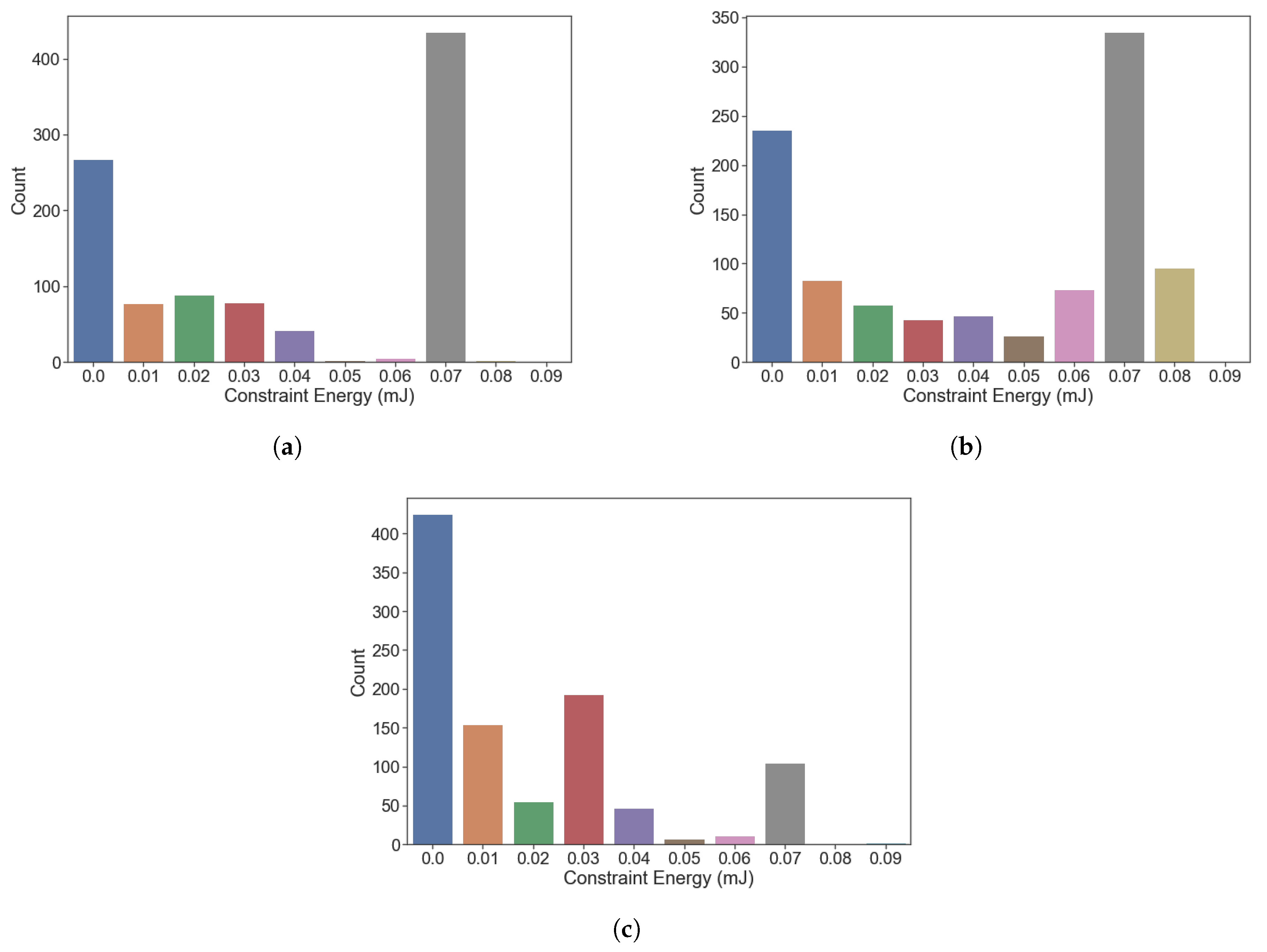
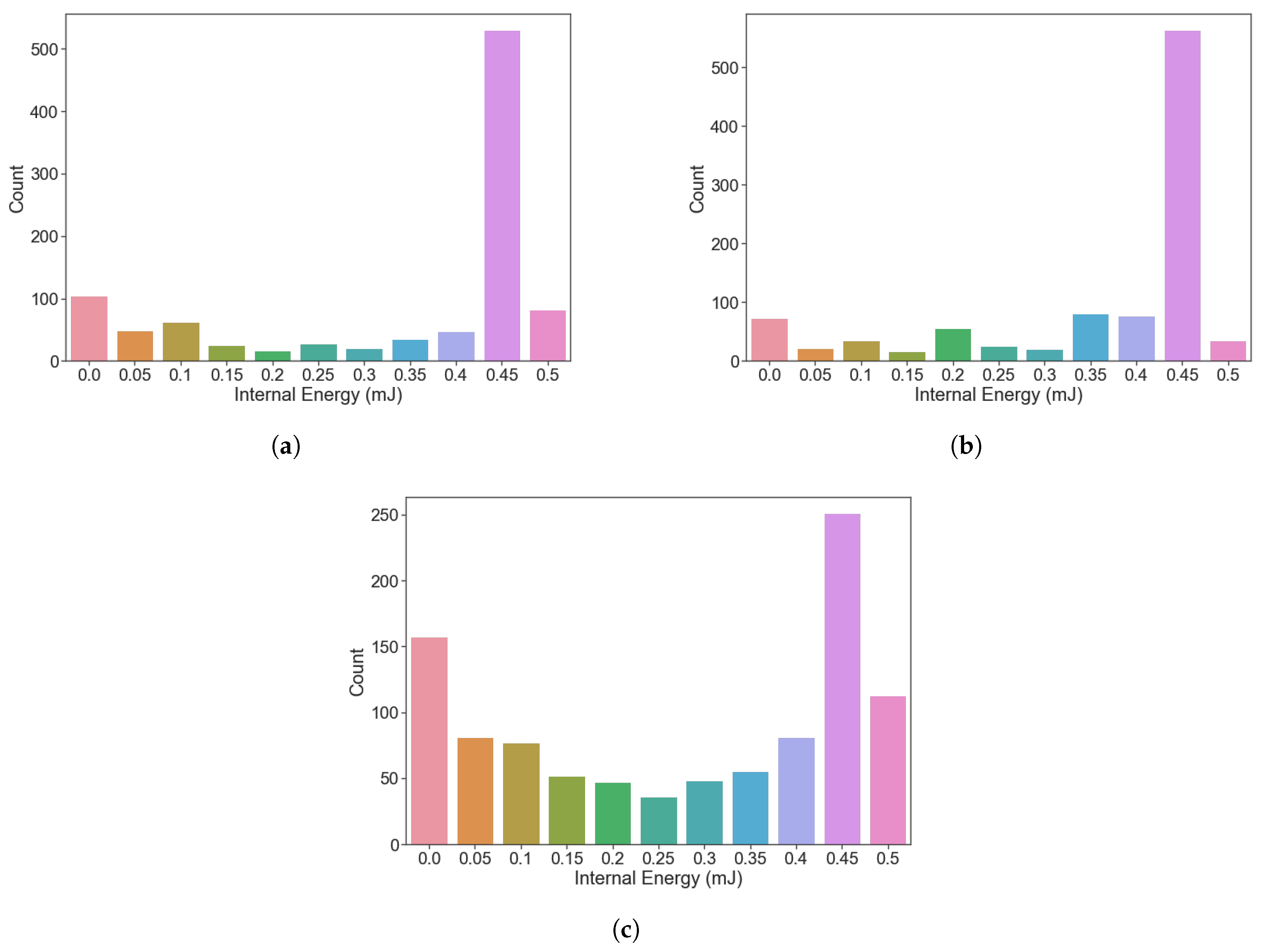
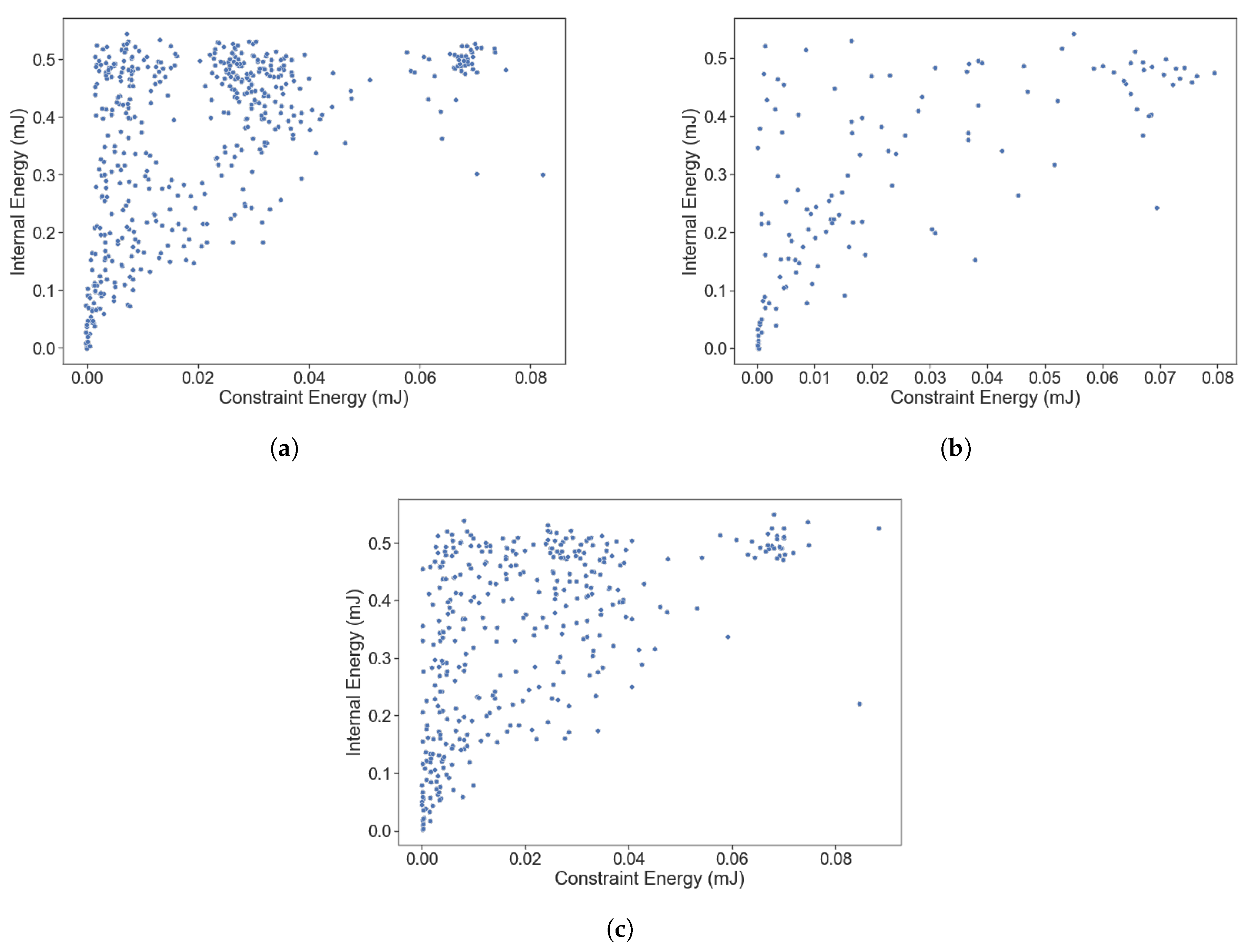
- 1.
- High constraint energy, high internal energy—Units that do not deform to the desired shape and require significant work to maintain that shape.
- 2.
- High constraint energy, low internal energy—Units that do not deform to the desired shape but do not require much work to maintain that shape.
- 3.
- Low constraint energy, low internal energy—Units that deform to the desired shape and do not require much work to maintain that shape.
- 4.
- Low constraint energy, high internal energy—Units that deform to the desired shape but require significant work to maintain that shape.
4. Conclusions
Author Contributions
Funding
Data Availability Statement
Conflicts of Interest
References
- Rus, D.; Tolley, M. Design, fabrication and control of soft robots. Nature 2015, 521, 467–475. [Google Scholar] [CrossRef]
- Mengaldo, G.; Renda, F.; Brunton, S.L.; Bächer, M.; Calisti, M.; Duriez, C.; Chirikjian, G.S.; Laschi, C. A concise guide to modelling the physics of embodied intelligence in soft robotics. Nat. Rev. Phys. 2022, 4, 595–610. [Google Scholar] [CrossRef]
- Iida, F.; Laschi, C. Soft robotics: Challenges and perspectives. Procedia Comput. 2011, 7, 99–102. [Google Scholar] [CrossRef]
- Howison, T.; Hauser, S.; Hughes, J.; Iida, F. Reality-Assisted Evolution of Soft Robots through Large-Scale Physical Experimentation: A Review. Artif 2021, 26, 484–506. [Google Scholar] [CrossRef]
- Laschi, C.; Mazzolai, B.; Cianchetti, M. Soft robotics: Technologies and systems pushing the boundaries of robot abilities. Sci. Robot. 2016, 1, eaah3690. [Google Scholar] [CrossRef] [PubMed]
- Armanini, C.; Boyer, F.; Mathew, A.; Duriez, C.; Renda, F. Soft Robots Modeling: A Structured Overview. IEEE Trans. Robot. 2023, 1–21. [Google Scholar] [CrossRef]
- Chen, W.; Wu, S.; Zhou, T.; Xiong, C. On the biological mechanics and energetics of the hip joint muscle–tendon system assisted by passive hip exoskeleton. Bioinspir Biomim 2018, 14, 016012. [Google Scholar] [CrossRef] [PubMed]
- Pagoli, A.; Chapelle, F.; Corrales-Ramon, J.; Mezouar, Y.; Lapusta, Y. Review of soft fluidic actuators: Classification and materials modeling analysis. SMS 2022, 31, 013001. [Google Scholar] [CrossRef]
- Ilievski, F.; Mazzeo, A.; Shepherd, R.; Chen, X.; Whitesides, G. Soft Robotics for Chemists. Angew. Chem. Int. Ed. 2011, 123, 1930–1935. [Google Scholar] [CrossRef]
- Shepherd, R.; Ilievski, F.; Choi, W.; Morin, S.; Stokes, A.; Mazzeo, A.; Chen, X.; Wang, M.; Whitesides, G. Multigait soft robot. Proc. Natl. Acad. Sci. USA 2011, 108, 20400–20403. [Google Scholar] [CrossRef]
- Mosadegh, B.; Polygerinos, P.; Keplinger, C.; Wennstedt, S.; Shepherd, R.; Gupta, U.; Shim, J.; Bertoldi, K.; Walsh, C.; Whitesides, G. Pneumatic networks for soft robotics that actuate rapidly. Adv. Funct. Mater. 2014, 24, 2163–2170. [Google Scholar] [CrossRef]
- Mutlu, R.; Alici, G.; Li, W. Electroactive polymers as soft robotic actuators: Electro-mechanical modeling and identification. In Proceedings of the 2013 IEEE/ASME International Conference on Advanced Intelligent Mechatronics, Wollongong, NSW, Australia, 9–12 July 2013; pp. 1096–1101. [Google Scholar]
- Laschi, C.; Cianchetti, M. Soft robotics: New perspectives for robot bodyware and control. Front. Bioeng. Biotechnol. 2014, 2, 3. [Google Scholar] [CrossRef]
- Olsen, Z.; Kim, K. Design and Modeling of a New Biomimetic Soft Robotic Jellyfish Using IPMC-Based Electroactive Polymers. Front. Robot. AI 2019, 6, 112. [Google Scholar] [CrossRef]
- Paez, L.; Agarwal, G.; Paik, J. Design and Analysis of a Soft Pneumatic Actuator with Origami Shell Reinforcement. Soft Robot. 2016, 3, 109–119. [Google Scholar] [CrossRef]
- Yi, J.; Chen, X.; Song, C.; Zhou, J.; Liu, Y.; Liu, S.; Wang, Z. Customizable Three-Dimensional-Printed Origami Soft Robotic Joint with Effective Behavior Shaping for Safe Interactions. IEEE Trans. Robot. 2019, 35, 114–123. [Google Scholar] [CrossRef]
- Ze, Q.; Wu, S.; Nishikawa, J.; Dai, J.; Sun, Y.; Leanza, S.; Zemelka, C.; Novelino, L.; Paulino, G.; Zhao, R. Soft robotic origami crawler. Sci. Adv. 2022, 8, 7834. [Google Scholar] [CrossRef]
- Jin, H.; Dong, E.; Xu, M.; Liu, C.; Alici, G.; Jie, Y. Soft and smart modular structures actuated by shape memory alloy (SMA) wires as tentacles of soft robots. SMS 2016, 25, 085026. [Google Scholar] [CrossRef]
- Copaci, D.; Cano, E.; Moreno, L.; Blanco, D. New Design of a Soft Robotics Wearable Elbow Exoskeleton Based on Shape Memory Alloy Wire Actuators. Appl. Bionics Biomech. 2017, 2017, 1605101. [Google Scholar] [CrossRef] [PubMed]
- Rodrigue, H.; Wang, W.; Han, M.; Kim, T.; Ahn, S. An Overview of Shape Memory Alloy-Coupled Actuators and Robots. Soft Robot. 2017, 4, 3–15. [Google Scholar] [CrossRef] [PubMed]
- Wang, W.; Ahn, S. Shape Memory Alloy-Based Soft Gripper with Variable Stiffness for Compliant and Effective Grasping. Soft Robot. 2017, 4, 379–389. [Google Scholar] [CrossRef]
- Stokes, A.; Shepherd, R.; Morin, S.; Ilievski, F.; Whitesides, G. A Hybrid Combining Hard and Soft Robots. Soft Robot. 2014, 1, 70–74. [Google Scholar] [CrossRef]
- Patino, T.; Mestre, R.; Sánchez, S. Miniaturised soft bio-hybrid robotics: A step forward into healthcare applications. Lab Chip 2016, 16, 3626–3630. [Google Scholar] [CrossRef]
- Rich, S.; Wood, R.; Majidi, C. Untethered soft robotics. Nat. Electron. 2018, 1, 102–112. [Google Scholar] [CrossRef]
- Stano, G.; Percoco, G. Additive manufacturing aimed to soft robots fabrication: A review. Extreme Mech. Lett. 2021, 42, 101079. [Google Scholar] [CrossRef]
- Cianchetti, M.; Laschi, C.; Menciassi, A.; Dario, P. Biomedical applications of soft robotics. Nat. Rev. Mater. 2018, 3, 143–153. [Google Scholar] [CrossRef]
- Gifari, M.; Naghibi, H.; Stramigioli, S.; Abayazid, M. A review on recent advances in soft surgical robots for endoscopic applications. Int. J. Med. Robot. 2019, 15, e2010. [Google Scholar] [CrossRef]
- Runciman, M.; Darzi, A.; Mylonas, G. Soft Robotics in Minimally Invasive Surgery. Soft Robot. 2019, 6, 423–443. [Google Scholar] [CrossRef] [PubMed]
- Albu-Schaffer, A.; Eiberger, O.; Grebenstein, M.; Haddadin, S.; Ott, C.; Wimböck, T.; Wolf, S.; Hirzinger, G. Soft robotics. IEEE Robot. Autom. Mag. 2008, 15, 20–30. [Google Scholar] [CrossRef]
- Glick, P.; Suresh, S.; Ruffatto, D.; Cutkosky, M.; Tolley, M.; Parness, A. A Soft Robotic Gripper with Gecko-Inspired Adhesive. IEEE Robot. Autom. Lett 2018, 3, 903–910. [Google Scholar] [CrossRef]
- Boyraz, P.; Runge, G.; Raatz, A. An overview of novel actuators for soft robotics. High-Throughput 2018, 7, 48. [Google Scholar] [CrossRef]
- Sun, Z.; Zhu, M.; Zhang, Z.; Chen, Z.; Shi, Q.; Shan, X.; Yeow, R.; Lee, C. Artificial Intelligence of Things (AIoT) Enabled Virtual Shop Applications Using Self-Powered Sensor Enhanced Soft Robotic Manipulator. Adv. Sci. 2021, 8, 2100230. [Google Scholar] [CrossRef]
- Zhang, C.; Zhu, P.; Lin, Y.; Jiao, Z.; Zou, J. Modular SoAuthors need to follow the proper guideline for the referencing formats provided by MDPI MCA journal. Do not add the DOI of journals and conference articles, if not required. Change made as advised. ft Robotics: Modular Units, Connection Mechanisms, and Applications. Adv. Intel. 2020, 2, 1900166. [Google Scholar]
- Polygerinos, P.; Correll, N.; Morin, S.; Mosadegh, B.; Onal, C.; Petersen, K.; Cianchetti, M.; Tolley, M.; Shepherd, R. Soft Robotics: Review of Fluid-Driven Intrinsically Soft Devices; Manufacturing, Sensing, Control, and Applications in Human-Robot Interaction. Adv. Eng. Mater. 2017, 19, 1700016. [Google Scholar] [CrossRef]
- Arnold, T.; Scheutz, M. The tactile ethics of soft robotics: Designing wisely for human–robot interaction. Soft Robot. 2017, 4, 81–87. [Google Scholar] [CrossRef] [PubMed]
- Das, A.; Nabi, M. A review on Soft Robotics: Modeling, Control and Applications in Human-Robot Interaction. In Proceedings of the International Conference on Computing, Communication, and Intelligent Systems, Greater Noida, India, 18–19 October 2019; pp. 306–311. [Google Scholar]
- Xiong, J.; Chen, J.; Lee, P. Functional Fibers and Fabrics for Soft Robotics, Wearables, and Human-Robot Interface. Adv. Mater. 2021, 33, 2002640. [Google Scholar] [CrossRef]
- Jørgensen, J.; Bojesen, K.; Jochum, E. Is a Soft Robot More “Natural”? Exploring the Perception of Soft Robotics in Human-Robot Interaction. Int. J. Soc. Robot. 2022, 14, 95–113. [Google Scholar] [CrossRef]
- Rossiter, J.; Winfield, J.; Ieropoulos, I. Here today, gone tomorrow: Biodegradable soft robots. In Proceedings of the Electroactive Polymer Actuators and Devices, Las Vegas, NV, USA, 20–24 March 2016. [Google Scholar]
- Mazzolai, B.; Kraus, T.; Pirrone, N.; Kooistra, L.; Simone, A.; Cottin, A.; Margheri, L. Towards new frontiers for distributed environmental monitoring based on an ecosystem of plant seed-like soft robots. In Proceedings of the 2021 Conference on Information Technology For Social Good, Roma, Italy, 9–11 September 2021; pp. 221–224. [Google Scholar]
- Karmakar, S.; Sarkar, A. Design and implementation of bio-inspired soft robotic grippers. In Proceedings of the Advances in Robotics, Chennai, India, 2–6 July 2019; pp. 1–6. [Google Scholar]
- Joshi, A.; Kulkarni, A.; Tadesse, Y. FludoJelly: Experimental study on jellyfish-like soft robot enabled by soft pneumatic composite (SPC). Robotics 2019, 8, 56. [Google Scholar] [CrossRef]
- Soon, H.; Rosli, N.; Athif, A.; Faudzi, M. Design and control of biomimicry eye using soft actuator. PERINTIS EJournal 2020, 10, 34–49. [Google Scholar]
- Park, C.; Fan, Y.; Hager, G.; Yuk, H.; Singh, M.; Rojas, A.; Hameed, A.; Saeed, M.; Vasilyev, N.; Steele, T.; et al. An organosynthetic dynamic heart model with enhanced biomimicry guided by cardiac diffusion tensor imaging. Sci. Robot. 2020, 5, eaay9106. [Google Scholar] [CrossRef] [PubMed]
- Youssef, S.; Soliman, M.; Saleh, M.; Mousa, M.; Elsamanty, M.; Radwan, A. Underwater Soft Robotics: A Review of Bioinspiration in Design, Actuation, Modeling, and Control. Micromachines 2022, 13, 110. [Google Scholar] [CrossRef]
- Stuttaford-Fowler, A.; Samani, H.; Yang, C. Biomimicry in Soft Robotics Actuation and Locomotion. In Proceedings of the International Conference On System Science and Engineering, Taichung, Taiwan, 26–29 May 2022; pp. 17–21. [Google Scholar]
- Dong, X.; Luo, X.; Zhao, H.; Qiao, C.; Li, J.; Yi, J.; Yang, L.; Oropeza, F.; Hu, T.; Xu, Q.; et al. Recent advances in biomimetic soft robotics: Fabrication approaches, driven strategies and applications. Soft Matter 2022, 18, 7699–7734. [Google Scholar] [CrossRef] [PubMed]
- Sun, J.; Bauman, L.; Yu, L.; Zhao, B. Gecko-and-inchworm-inspired untethered soft robot for climbing on walls and ceilings. Cell Rep. 2023, 4, 101241. [Google Scholar] [CrossRef]
- Maur, P.; Djambazi, B.; Haberthur, Y.; Hormann, P.; Kubler, A.; Lustenberger, M.; Sigrist, S.; Vigen, O.; Forster, J.; Achermann, F.; et al. RoBoa: Construction and evaluation of a steerable vine robot for search and rescue applications. In Proceedings of the 4th International Conference On Soft Robotics, New Haven, CT, USA, 2–16 April 2021; pp. 15–20. [Google Scholar]
- Jørgensen, J. Leveraging morphological computation for expressive movement generation in a soft robotic artwork. In Proceedings of the ACM International Conference Proceeding Series, London, UK, 28–30 June 2017; pp. 1–4. [Google Scholar]
- Lee, J.; Eom, J.; Choi, W.; Cho, K. Soft LEGO: Bottom-up Design Platform for Soft Robotics. In Proceedings of the IEEE/RSJ International Conference on Intelligent Robots and Systems, Madrid, Spain, 1–5 October 2018; pp. 7513–7520. [Google Scholar]
- Pinskier, J.; Howard, D. From Bioinspiration to Computer Generation: Developments in Autonomous Soft Robot Design. Adv. Intel. 2022, 4, 2100086. [Google Scholar] [CrossRef]
- Wang, H.; Totaro, M.; Beccai, L. Toward Perceptive Soft Robots: Progress and Challenges. Adv. Sci. 2018, 5, 1800541. [Google Scholar] [CrossRef]
- Chen, F.; Wang, M. Design Optimization of Soft Robots: A Review of the State of the Art. IEEE Robot. Autom. Mag. 2020, 27, 27–43. [Google Scholar] [CrossRef]
- Lipson, H.; Pollack, J. Automatic design and manufacture of robotic lifeforms. Nature 2000, 406, 974–978. [Google Scholar] [CrossRef] [PubMed]
- Hiller, J.; Lipson, H. Automatic design and manufacture of soft robots. IEEE Trans. Robot. 2012, 28, 457–466. [Google Scholar] [CrossRef]
- Ellis, D.; Venter, M.; Venter, G. Computational design for inflated shape of a modular soft robotic actuator. In Proceedings of the IEEE International Conference on Soft Robotics, Seoul, Republic of Korea, 14–18 April 2019; pp. 7–12. [Google Scholar]
- Conradie, N. A Scale-Invariant Generative Design Process for 2D Soft Robot Actuators. Ph.D. Thesis, Stellenbosch University, Stellenbosch, South Africa, 2021. [Google Scholar]
- Ellis, D.; Venter, M.; Venter, G. Generative Design Procedure for Embedding Specified Planar Behavior in Modular Soft Pneumatic Actuators. Soft Robot. 2022, 9, 552–561. [Google Scholar] [CrossRef]
- Pinskier, J.; Shirinzadeh, B. Topology optimisation of leaf flexures to maximise in-plane to out-of-plane compliance ratio. Precis. Eng. 2019, 55, 397–407. [Google Scholar] [CrossRef]
- Sun, Y.; Liu, Y.; Pancheri, F.; Lueth, T.C. LARG: A Lightweight Robotic Gripper with 3-D Topology Optimised Adaptive Fingers. IEEE ASME Trans. Mechatron. 2022, 27, 2026–2034. [Google Scholar] [CrossRef]
- Venter, M.P.; Joubert, I.J. Generative Design of Soft Robot Actuators Using ESP. Math. Comput. Appl. 2023, 28, 53. [Google Scholar] [CrossRef]
- Lai, G.; Leymarie, F.; Latham, W.; Arita, T.; Suz’uki, R. Virtual Creature Morphology—A Review. Comput. Graph Forum 2021, 40, 659–681. [Google Scholar] [CrossRef]
- Choi, H.; Crump, C.; Duriez, C.; Elmquist, A.; Hager, G.; Han, D.; Hearl, F.; Hodgins, J.; Jain, A.; Leve, F.; et al. On the use of simulation in robotics: Opportunities, challenges, and suggestions for moving forward. Proc. Natl. Acad. Sci. USA 2023, 118, e1907856118. [Google Scholar] [CrossRef]
- Xavier, M.S.; Fleming, A.J.; Yong, Y.K. Finite Element Modeling of Soft Fluidic Actuators: Overview and Recent Developments. Adv. Intell. Syst. 2021, 3, 2000187. [Google Scholar] [CrossRef]
- Marechal, L.; Balland, P.; Lindenroth, L.; Petrou, F.; Kontovounisios, C.; Bello, F. Toward a Common Framework and Database of Materials for Soft Robotics. SoRo 2021, 8, 284–297. [Google Scholar] [CrossRef]
- Tanaka, H.; Leon-garcia, A. Efficient Run-Length Encodings. IEEE Trans. Inf. Theory 1982, 28, 880–890. [Google Scholar] [CrossRef]
- Javed, M.; Nadeem, A. Data compression through adaptive Huffman coding scheme. In Proceedings of the 2000 TENCON Proceedings. Intelligent Systems and Technologies for the New Millennium, Kuala Lumpur, Malaysia, 24–27 September 2000; pp. 187–190. [Google Scholar]
- Rissanen, J.; Langdon, G. Arithmetic Coding. IBM J. Res. Dev. 1979, 23, 149–162. [Google Scholar] [CrossRef]
- Barnsley, M.; Demko, S. Iterated function systems and the global construction of fractals. Proc. Math. Phys. Eng. Sci. 1985, 399, 243–275. [Google Scholar]
- Lindenmayer, A. L-systems in their biological context. In Proceedings of the 1974 Conference On Biologically Motivated Automata Theory, McLean, VA, USA, 19–21 June 1974; pp. 65–69. [Google Scholar]
- Mandelbrot, B. Fractals; Freeman: San Francisco, CA, USA, 1977. [Google Scholar]
- Wolfram, S. Cellular automata as models of complexity. Nature 1984, 311, 419–424. [Google Scholar] [CrossRef]
- Holland, J. Genetic algorithms. Sci. Am. 1992, 267, 66–73. [Google Scholar] [CrossRef]
- Kennedy, J. Swarm Intelligence; Springer: Berlin/Heidelberg, Germany, 2006. [Google Scholar]
- Turk, G. Generating textures on arbitrary surfaces using reaction-diffusion. ACM Siggraph Comput. Graph. 1991, 25, 289–298. [Google Scholar] [CrossRef]
- Minsky, M. Theory of Neural-Analog Reinforcement Systems and Its Application to the Brain-Model Problem. Ph.D. Thesis, Princeton University, Princeton, NJ, USA, 1954. [Google Scholar]
- Kriegman, S.; Nasab, A.; Blackiston, D.; Steele, H.; Levin, M.; Kramer-Bottiglio, R.; Bongard, J. Scale invariant robot behavior with fractals. arXiv 2021, arXiv:2103.04876. [Google Scholar]
- Cheney, N.; Lipson, H. Topological evolution for embodied cellular automata. J. Theor. 2016, 633, 19–27. [Google Scholar] [CrossRef]
- Giorgio-Serchi, F.; Arienti, A.; Corucci, F.; Giorelli, M.; Laschi, C. Hybrid parameter identification of a multi-modal underwater soft robot. Bioinspir. Biomim. 2017, 12, 025007. [Google Scholar] [CrossRef] [PubMed]
- Terrile, S.; López, A.; Barrientos, A. Use of Finite Elements in the Training of a Neural Network for the Modeling of a Soft Robot. Biomimetics 2023, 8, 56. [Google Scholar] [CrossRef] [PubMed]
- Lassner, M. Graph Embedding Algorithms and Their Applications. Ph.D. Thesis, Wayne State University, Detroit, MI, USA, 1981. [Google Scholar]
- Lucas, M.; Laplaze, L.; Bennett, M. Plant systems biology: Network matters. Plant Cell Environ. 2011, 34, 535–553. [Google Scholar] [CrossRef]
- Ebert, D. Advanced Modeling Techniques for Computer Graphics. ACM Comput. Surv. 1996, 28, 154–156. [Google Scholar] [CrossRef]
- Wonka, P.; Wimmer, M.; Sillion, F.; Ribarsky, W. Instant Architecture. ACM Trans. Graph. 2003, 22, 669–677. [Google Scholar] [CrossRef]
- Stanley, K. Compositional pattern producing networks: A novel abstraction of development. Genet. Program. Evolvable Mach. 2007, 8, 131–162. [Google Scholar] [CrossRef]
- Gu, Y.; Zhang, X.; Wu, Q.; Li, Y.; Zhang, B.; Gao, F.; Luo, Y. Research on motion evolution of soft robot based on VoxCAD. In Proceedings of the Intelligent Robotics and Applications: 12th International Conference, Shenyang, China, 8–11 August 2019; pp. 26–37. [Google Scholar]
- Cheney, N.; Maccurdy, R.; Clune, J.; Lipson, H. Unshackling Evolution: Evolving Soft Robots with Multiple Materials and a Powerful Generative Encoding. ACM SIGEVOlution 2014, 7, 11–23. [Google Scholar] [CrossRef]


| Variables: | F |
| Constants: | [, ], +, −, f |
| Axiom: | F |
| Production Rules: | F → F[−fF][+fF] |
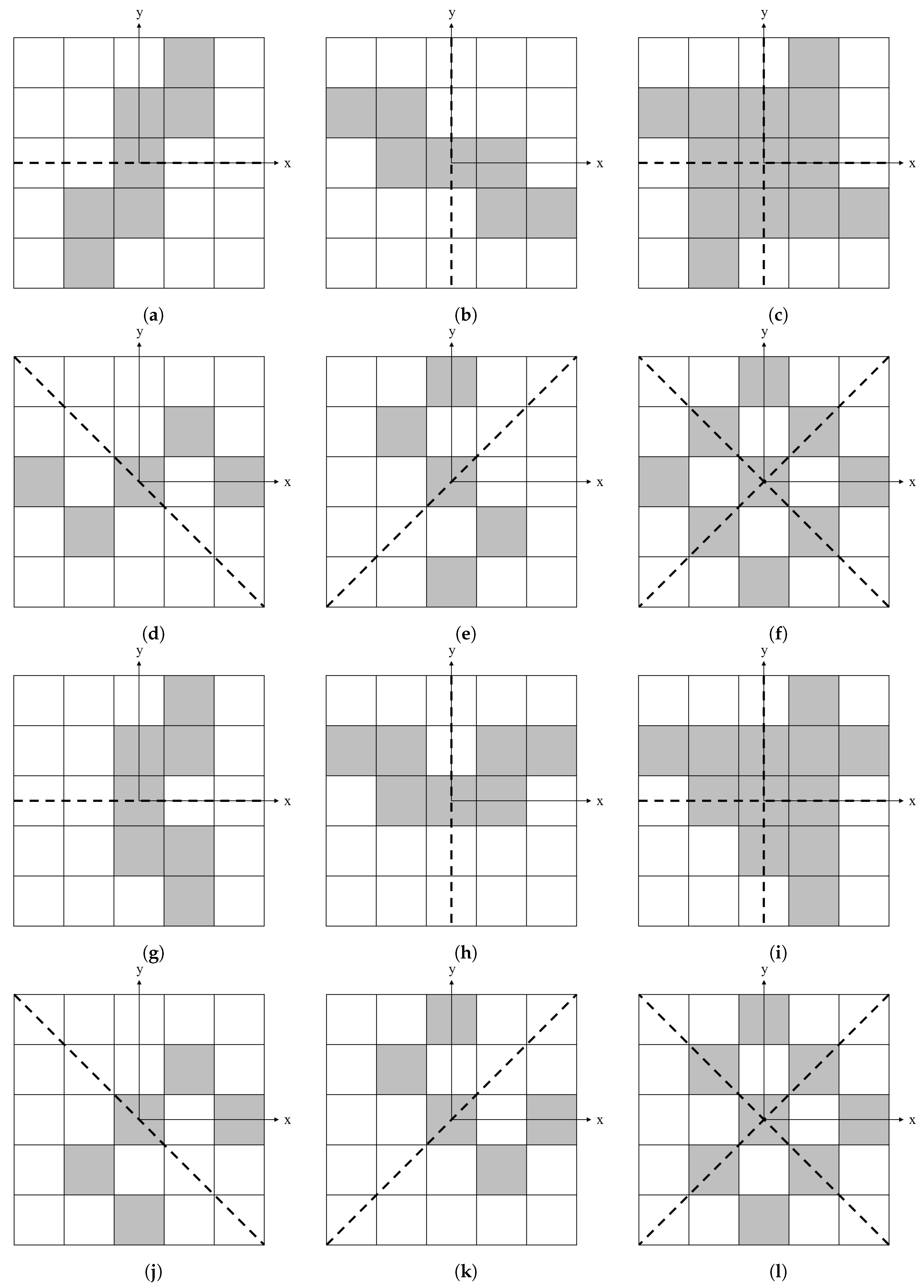
| Symmetry Axis | Rotational Axiom | Reflective Axiom |
|---|---|---|
| Horizontal | [F]++++[F] | [F]++++(F) |
| Vertical | − −[F]++++[F] | − −[F]++++(F) |
| Horizontal and vertical | [F]++[F]++[F]++[F] | [F]++(F)++[F]++(F) |
| Diagonal | +[F]++++[F] | +[F]++++(F) |
| Negative diagonal | −[F]++++[F] | −[F]++++(F) |
| Diagonal and negative diagonal | +[F]++[F]++[F]++[F] | +[F]++(F)++[F]++(F) |
| Parameter | Min | Max |
|---|---|---|
| Num Axioms | 1 | Number of predefined axioms |
| Number of rules | 1 | Total domain |
| Rule length | 2 | 5 |
| Number of iterations | 1 | 5 |
| Parameter | Min | Max |
|---|---|---|
| Num of Hidden layers | 2 | 10 |
| Size of first layer | 2 | 32 |
| Element removal threshold | 0 | 100 |
| Method | Function Evaluations | Standard Deviation |
|---|---|---|
| Random | 945 | 128 |
| L-System | 398 | 198 |
| CPPN | 650 | 54 |
Disclaimer/Publisher’s Note: The statements, opinions and data contained in all publications are solely those of the individual author(s) and contributor(s) and not of MDPI and/or the editor(s). MDPI and/or the editor(s) disclaim responsibility for any injury to people or property resulting from any ideas, methods, instructions or products referred to in the content. |
© 2023 by the authors. Licensee MDPI, Basel, Switzerland. This article is an open access article distributed under the terms and conditions of the Creative Commons Attribution (CC BY) license (https://creativecommons.org/licenses/by/4.0/).
Share and Cite
Venter, M.P.; Conradie, N.T. Intermediate Encoding Layers for the Generative Design of 2D Soft Robot Actuators: A Comparison of CPPN’s, L-Systems and Random Generation. Math. Comput. Appl. 2023, 28, 68. https://doi.org/10.3390/mca28030068
Venter MP, Conradie NT. Intermediate Encoding Layers for the Generative Design of 2D Soft Robot Actuators: A Comparison of CPPN’s, L-Systems and Random Generation. Mathematical and Computational Applications. 2023; 28(3):68. https://doi.org/10.3390/mca28030068
Chicago/Turabian StyleVenter, Martin Philip, and Naudé Thomas Conradie. 2023. "Intermediate Encoding Layers for the Generative Design of 2D Soft Robot Actuators: A Comparison of CPPN’s, L-Systems and Random Generation" Mathematical and Computational Applications 28, no. 3: 68. https://doi.org/10.3390/mca28030068