Evaluation of Physics-Informed Neural Network Solution Accuracy and Efficiency for Modeling Aortic Transvalvular Blood Flow

Abstract

Physics-Informed Neural Networks (PINNs) are a new class of machine learning algorithms that are capable of accurately solving complex partial differential equations (PDEs) without training data. By introducing a new methodology for fluid simulation, PINNs provide the opportunity to address challenges that were previously intractable, such as PDE problems that are ill-posed. PINNs can also solve parameterized problems in a parallel manner, which results in favorable scaling of the associated computational cost. The full potential of the application of PINNs to solving fluid dynamics problems is still unknown, as the method is still in early development: many issues remain to be addressed, such as the numerical stiffness of the training dynamics, the shortage of methods for simulating turbulent flows and the uncertainty surrounding what model hyperparameters perform best. In this paper, we investigated the accuracy and efficiency of PINNs for modeling aortic transvalvular blood flow in the laminar and turbulent regimes, using various techniques from the literature to improve the simulation accuracy of PINNs. Almost no work has been published, to date, on solving turbulent flows using PINNs without training data, as this regime has proved difficult. This paper aims to address this gap in the literature, by providing an illustrative example of such an application. The simulation results are discussed, and compared to results from the Finite Volume Method (FVM). It is shown that PINNs can closely match the FVM solution for laminar flow, with normalized maximum velocity and normalized maximum pressure errors as low as $5.74\%$ and $9.29\%$, respectively. The simulation of turbulent flow is shown to be a greater challenge, with normalized maximum velocity and normalized maximum pressure errors only as low as $41.8\%$ and $113\%$, respectively.

1. Introduction

Computational Fluid Dynamics (CFD) methods have become an essential tool in many engineering industries, from aerospace to biomedical. While traditional CFD methods, such as the Finite Volume Method (FVM), are proven and versatile tools, they have limitations, such as being ill-suited to solving ill-posed problems where the solution space is not fully confined by the boundary conditions alone. In heat transfer and biomedical applications, it is often difficult or impossible to determine exact boundary conditions for simulations; however, sparsely distributed measurement data are often readily available: the incorporation of these measurements could theoretically be used to constrain the solution, and to allow for the solution of the unknown boundary conditions. Unfortunately, this is a prohibitively expensive task to perform using traditional methods.

A further limitation of traditional CFD methods is the high computational expense of many-query-analysis type problems, such as simulation-based design, real-time monitoring using virtual sensors and model-predictive control: in these applications, the solution of a partial differential equation (PDE) is required for a large number of different boundary conditions or material properties. The computational expense can be partially alleviated by using surrogate models [1], but the construction of a data-fit surrogate model still requires a large dataset to be collected before the model can be constructed.

The physics informed neural network (PINN), first introduced by Raissi et al. [2], is an alternative fluid simulation and modeling technique that could potentially overcome the limitations mentioned above, and thus be a valuable tool in fluid dynamics research and modeling efforts. The PINN is a versatile, deep-learning-based modeling technique that allows for the solving of PDEs [3], the construction of surrogate models [4] and the solving of ill-posed problems [5].

With a PINN, a neural network is used as a general function approximator, and is trained to approximate the solution of a PDE. Typically, the training of a neural network requires a large amount of labeled training data: this requirement is lifted, by assembling a loss function that enforces known physics. Given that the problem is well-posed, the PINN method can be used to solve PDEs without any labeled data [3,4,6,7,8,9].

Currently, PINNs are more computationally expensive than traditional CFD techniques, when simulating a single, well-posed, unparameterized problem. However, when the dimensionality of the problem is increased (for example if we want to characterize the performance of an airfoil over a range of geometric parameters), the computational expense of PINNs scales favorably, due to the fact that PINNs can be trained on the entire parameter space simultaneously. Once a PINN has been trained, it can be used to rapidly infer solutions to the problem for any value of the parameter inside the training range. This makes PINNs promising candidates for use in system-level models, design optimization, real-time monitoring and control applications.

It has been shown by Sun et al. [4] that PINNs can be used to solve the Navier–Stokes Equations on a parameterized domain without labeled data: here, PINNs were presented as a method of constructing surrogate models in a data-sparse setting. The authors argued that in many scientific applications, large training datasets are not available, and that traditional data-fit surrogate models fail when the physical system exhibits strong nonlinearity. The authors constructed surrogate models for pipe flows with variable viscosity and laminar flow through a simplified artery with a variable degree of stenosis or aneurysm. The degree of stenosis or aneurysm was treated as a continuous parameter. They showed that PINNs can be used to solve the parameterized problem accurately without any labeled training data, and that the resulting surrogate model can be used to rapidly infer the flow field for any value of the geometry parameter inside the training range.

PINNs are also capable of solving multi-physics problems that have a greater number of transport equations that must be solved simultaneously. It was shown by Laubscher [9] that PINNs can accurately solve an incompressible, viscous flow problem with heat transfer and species diffusion. A dry air humidification problem was simulated, by using a mixed variable approach [10], which avoided higher-order derivatives in the governing equations. The author also introduced a segregated-network architecture that used three separate neural networks to approximate the energy equation, the species diffusion equation and the Navier–Stokes equations, respectively: this architecture was shown to be more accurate than the standard, single-network PINN architecture. A hyperparameter search was performed, to investigate the importance of the number of hidden layers, the number of neurons per layer and the number of sampling points in the domain. A parameterized version of the problem was also solved, to illustrate the potential of PINNs for surrogate modeling. The PINN performance was evaluated by comparing the results to a reference, finite volume method (FVM) solution.

In this paper, we attempted to use PINNs as a PDE integrator, meaning that we used PINNs to solve a well-posed problem without the use of any labeled training data: this is currently a challenging task for PINNs; there are, however, many examples in the literature where PINNs are used in novel ways that include the use of sparse training data [5,11,12,13,14].

In the field of biomedical engineering, patient-specific modeling is becoming an attainable and desirable practice; however, uncertainty in the boundary conditions of flow problems makes this a difficult task to perform using traditional CFD methods. Arzani et al. [14] showed how PINNs can be used to recover high-resolution wall shear stress estimates in aneurysms and stenoses, using sparse, noisy velocity measurements and unknown boundary conditions. Wall shear stress is a difficult quantity to measure in vivo, but it has been shown to play an important role in cardiovascular disease [15]. Arzani et al. used synthetic data, but the method could be applied to real patient-specific modeling, by using 4D flow magnetic resonance imaging (MRI) data to get noisy, low-resolution velocity measurements, and then using PINNs to recover high-resolution wall shear stresses.

Another area where boundary conditions are often unknown is heat transfer. Heat transfer problems are plagued by the difficulty of determining exact thermal boundary conditions. In most engineering applications, idealized boundary conditions are used for simulations, and in industry, engineers rely on experience to effectively operate equipment: PINNs offer a way to bridge this gap between real-world conditions and mathematical models. Cai et al. [5] used PINNs to simulate various heat transfer problems with complex, unknown boundary conditions, by using sparse, synthetic measurement data to constrain the solution. They illustrated the simulation of single-phase, multiphase, moving-boundary, steady, and unsteady flow problems. They also presented a method for using PINNs to inform sensor placement, to minimize the number of measurements required to accurately solve the problem.

The simulation of turbulent flow using PINNs for forward mode problems has proved to be a challenging task: different approaches have been used, including solving Reynolds-Averaged Navier-Stokes (RANS) equations with [16] and without [13], a turbulence closure model, and direct numerical simulation [17]. The Reynolds decomposition allows the simulation of turbulent flows at a lower computational cost, compared to direct numerical simulation; however, RANS turbulence closure models introduce assumptions and simplifications that make them less generalizable [18]. Eivazi et al. [13] showed that PINNs can be used to solve the RANS equations without any specific modeling assumptions or closure models, and by only using measurement data on the problem boundaries: this includes measurements of the Reynolds stresses that are difficult to measure in practice.

The PINN method is still in its infancy, and requires much further development. In this paper, we evaluated the use of Physics-Informed Neural Networks (PINNs) as an alternative method of simulating fluid flow through a simplified 2D aortic valve geometry, with the end goal of developing surrogate models.

A variety of techniques from the literature were implemented that have improved the training and prediction performance of PINNs [7,19,20]. Flow in the laminar and turbulent regimes were simulated by solving the incompressible Navier–Stokes and RANS equations, respectively. The results are compared to those obtained by using the Finite Volume Method (FVM), and are shown to be in good agreement. The PINN method is shown to be a promising candidate for use in system-level models, design optimization, real-time monitoring, control applications and inverse modeling.

2. Case Study Setup

To demonstrate the use of PINNs in simulating fluid flow, and to compare the results to those obtained by using the FVM, a simple example problem was chosen to be simulated: transvalvular blood flow through an aortic valve with various degrees of stenosis in the laminar and turbulent regimes.

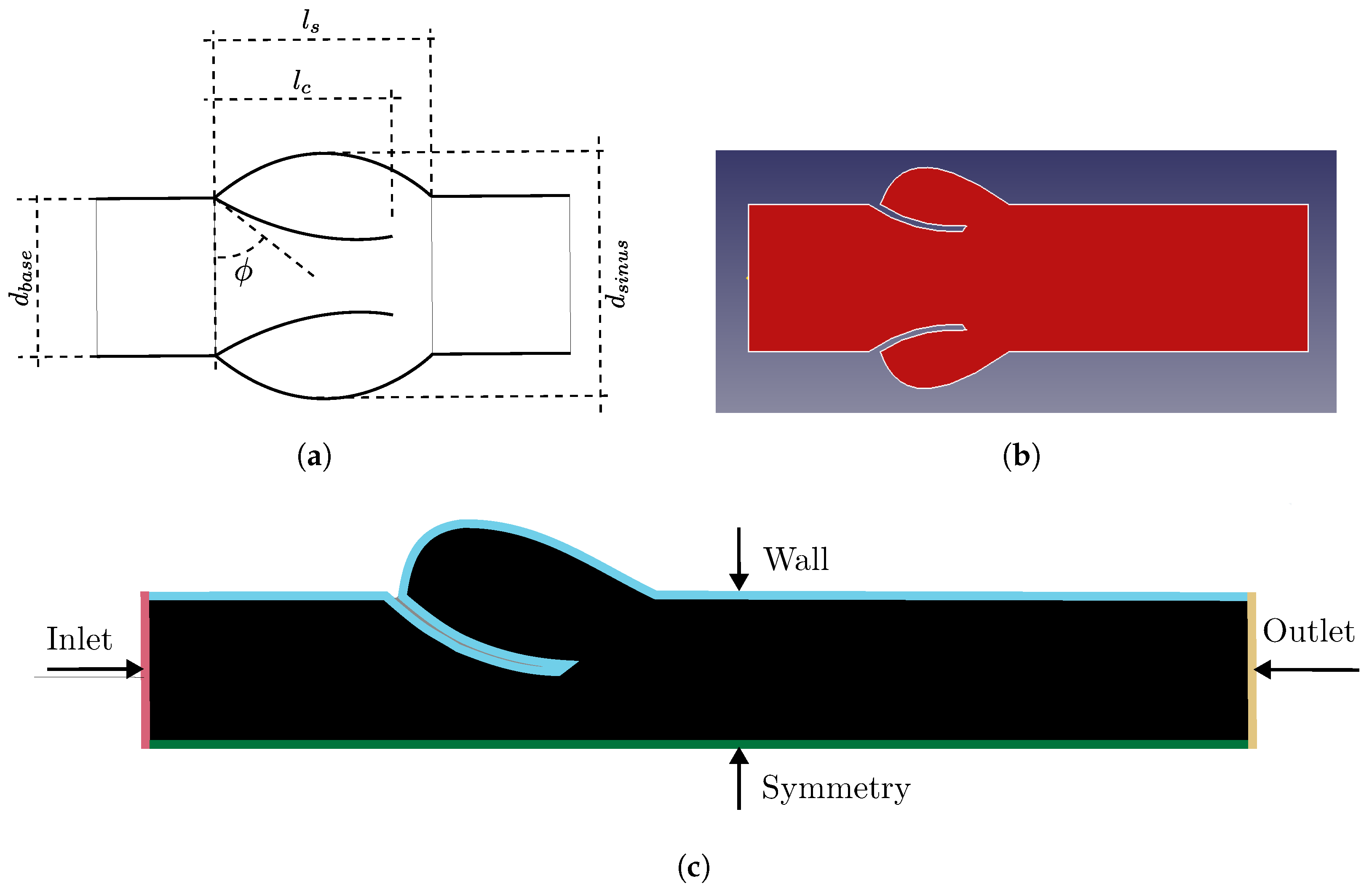
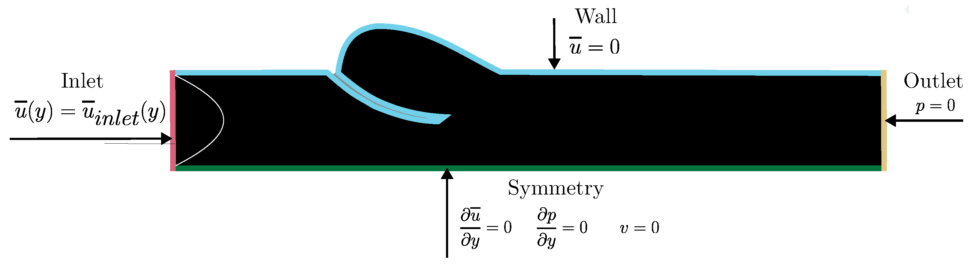
A simplified 2D geometry of an adult male aortic valve was used. As a result of the simlification, the solution was not necessarily an accurate approximation of real transvalvular blood flow: this was, however, not required, as the aim of the study was to discuss the application of PINNs to forward-mode fluid modeling, and to compare simulation results from the PINN method to the FVM method.

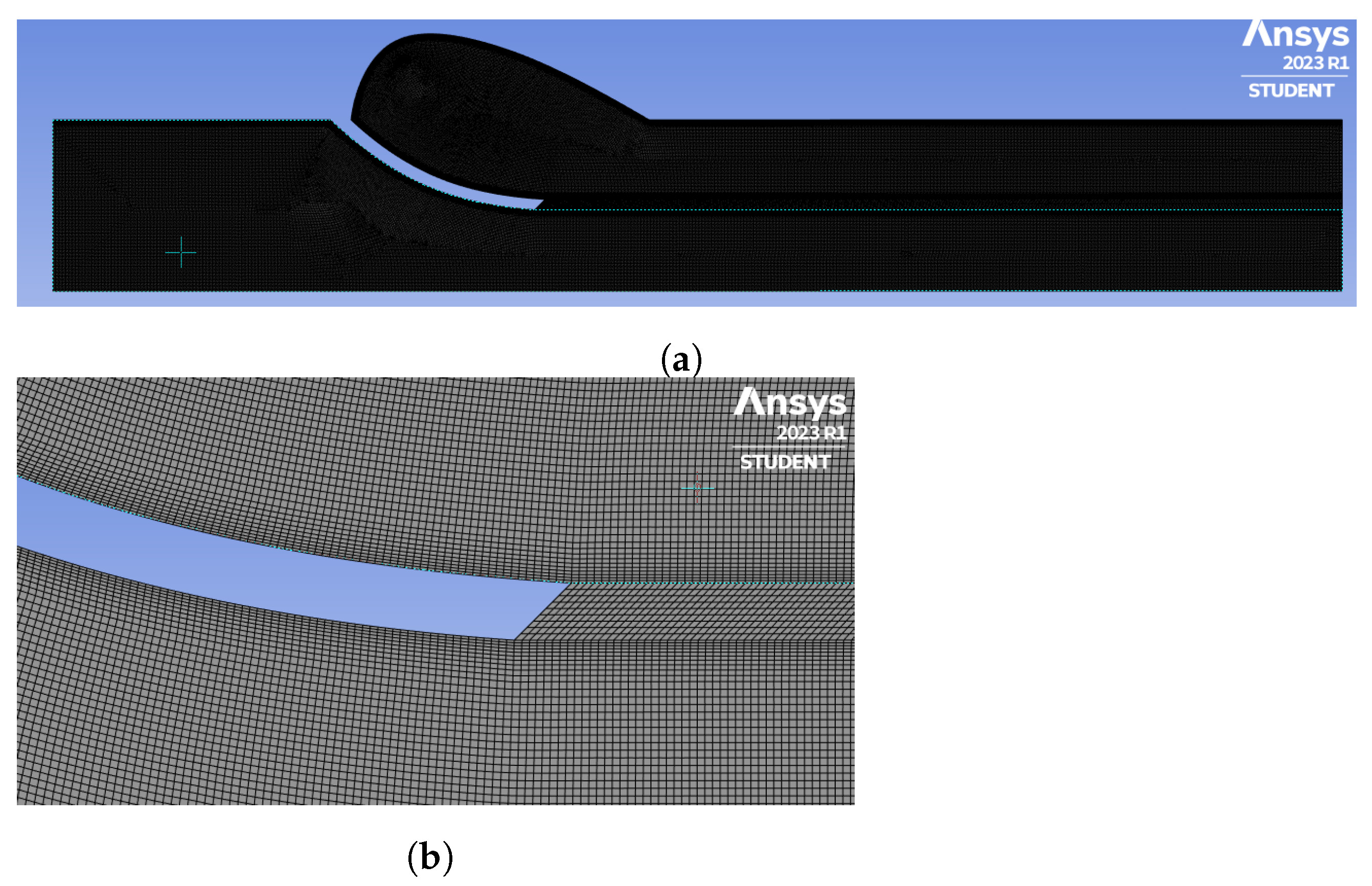
Figure 1 illustrates the computational domain used to represent a typical aortic valve. The inlet, outlet, wall and symmetry boundary conditions were imposed on the geometry, as shown in Figure 1c. The dimensions are tabulated in

Table 1. Aortic valve dimensions.

Parameter	Symbol	Value	Units	Reference
base diameter	$d_{base}$	24.7	[mm]	[21]
sinus diameter	$d_{sinus}$	36.1	[mm]	[22]
sinus length	$l_s$	21.5	[mm]	[22]
leaflet length	$l_c$	18.9	[mm]	[22]

.

Turbulent blood flow can be approximately described by the incompressible Reynolds-Averaged Navier–Stokes equations:

$$\begin{array}{cccc}\hfill \rho \frac{\partial \mathbf{u}}{\partial t}+\rho (\mathbf{u}·\nabla )\mathbf{u}& =-\nabla p+(\mu +{\mu }_t){\nabla }^2\mathbf{u}+\mathbf{f}\hfill & \hfill & \mathbf{x},t\in {\Omega }_{f,t},\mathit{\theta }\in \mathbb{R}\hfill \end{array}$$

(1)

$$\begin{array}{cccc}\hfill \nabla ·\mathbf{u}& =0\hfill & \hfill & \mathbf{x},t\in {\Omega }_{f,t},\mathit{\theta }\in \mathbb{R}\hfill \end{array}$$

(2)

where $\mathbf{x}\mathrm{and}t$ are dimensions of space and time, ${\Omega }_{f,t}\in \mathbb{R}$ is the problem domain in space and time, $\mathit{\theta }$ is a vector of fluid properties—such as $\rho$: density and $\mu$: viscosity—and ${\mu }_t$ is the turbulent viscosity. Given suitable boundary and initial conditions, the solution for the mean velocity field, $\mathbf{u}$, and the mean pressure field, p, is uniquely defined.

Here, we approximated the fluid to have a linear-strain-rate–stress relationship, with a dynamic viscosity of 0.004 Pa·s: this was accurate at the high Reynolds numbers that the transvalvular flow was expected to have [23]. A density of 1055 kg/m³ was used [24].

A turbulence closure model was required, to compute the turbulent viscosity. A mixing length model [18] was chosen for the PINN and the FVM simulations. Mixing length models have a very narrow range of applicability in modern CFD, as they are incapable of accurately representing flows that include recirculation or flow separation [18]. Modern CFD routinely uses turbulence models, such as the $k-ϵ$ and $k-\omega$ models, which are much more appropriate for general flows; however, the current state of the art in data-less PINNs does not yet allow for the inclusion of these models, as they increase the stiffness of the system of equations to be solved.

The mixing length model was an algebraic model, which means that the turbulent viscosity was directly computed from the mean velocity field, without solving an additional set of equations. The turbulent viscosity was computed as follows:

$$\begin{array}{cc}\hfill {\mu }_t\left(\mathbf{x}\right)& =\rho {\left(l_m\left(\mathbf{x}\right)\right)}^2\sqrt{G\left(\mathbf{x}\right)}\hfill \end{array}$$

(3)

$$\begin{array}{cc}\hfill G\left(\mathbf{x}\right)& =2{\left(\frac{\partial u}{\partial x}\left(\mathbf{x}\right)\right)}^2+2{\left(\frac{\partial v}{\partial y}\left(\mathbf{x}\right)\right)}^2+{\left(\frac{\partial u}{\partial y}\left(\mathbf{x}\right)+\frac{\partial v}{\partial x}\left(\mathbf{x}\right)\right)}^2\hfill \end{array}$$

(4)

where $l_m$ was the mixing length, and G was the strain-rate tensor. Various formulations can be used to compute an appropriate mixing length. The formulation used in this work is discussed later.

To simulate a laminar case, the governing equation was the same as the turbulent case, as shown in Equation (1), but the turbulent viscosity was simply set to zero.

Various degrees of stenosis were considered, by setting the valve leaflets to different angles, which restricted the flow by different degrees as shown in

Table 2. Degrees of stenosis.

Valve Angle	Area Ratio	Degree of Stenosis
35	0.113	Very Severe
45	0.227	Severe
55	0.395	Moderate
75	0.808	None

. The area ratio was defined as the ratio of the area of the smallest restriction in the valve to the area of the base.

This study did not include a comparison of simulation results to clinical data. The aim of this study was not to simulate a realistic case, but to compare the PINN method to the FVM method. As a simplified geometry was used, the results were not expected to be an accurate representation of real transvalvular blood flow.

3. Physics-Informed Neural Networks

With the PINN method, first proposed by Raissi et al. [2], we aimed to solve the PDE problem in a fundamentally different way than with the FVM.

Traditionally, the PDE problem has been solved by discretizing the PDE, and solving the resulting system of equations.

The PINN method aims to solve the PDE problem by constraining and training a neural network to satisfy any symmetries, conservation principles, invariances or boundary conditions that are known to hold for the system.

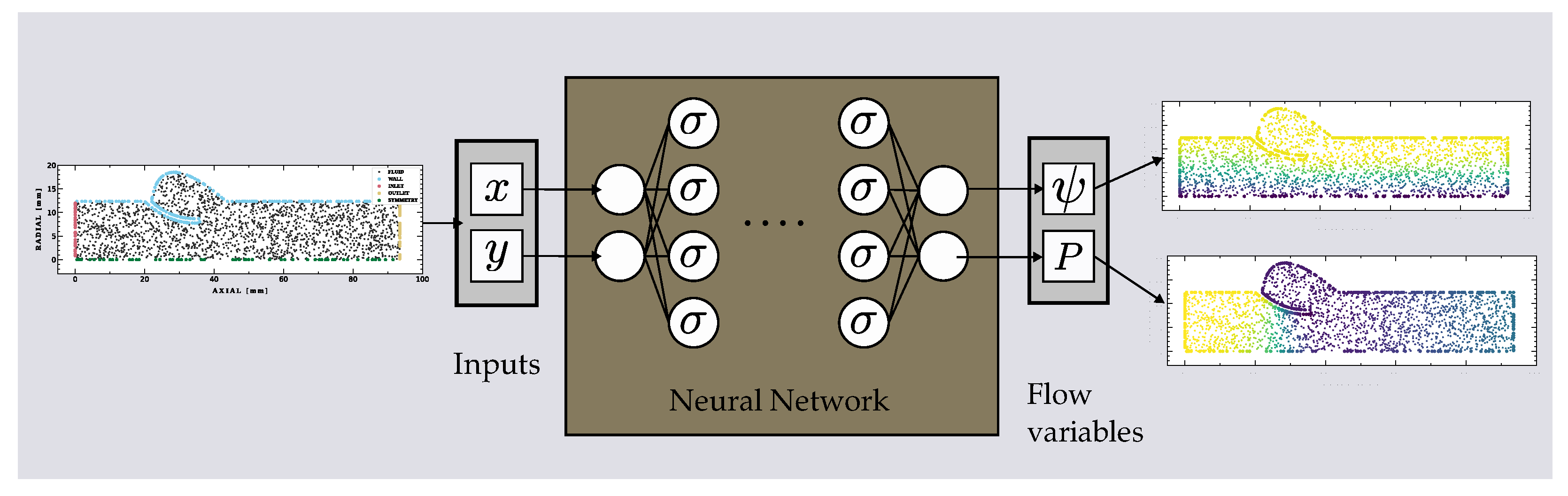
After training, what we are left with is a neural network that can infer the solution of the PDE at any point in the domain, as shown in Figure 2. An attractive property of this solution is that it is continuous in the domain, and that inference is very fast once the model has been trained: this makes PINNs valuable surrogate modeling tools.

3.1. Problem Formulation

In this paper, the stream function pressure formulation was used as the preferred formulation of the Navier–Stokes equations. We defined the scalar stream function $\psi$, such that

$$u=\frac{\partial \psi }{\partial y}\mathrm{and}v=-\frac{\partial \psi }{\partial x}$$

(5)

was true. Equations (5) were substituted into the Navier–Stokes Equations (1) and (2), to obtain the stream function pressure formulation.

This formulation was preferred, as it automatically satisfied mass conservation: this came at the computational cost of having to calculate third-order derivatives in diffusion terms.

For this case study, velocity results differed by several orders of magnitude from pressure results. This caused an imbalance in the loss function, which had larger terms associated with pressure, and smaller terms associated with the velocities. This imbalance was severely detrimental to the optimization process, and could cause the model training to fail outright. To remedy this, the governing equations were non-dimensionalized. The non-dimensional variables were defined as:

$$\begin{array}{c}\hfill x^{*}=\frac{x}{l_c},y^{*}=\frac{y}{l_c},\end{array}$$

(6)

$$\begin{array}{c}\hfill u^{*}=\frac{u}{u_c},v^{*}=\frac{v}{u_c},p^{*}=\frac{p}{\rho u_c^2}\end{array}$$

(7)

where the characteristic length $l_c$ was the diameter of the base, and the characteristic velocity $u_c$ was the inlet velocity. The non-dimensionalized stream function can be written as:

$${\psi }^{*}=\frac{\psi }{u_c{l}_c}$$

(8)

3.2. Mathematical Description of the PINN

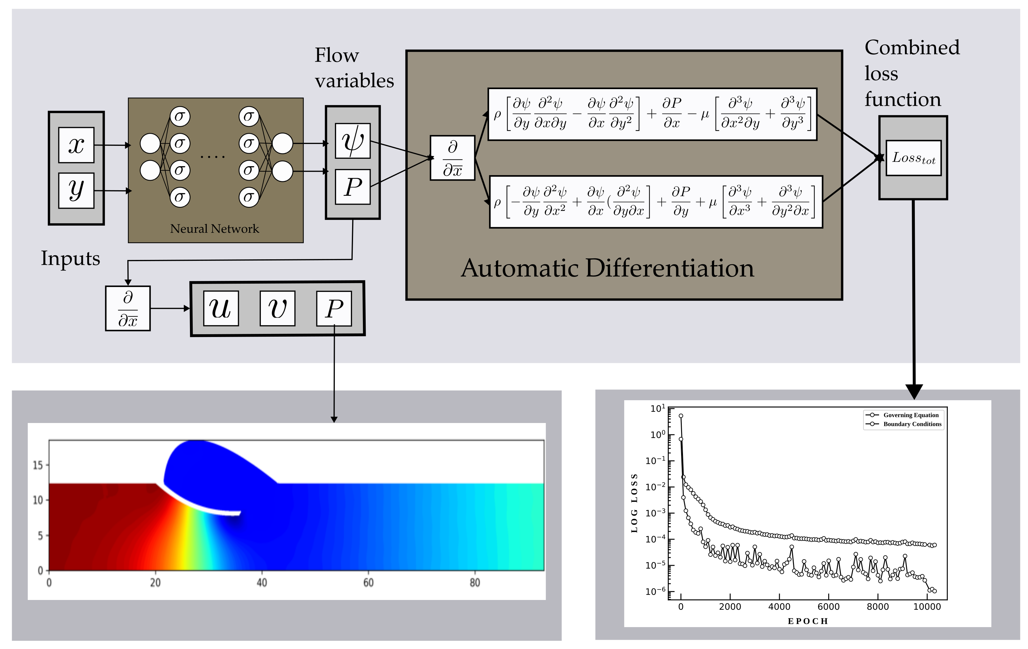
The PINN method uses a neural network as a flexible mathematical function that can be used to represent an approximate solution to a given PDE problem; however, the PINN method differs from typical regression methods, in that the neural network is not trained in a supervised manner, to approximate a function. Instead, we treat the network as a function that must satisfy all the invariances, symmetries and boundary conditions that are known to hold for the physical system. If the invariances, symmetries and boundary conditions are indeed consistent, the solution is unique, and the loss function will have a minimum that corresponds to the solution of the PDE problem, which can be found using a nonlinear optimizer. An overview of the PINN method is shown in Figure 3.

In the subsequent section, we will elaborate on the derivation of the loss function, which constitutes a crucial distinction between Physics-Informed Neural Networks and conventional neural networks. By encoding the known physics of the system, the PINN loss function facilitates training without labeled data.

As shown in Figure 3, the PINN architecture contains a fully connected neural network (NN) that is attached to a training section. The NN is expressed mathematically as a nonlinear operator $:\mathcal{N}$

$$\zeta \left(\mathbf{x}\right)=\mathcal{N}(\mathbf{x},\mathbf{w})$$

(9)

where $\mathbf{x}\in {\mathbb{R}}^{n\times d}$ is a matrix of n samples in Cartesian coordinates, each with dimensionality $d=2$; $\mathbf{w}\in {\mathbb{R}}^q$ is the vector of q model parameters; and $\zeta \in {\mathbb{R}}^{n\times m}$ is a matrix of $m=2$ predicted flow variables.

$$\begin{array}{ccc}\hfill \mathbf{x}=\left[\begin{array}{c}{x}^{*}\\ y^{*}\end{array}\right]& \hfill & \hfill \zeta =\left[\begin{array}{c}{\psi }^{*}\\ p^{*}\end{array}\right]\end{array}$$

(10)

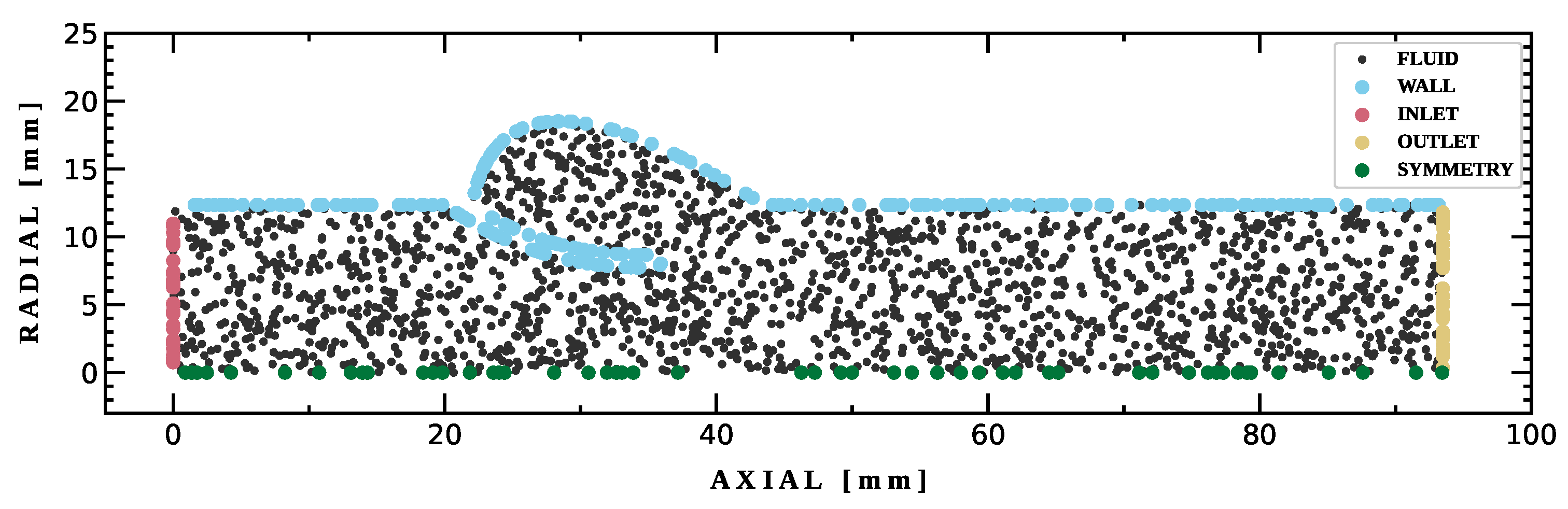
To train the NN, a composite loss function, $\mathcal{L}$, is assembled and evaluated at several pseudo-randomly spaced locations in the domain during each training iteration. These sample locations are called collocation points, and are shown in Figure 4.

Collocation points are generated using the FreeCAD software package [25], which offers great flexibility via the python API, is free and is open source. Points are placed in the domain, and are pseudo-randomly distributed according to a Sobol sequence. The Sobol sequence offers a good compromise between uniformity and low discrepancy in the placement of collocation points [26].

The loss function is composed of multiple terms, with each term corresponding to a conservation law, boundary condition or other constraints, enforced using the penalty method, which penalizes deviation of the network output from the constraints in a soft manner (soft constraints are never perfectly satisfied as opposed to hard constraints that are. As the loss function is minimized, soft constraints get closer to being satisfied, but a residual always remains). The loss function is written as:

$$\mathcal{L}\left(\mathbf{w}\right)=\lambda \frac{1}{n}\sum _{i=1}^n{\left(f_j\left({\mathbf{x}}_{\mathbf{i}}\right)\right)}^2$$

(11)

where $\lambda \in {\mathbb{R}}^j$ is a vector of j manually tuned weights, $f_j$ is the $j^{{}^{\prime }}$th residual function, and $n_j$ is the number of collocation points where $f_j$ is evaluated.

The residual functions to be minimized are the governing equations: namely, the momentum conservation equations and the boundary conditions. Mathematically, they are expressed as:

Governing Equations: Momentum Conservation:

$$\begin{array}{ccc}& f_{mom;x}\left(\mathbf{x}\right)=\left[\frac{\partial {\psi }^{*}}{\partial y^{*}}\left(\mathbf{x}\right)\frac{{\partial }^2{\psi }^{*}}{\partial x^{*}\partial y^{*}}\left(\mathbf{x}\right)-\frac{\partial {\psi }^{*}}{\partial x^{*}}\left(\mathbf{x}\right)\frac{{\partial }^2{\psi }^{*}}{\partial y^{*2}}\left(\mathbf{x}\right)\right]+\frac{\partial p^{*}}{\partial x^{*}}\left(\mathbf{x}\right)\hfill & \\ & -\frac{(\mu +{\mu }_t\left(\mathbf{x}\right))}{\rho u_c{l}_c}\left[\frac{{\partial }^3{\psi }^{*}}{\partial x^{*2}\partial y^{*}}\left(\mathbf{x}\right)+\frac{{\partial }^3{\psi }^{*}}{\partial y^{*3}}\left(\mathbf{x}\right)\right]\approx 0\mathbf{x}\in {\Gamma }_{fluid}\hfill \end{array}$$

(12)

$$\begin{array}{cccc}& f_{mom;y}\left(\mathbf{x}\right)=\left[-\frac{\partial {\psi }^{*}}{\partial y^{*}}\left(\mathbf{x}\right)\frac{{\partial }^2{\psi }^{*}}{\partial x^{*2}}\left(\mathbf{x}\right)+\frac{\partial {\psi }^{*}}{\partial x^{*}}\left(\mathbf{x}\right)\frac{{\partial }^2{\psi }^{*}}{\partial y^{*}\partial x^{*}}\left(\mathbf{x}\right)\right]+\frac{\partial p^{*}}{\partial y^{*}}\left(\mathbf{x}\right)\hfill & & \\ & +\frac{(\mu +{\mu }_t\left(\mathbf{x}\right))}{\rho u_c{l}_c}\left[\frac{{\partial }^3{\psi }^{*}}{\partial x^{*3}}\left(\mathbf{x}\right)+\frac{{\partial }^3{\psi }^{*}}{\partial y^{*2}\partial x^{*}}\left(\mathbf{x}\right)\right]\approx 0\mathbf{x}\in {\Gamma }_{fluid}\hfill & \end{array}$$

(13)

Boundary Conditions: no slip wall:

$$f_{wall}\left(\mathbf{x}\right)=\overline{u^{*}}\left(\mathbf{x}\right)\approx 0 \mathbf{x}\in {\Gamma }_{wall}$$

(14)

Boundary Conditions: specified velocity inlet:

$$f_{inlet}\left(\mathbf{x}\right)=\overline{u^{*}}\left(\mathbf{x}\right)-{\overline{u^{*}}}_{inlet}\left(\mathbf{x}\right)\approx 0 \mathbf{x}\in {\Gamma }_{inlet}$$

(15)

Boundary Conditions: reference pressure outlet:

$$f_{outlet}\left(\mathbf{x}\right)=p^{*}\left(\mathbf{x}\right)-p_{outlet}^{*}\left(\mathbf{x}\right)\approx 0 \mathbf{x}\in {\Gamma }_{outlet}$$

(16)

Boundary Conditions: symmetry plane:

$$f_{sym;1}\left(\mathbf{x}\right)=\frac{\partial p^{*}}{\partial \overline{n}}\left(\mathbf{x}\right)\approx 0 \mathbf{x}\in {\Gamma }_{symmetry}$$

(17)

$$f_{sym;2}\left(\mathbf{x}\right)=\frac{\partial \overline{u^{*}}}{\partial \overline{n}}\left(\mathbf{x}\right)\approx 0 \mathbf{x}\in {\Gamma }_{symmetry}$$

(18)

$$f_{sym;3}\left(\mathbf{x}\right)=\overline{u^{*}}\left(\mathbf{x}\right)·\overline{n}\approx 0 \mathbf{x}\in {\Gamma }_{symmetry}$$

(19)

where $\overline{u^{*}}$ is the dimensionless velocity vector, ${\overline{u^{*}}}_{inlet}$ is the dimensionless prescribed inlet velocity, $p^{*}$ is the dimensionless pressure, $p_{outlet}^{*}$ is the dimensionless reference outlet pressure, $\overline{n}$ is the boundary normal vector, and ${\Gamma }_{wall}$, ${\Gamma }_{inlet}$, ${\Gamma }_{outlet}$, and ${\Gamma }_{symmetry}$ are the wall, inlet, outlet and symmetry boundary domains, respectively.

To evaluate the loss function, derivatives of the network outputs are required, as can be seen by the derivative terms in the equations above. These derivatives are computed using automatic differentiation, which allows the computation of the gradients of $\mathcal{N}$ with respect to $\mathbf{x}$, as $\mathcal{N}$ is a computational graph. Interested readers are directed to Güene et al. [27] for a detailed explanation of automatic differentiation, and how it differs from numerical differentiation.

3.3. Training

Once the loss function $\mathcal{L}$ is defined, a solution can be computed, by applying a stochastic gradient descent algorithm, such as ADAM [28], to find the values of the network weights that minimize $\mathcal{L}$.

At each iteration of the training algorithm, a mini-batch of collocation points is sampled from the domain, and the loss function is evaluated. ADAM is a gradient-based optimization algorithm, which means that derivatives of the loss function must also be computed: this is done efficiently, using automatic differentiation. The network weights are updated iteratively, for a fixed number of iterations.

Mini-batch subsampling is done, to enable the use of a larger set of collocation points, while still being able to take advantage of a Graphical Processing Unit (GPU) (an Nvidia GTX 1050Ti GPU was used for training), which has a limited amount of memory for training. Full batch training is done for the boundary conditions.

Convergence to a global minimum of the loss function is not guaranteed, and the algorithm will most likely converge to a local minimum. This is an inherent limitation of machine learning methods that rely on the formulation of a non-convex loss function and nonlinear optimizer. The result is some variability in the convergence speed and the final solution of each training run. In the authors’ experience, however, this variability is not significant enough to impact the practical usability of the method.

While the PINN training procedure does have inherent flaws, such as convergence to local minima, it also has inherent advantages, such as allowing the flexibility to incorporate measurement data into the solution, and the ability to solve parameterized problems in parallel.

3.4. Pinn Turbulence Model Implementation

The mixing length model, proposed by Hennning et al. for use in Nvidia Symnet [16], was chosen to compute the turbulent viscosity. To the authors’ knowledge, there are no publications that have used a more complex turbulence model with PINNs trained without labeled training data.

The turbulent viscosity was computed as explained in Section 2, with a mixing length [16] defined as:

$$l_m\left(\mathbf{x}\right)=min(0.419d\left(\mathbf{x}\right),0.09d_{max})$$

(20)

where wall distance d and maximum wall distance $d_{max}$ had to be efficiently computed. Commercial CFD solvers compute the normal wall distance efficiently by solving specially formulated PDEs, such as the Eikonal equations [29], in the same computational domain. We followed a similar approach, by solving a Poisson-type equation, as proposed by Spalding [30]:

$$\begin{array}{cc}\hfill {\nabla }^{2}L& =C\hfill \end{array}$$

(21)

$$\begin{array}{cc}\hfill d& =\pm \sqrt{\sum _{i=1,2}^{}{\left(\frac{\partial L}{\partial x_i}\right)}^2}+\sqrt{\sum _{i=1,2}^{}{\left(\frac{\partial L}{\partial x_i}\right)}^2+2L}\hfill \end{array}$$

(22)

with boundary conditions

$$\begin{array}{cc}\hfill L& =0\mathrm{on}{\Gamma }_{wall}\hfill \\ \hfill \frac{\partial L}{\partial \overline{n}}& =0\mathrm{on}{\Gamma }_{inlet},{\Gamma }_{outlet},{\Gamma }_{symmetry}\hfill \end{array}$$

where $x_i$ was the $i$th spatial dimension, $C=-1$, d was the wall distance, L was the level set function, and $\overline{n}$ was the boundary normal vector.

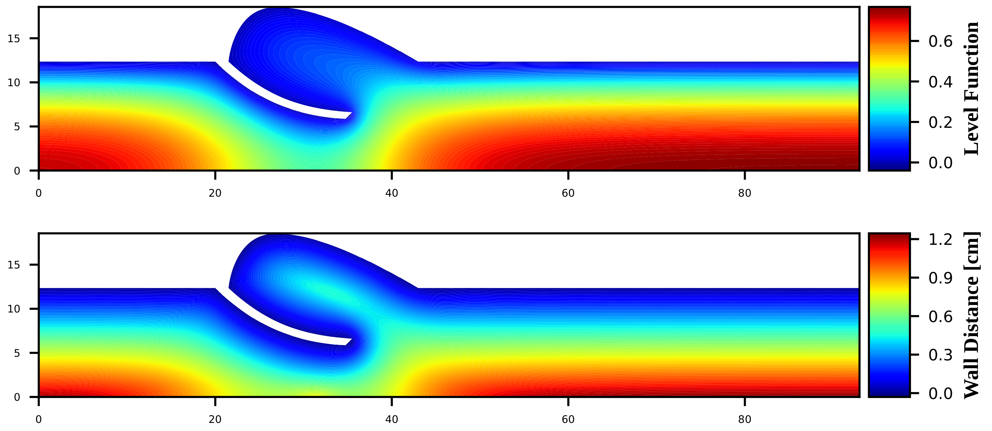
A separate PINN was used to solve Equation (21), and to recover the level set function L. As the PINN was differentiable by using automatic differentiation, the derivative terms $\frac{\partial L}{\partial x_i}$ and wall distance d could be efficiently computed using Equation (22). The level set function and wall distance are shown in Figure 5. Once the wall distance PINN was trained, it could be efficiently used to infer the wall distance at any point in the domain. As the geometry was static for each simulation case, the wall distance PINN only needed to be trained and evaluated once.

This is also a powerful approach to use when the geometry is dynamic. For example, in the case of a variable valve angle, the wall distance PINN can be trained to compute the wall distance for a continuous range of valve angles. Once the PINN is trained, it can rapidly infer the wall distance at any location, for any valve angle in that range.

The Poisson method yields a slightly less accurate wall distance, compared to the Eikonal method: this difference is, however, mostly in the region far from the wall, where it has little or no impact on the mixing length. The authors found that the Poisson method was sufficient for their purposes, and was easier to implement.

3.5. Gradient Enhanced PINN

To improve solution accuracy, we implemented a gradient-enhanced loss function, as proposed by Yu et al. [19]. This method was based on the observation that if we enforced a zero loss function across the entire domain, then the gradient of the loss function w.r.t the spatial dimensions would also need to be zero. We thus utilized the availability of gradient information, to add a loss term that penalized a non-zero gradient of the momentum residual functions, as shown in Equation (23):

$$\begin{array}{ccccc}\hfill {\mathcal{L}}_g\left(\mathbf{w}\right)={\lambda }_g\frac{1}{n}\sum _{i=1}^n{\left(\frac{\partial f_j}{\partial x_d}\left({\mathbf{x}}_{\mathbf{i}}\right)\right)}^2,& \hfill & \hfill \mathrm{where}& \hfill & \hfill j\in \{\mathrm{momentum}\mathrm{x},\mathrm{momentum}\mathrm{y}\}.\end{array}$$

(23)

The final loss function thus contained two terms that penalized deviation from momentum conservation in the x and y directions, and two additional terms that penalized the non-zero gradients of the first two terms in the x and y directions.

3.6. Fourier Layer

PINNs exhibit stiff training dynamics, which limit their practical use as a PDE solver. Many papers have focused on alternative network architectures, to enable faster training and more accurate solutions. In this paper, the Fourier layer, as proposed by Wang et al. [20], was implemented. Wang et al. [20] showed that PINNs are biased towards training low spatial frequencies in the solution faster than high frequencies. The Fourier layer aims to alleviate this spectral bias, by mapping the input coordinates to randomized sinusoidal features, before entering the network. The notation of Wang et al. [20], and the formulation of Tancik et al. [31],

$$\gamma \left(\mathbf{x}\right)=\left[\begin{array}{c}sin\left(\mathbf{B}\mathbf{x}\right)\\ cos\left(\mathbf{B}\mathbf{x}\right)\end{array}\right]$$

(24)

where $\mathbf{B}\in {\mathbb{R}}^{n\times d}$ is a random matrix, were used, with entries sampled from a Gaussian distribution with standard deviation $\sigma$. The standard deviation was a tunable parameter that changed the frequency of the spectral bias.

3.7. Skip Connections

A well-known phenomenon that complicates the training of deep neural networks is that of disappearing gradients. As the layer count increases, the gradients of the loss function, w.r.t model parameters, get smaller and smaller. This is also the case for gradients of the predicted flow variables, w.r.t input coordinates, which are used in the PINN loss function [7]. The decreasing strength of spatial derivative information leads to longer training times and less accurate solutions.

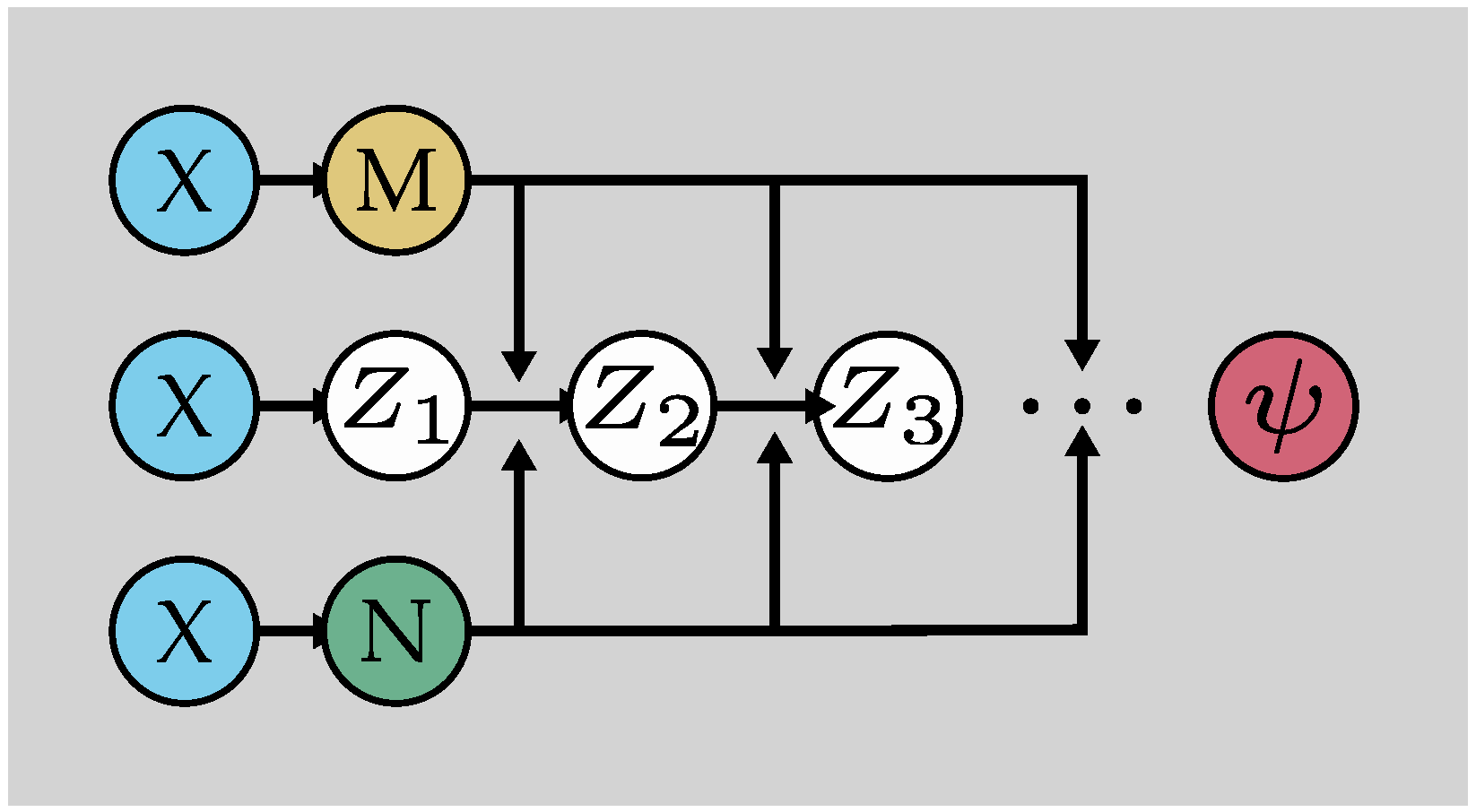
Shi, Liu and Huo [7] proposed a solution to this problem, by re-introducing spatial coordinate information into each layer of the network, as shown in Figure 6.

The forward propagation rule for the network at the $i$th layer is written as:

$$\begin{array}{cc}\hfill Z^i& =\sigma (W^i{Z}^{i-1}+b^i)·M+N\hfill \\ \hfill M& =\sigma (W_{M}X+b_M)\hfill \\ \hfill N& =\sigma (W_{N}X+b_N)\hfill \end{array}$$

(25)

where $Z^i$ is the output of the $i$th layer with weights $W^i$ and biases $b^i$, X is the input coordinates and $\sigma$ is the activation function. $W_M$ and $W_N$ are the weights of the M and N layers, respectively, while $b_M$ and $b_N$ are the biases of the M and N layers, respectively.

This method synergizes well with the gradient-enhanced PINN (gPINN) [19]. The additional gPINN loss function term, along with the $\psi -p$ formulation, results in fourth-order spatial gradients in the loss function: this makes this formulation especially sensitive to weak spatial gradients during training.

4. Fvm Reference Solution

As a reference solution, the problem was solved using the Ansys® 2023 R1 software suite. Mesh generation was done using Ansys Mechanical^® 2023 R1 [32], as shown in Figure 7: this resulted in a mixed quadrilateral and triangular element mesh with around 135,000 linear elements. Mesh inflation was used for 10 elements around the wall, to ensure good-quality elements around the wall, which were also aligned with the boundary. The meshing operation was performed using an intel i7 7700HQ processor.

The mesh was imported into Ansys Fluent^® 2023 R1 [33], to solve both the laminar and the turbulent cases. The same hardware was used for the solver as was used for the meshing operation. Boundary conditions were imposed, as shown in Figure 8. A specified velocity profile inlet condition, reference pressure of 0 Pa outlet condition, no-slip wall and symmetry plane were imposed.

4.1. Turbulence Modeling

For the turbulent solution, a mixing length turbulence model [18] was used. As mentioned before, this algebraic turbulence model does not have a transport equation for any turbulence properties, and thus requires no additional boundary conditions to be imposed beyond the laminar case.

The turbulent viscosity was calculated using a wall distance $l_m$ and shear rate G, as shown previously in Equation (3).

The official ANSYS Fluent^® user guide [34] does not disclose the exact method used to calculate the mixing length, $l_m$; however, the authors determined empirically that the mixing length was calculated using the same equation as the one used for the PINN formulation shown in Equation (3).

4.2. Equation Discretization and Solution

Similar discretization schemes were chosen for the laminar and turbulent solutions. The gradient terms were computed using a least-squares-based method. The face pressures were computed using a second-order (or central differencing) scheme. The divergence terms in the momentum equations were computed using a second-order upwind scheme [35].

The laminar solution was computed using a coupled solver, and the turbulent solution was computed using a SIMPLE solver [35].

The solution process was initialized by first computing the inviscid solution, and using the resulting velocity field as an initial guess for the viscous solution. The solution was then iterated until convergence was reached.

The convergence criteria for the viscous solution was a maximum absolute change in the area-averaged inlet pressure of ${10}^{-2}$ Pa: it was observed that if this criterion was met, the momentum and continuity residuals were also below ${10}^{-4}$.

5. Results

The metrics used to evaluate the accuracy of the PINN solution are expressed in Equations (26)–(29).

The first compares the peak jet velocities on the symmetry plane; the difference was normalized by the peak jet velocity of the FVM solution:

$$\begin{array}{cccc}\hfill e_1& =\frac{{\left(u_{max}\right)}_{PINN}-{\left(u_{max}\right)}_{FVM}}{{\left(u_{max}\right)}_{FVM}}·100u_{max}=\underset{i}{max}\left(\right||{\mathbf{u}}_{symmetry}^i{\left|\right|}_2)\hfill & & \hfill \end{array}$$

(26)

The second compares the transvalvular pressure drop: this was computed as the area-averaged pressure difference between the inlet and outlet; the difference was normalized by the transvalvular pressure drop of the FVM solution:

$$\begin{array}{ccc}\hfill e_2& =\frac{{\left(p_{drop}\right)}_{PINN}-{\left(p_{drop}\right)}_{FVM}}{{\left(p_{drop}\right)}_{FVM}}·100p_{drop}=\frac{1}{NA}\sum _{i=0}^N\left(A^i{p}_{inlet}^i\right)-p_{outlet}\hfill & \end{array}$$

(27)

The third is the maximum absolute error of the velocity magnitude, normalized by the maximum velocity magnitude of the FVM solution:

$$\begin{array}{cccc}\hfill e_3& =\frac{\left|\right|{\mathbf{u}}_{PINN}^i-{\mathbf{u}}_{FVM}^i{\left|\right|}_{\infty }^2}{{\left({\mathbf{u}}_{max}\right)}_{FVM}}·100\hfill & & \hfill \end{array}$$

(28)

The fourth is the maximum absolute error of the pressure field, normalized by the transvalvular pressure drop of the FVM solution:

$$\begin{array}{cccc}\hfill e_4& =\underset{i}{max}\left(\frac{|p_{PINN}^i-p_{FVM}^i|}{{\left(p_{drop}\right)}_{FVM}}\right)·100\hfill & & \hfill \end{array}$$

(29)

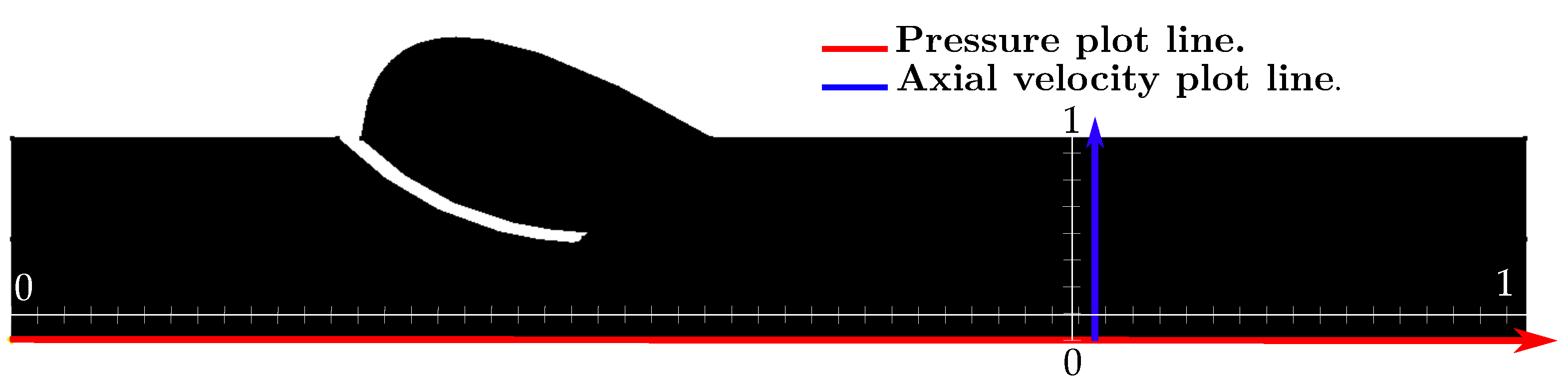
The solutions are also plotted along two lines intersecting the geometry, as shown in Figure 9.

The pressure is plotted on the first line, which runs along the symmetry plane: this illustrates the pressure change in the flow direction, as shown in Figures 11 and 13, in black.

The second line is perpendicular to the flow direction, just downstream of the valve: this is used to compare the axial velocity profile in the jet, as shown in Figures 11 and 13, in red.

5.1. Laminar Flow

Flow in the laminar regime was simulated for a range of valve angles between ${75}^{\circ }$ and ${35}^{\circ }$. A parabolic inlet velocity profile was used, with a volumetric flow rate of 46 mL/s: at this volume flow rate, the Reynolds number, based on the base diameter, was $Re=651$.

A four-layer neural network was used, with 20 neurons per layer, except for the Fourier encoding layer, which had 40 neurons. The network was trained for 5000 epochs, using the ADAM optimizer with a mini-batch size of 1024 and a collocation number count of 8727 for momentum conservation and 765 on all the boundaries combined. A learning rate of 1 × 10${}^{-3}$ was used (interested readers are referred to the classic text by Rao [36] for more background information on general mathematical optimization and the ADAM optimizer.).

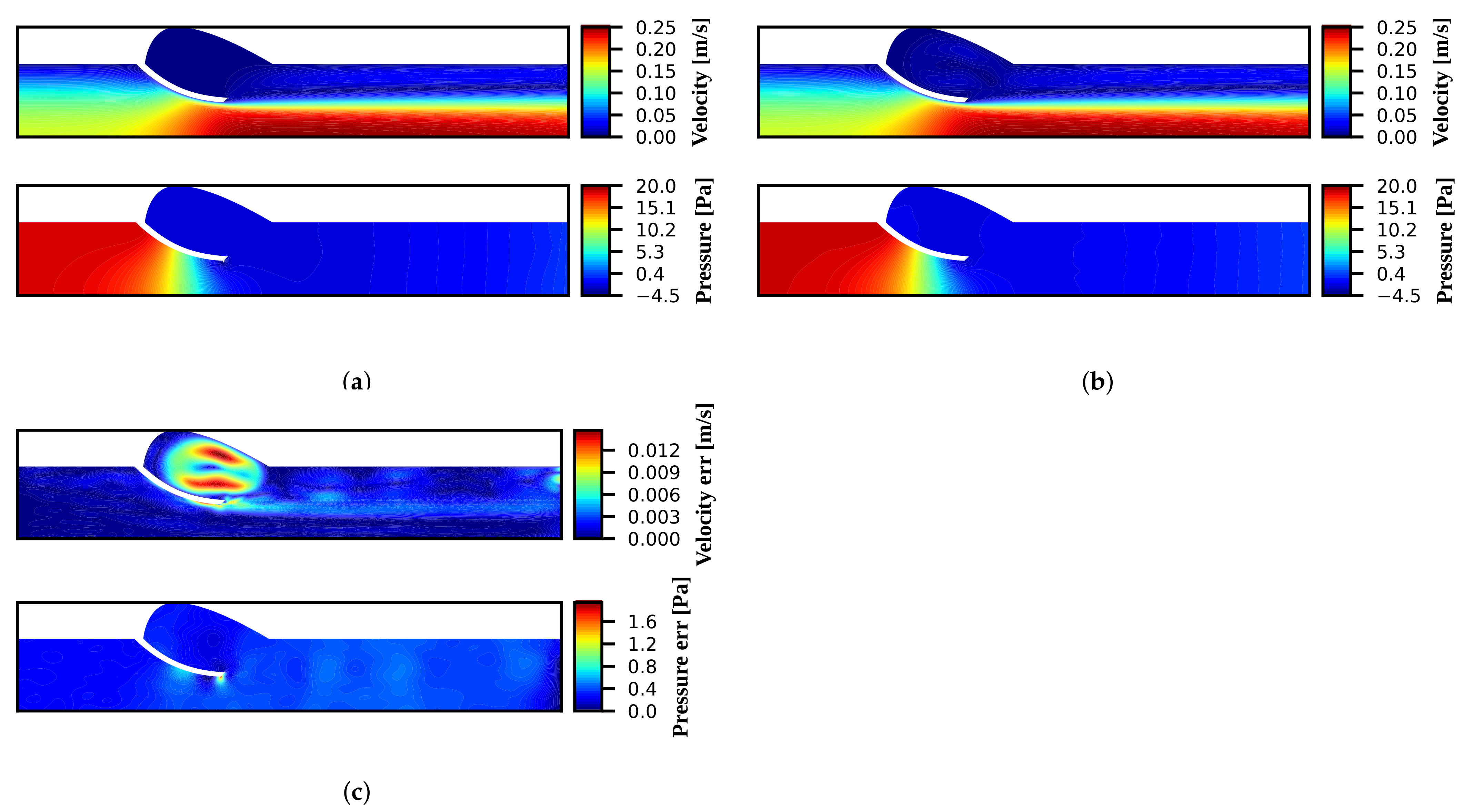
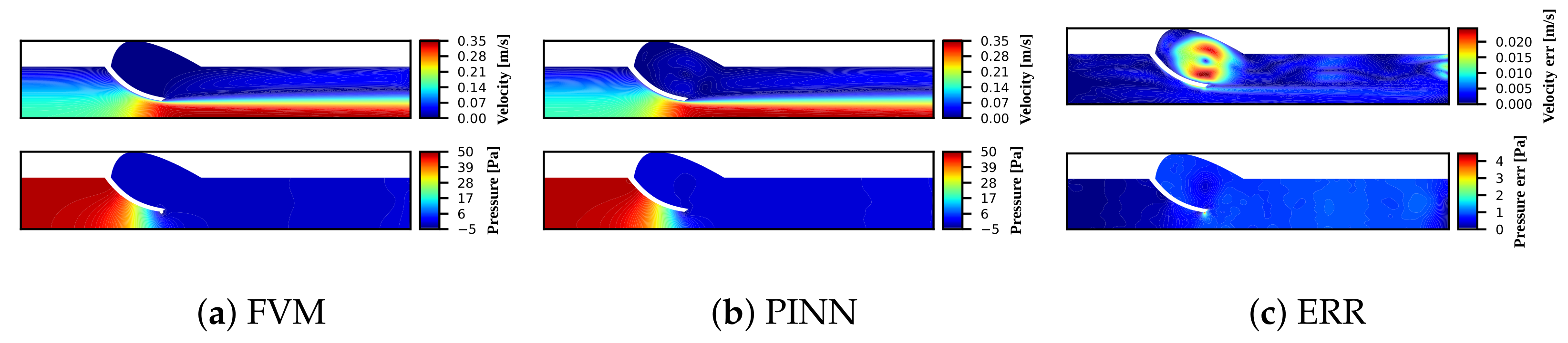
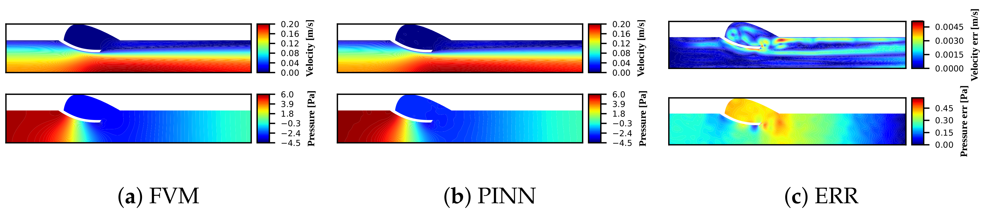
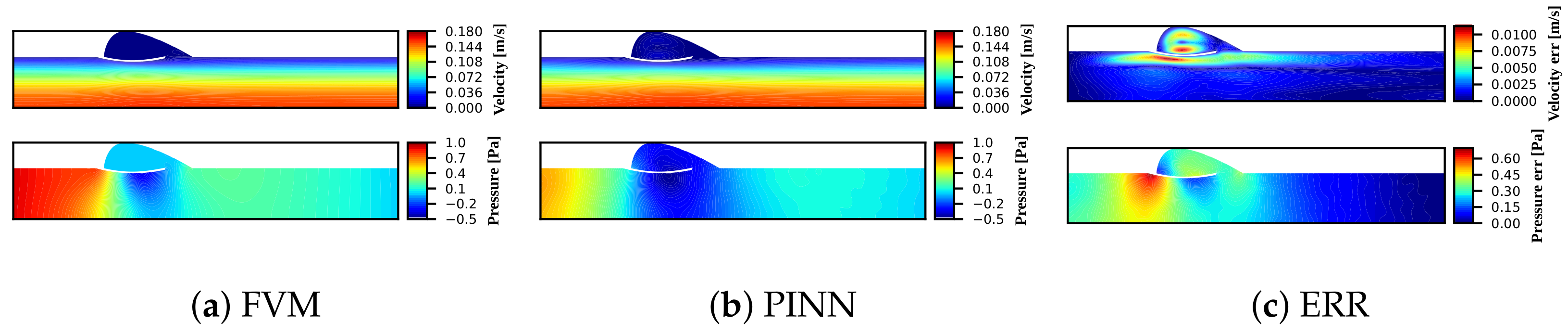
The pressure and velocity fields for a valve angle of 45${}^{\circ }$ are shown in Figure 10 for the PINN and FVM, as well as the absolute difference between the two. The figures for the other valve angles are shown in Appendix A. The evaluation metrics are shown in

Table 3. Simulation Cases: FVM.

Valve Angle	Peak Jet Velocity	Pressure Drop	Simulation Time
[deg]	[m/s]	[Pa]	[s]
35	0.3386	47.47	36.452
45	0.2465	18.17	38.782
55	0.195	5.621	25.357
75	0.154	0.8754	19.637

,

Table 4. Simulation Cases: PINN.

Valve Angle	Peak Jet Velocity	Pressure Drop	Momentum Residual	Simulation Time
[deg]	[m/s]	[Pa]		[s]
35	0.3377	47.45	4.69 × 10${}^{-4}$	5010
45	0.2475	18.4	3.11 × 10${}^{-4}$	4515
55	0.1956	5.843	1.13 × 10${}^{-4}$	5172
75	0.1549	0.5956	1.41 × 10${}^{-4}$	5843

and

Table 5. Simulation Cases: error metrics.

Valve Angle	e1	e2	e3	e4
[deg]	[%]	[%]	[%]	[%]
35	0.3757	0.06139	6.691	9.29
45	−0.3016	−1.295	5.736	10.59
55	−0.2521	−3.952	2.612	10.18
75	−0.6278	31.96	7.227	78.57

.

The results show that the PINN solution was in good agreement with the FVM solution. Both the pressure and the velocity fields were closely matched. It can be seen in Figure 10c that the PINN solution showed a circulation action in the sinus that was not present in the FVM solution. The physicality of this circulation action was difficult to verify without experimental data; however, we intuitively expected some circulating flow in the sinus, due to the shearing action of the jet: if this intuition was correct, then the PINN solution was representative of the actual flow.

Table 3 and Table 5 show that both the PINN and FVM predicted an increase in the peak jet velocity and pressure drop as the flow restriction was increased. Notably, the PINN simulation time was significantly longer than that of the FVM: this was to be expected with the current state of the art in PINN research for this type of problem. Both the PINN and FVM showed slower convergence with increasing flow restriction.

Table 5 shows that the velocity field was in much better agreement between the PINN and FVM than the pressure field. The peak jet velocity errors ($e_1$) were all below $1\%$, whereas three of the pressure drop errors ($e_2$) were above $1\%$. The pressure drop error for a valve angle of 35${}^{\circ }$ was substantially lower than the other errors, for both the laminar and turbulent solutions. We consider this result to be an outlier, especially as the maximum absolute error of the pressure field ($e_4$) was not that much smaller than the $e_4$ errors of the other valve angles. The pressure drop error ($e_2$ ) and maximum absolute error of the pressure field ($e_4$), for a valve angle of 75${}^{\circ }$, were much larger than the other errors: this was because there was very little flow restriction in this case, which resulted in a very small pressure drop. The PINN training process is biased towards resolving features that have a larger impact on the numerical values in the loss function. When there is little flow restriction, the pressure gradient term in the momentum residual function is small, and the PINN training process resolves the pressure field more slowly.

Overall, the velocity field results are in better agreement than the pressure field results: this was somewhat expected, as although the $\psi -p$ formulation used for the PINN ensured perfect mass conservation, there remained a residual in the momentum conservation equation. Momentum conservation ensured the dynamic equilibrium of forces in the system, which the pressure and velocity fields contributed to; however, it seems that the pressure field was more sensitive to errors in the momentum conservation equation than the velocity field.

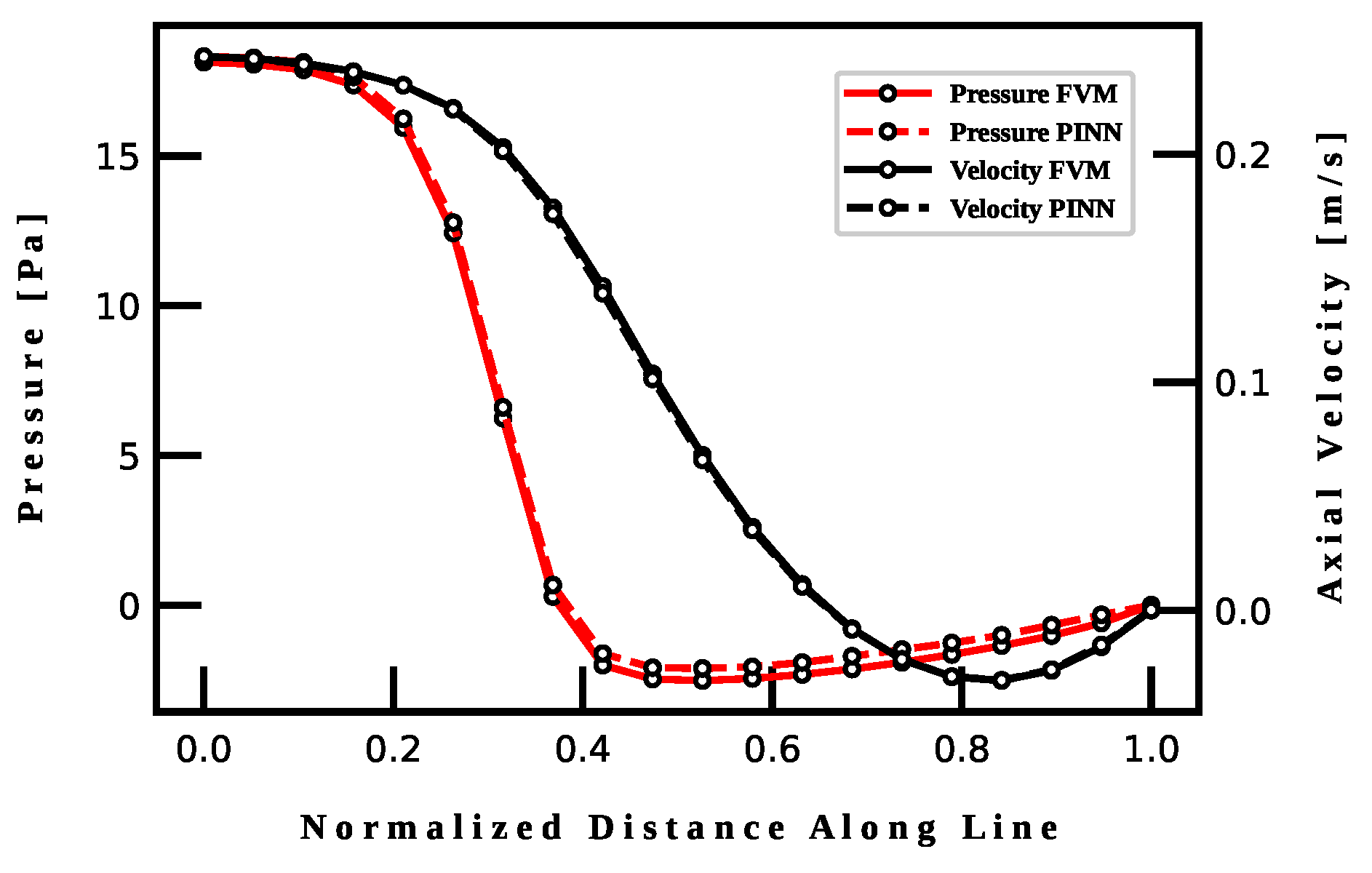
The section plots shown in Figure 11 illustrate good agreement between the predicted pressure and velocity fields by the FVM and PINN methods. The velocity profile predicted by the PINN, shown in a black dashed line, is difficult to distinguish from the profile predicted by the FVM, shown in a solid black line, due to them being so closely matched. Both methods predict an s-shaped velocity profile, with some reversed flow near the wall of the vessel.

The pressure profiles, shown in red, are less closely matched, but still difficult to distinguish. Both methods predict a sharp pressure drop at the valve, followed by a small amount of pressure recovery downstream of the valve, as the steady velocity profile starts to develop and the maximum jet velocity decreases.

5.2. Turbulent Flow

Flow in the turbulent regime was also simulated for a range of valve angles between 75${}^{\circ }$ and 35${}^{\circ }$. A parabolic inlet velocity profile was used, at a volumetric flow rate of 400 mL/s: this flow rate corresponded to the peak systolic flow rate of a healthy adult male [37]. At this volume flow rate, the Reynolds number based on the base diameter was $Re=5438$, which was below the critical Reynolds number for a tube. The flow did, however, transition to turbulence, due to the presence of the valve.

Similarly to the laminar model setup, a four-layer neural network was used, with 20 neurons in each layer, except for the Fourier encoding layer, which had 40 neurons. The network was trained for 10,000 epochs, using the ADAM optimizer with a mini-batch size of 1024 and a learning rate of 1 × 10${}^{-3}$. The momentum conservation loss function and boundary loss functions were evaluated at 8727 and 765 collocation points, respectively.

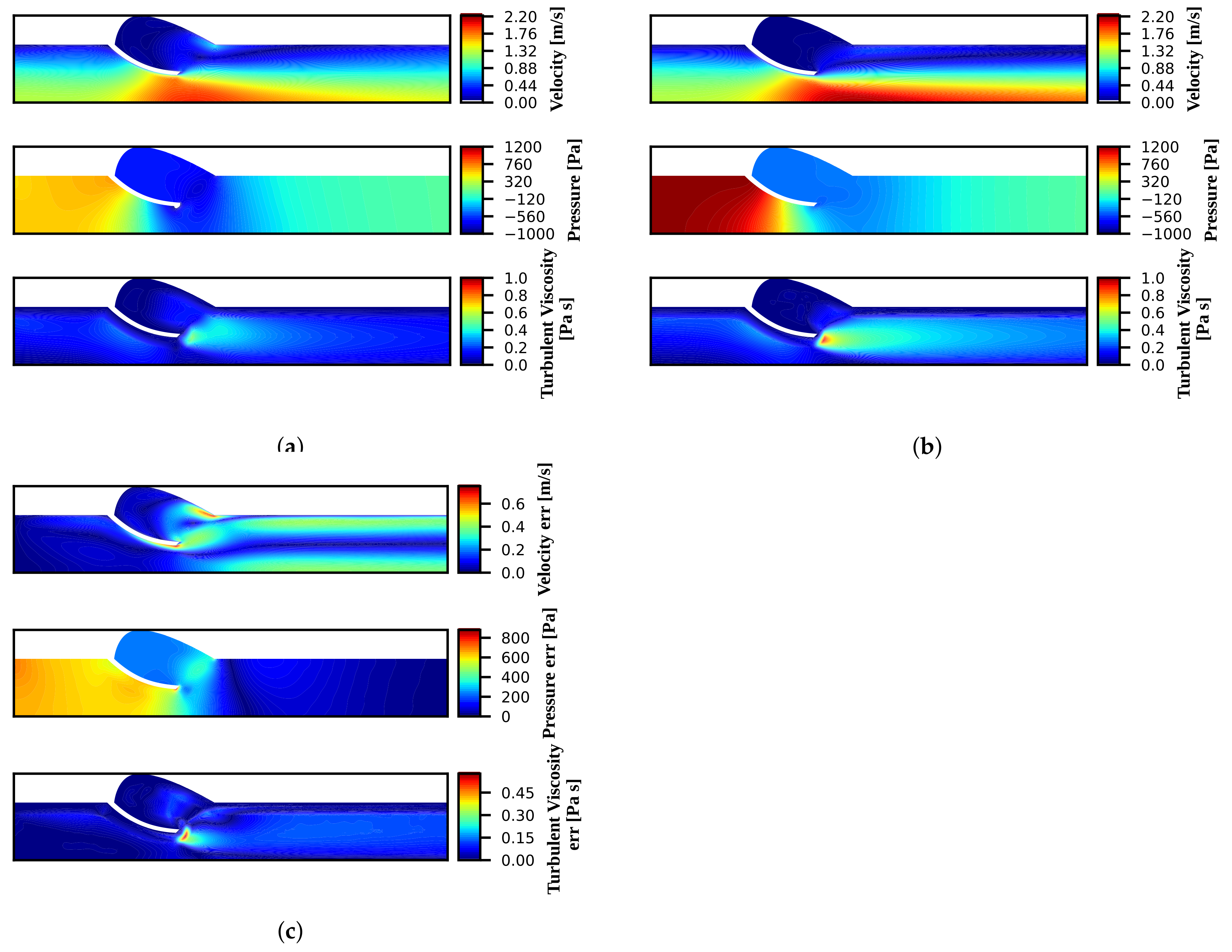
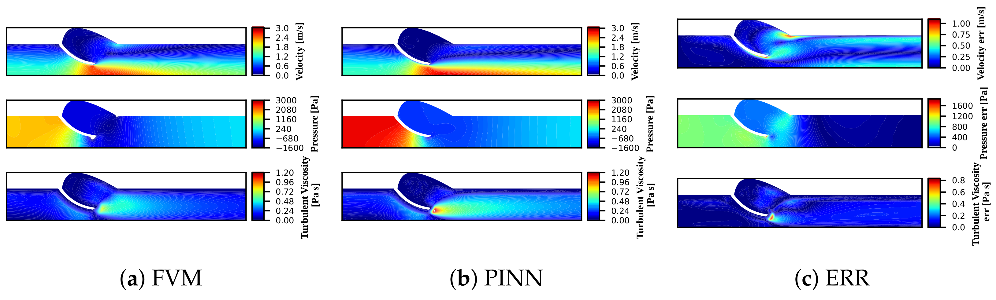
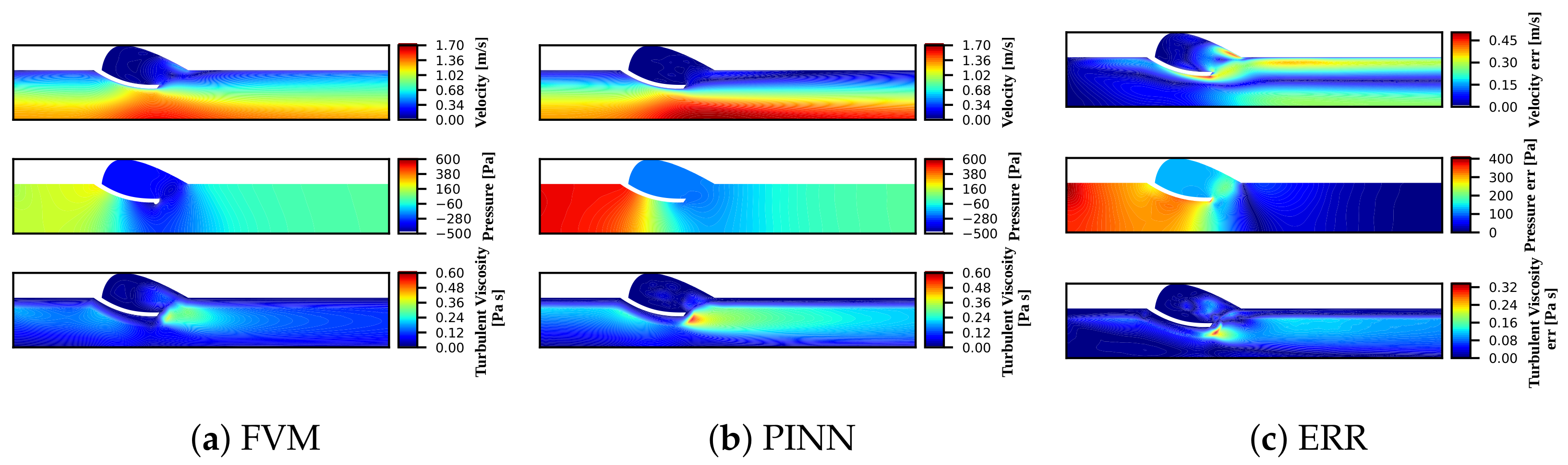
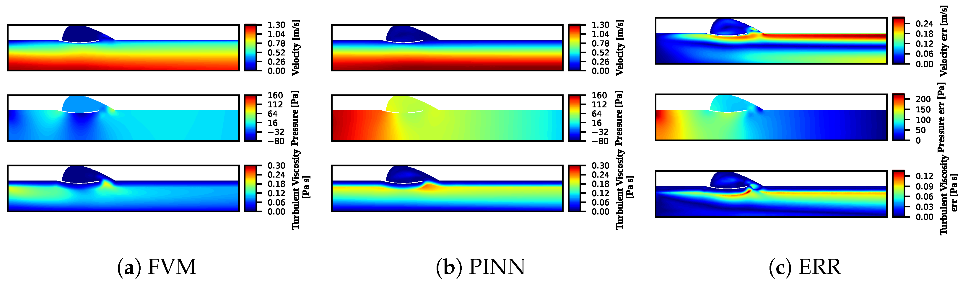
The pressure, velocity and turbulent viscosity fields for a valve angle of 45${}^{\circ }$ are shown in Figure 12 for the PINN and FVM, as well as the absolute difference between the two. Figures for the other valve angles are shown in Appendix A. The results are also tabulated in

Table 6. Simulation Cases: FVM.

Valve Angle	Peak Jet Velocity	Pressure Drop	Simulation Time
[deg]	[m/s]	[Pa]	[s]
35	2.601	1609.6	642
45	1.906	518.2	613
55	1.531	132.1	299.5
75	1.252	−39.07	278

,

Table 7. Simulation Cases: PINN.

Valve Angle	Peak Jet Velocity	Pressure Drop	Momentum Residual	Simulation Time
[deg]	[m/s]	[Pa]		[s]
35	2.744	2557.2	1.74 × 10${}^{-3}$	10,002
45	2.103	1173.6	3.31 × 10${}^{-4}$	12,321
55	1.667	502.1	1.36 × 10${}^{-4}$	10,166
75	1.318	150.0	5.41 × 10${}^{-5}$	9234

and

Table 8. Simulation Cases: error metrics.

Valve Angle	e1	e2	e3	e4
[deg]	[%]	[%]	[%]	[%]
35	−5.529	−58.87	41.82	112.9
45	−10.34	−126.5	39.04	157.6
55	−8.93	−280.2	32.86	241.7
75	−5.312	484.0	21.58	−4168

.

The results show that the addition of a mixing length turbulence model to the PINN enabled the simulation of steady turbulent flows; however, the PINN solution did not match the FVM solution as well as it matched the laminar case: here, the FVM solution predicted more circulation in the sinus area than did the PINN, as shown in Figure 12c. Both methods predicted a region of high turbulent viscosity near the tip of the valve leaflet, but the PINN predicted a higher viscosity than the FVM.

Looking at Table 6 and Table 7, once again both models predicted an increase in the peak jet velocity and pressure drop, as the valve angle decreased. Simulation times were longer for both methods when compared to the laminar case, and the PINN simulations converged more slowly than did the FVM simulations.

The PINN simulation, at a valve angle of 35${}^{\circ }$, terminated with a relatively large momentum residual, compared to the other laminar and turbulent simulations: it seems that the steeper gradients present in this case reduced the training performance of the neural network.

A strange result to note in Table 6 is the negative pressure drop at a valve angle of 75${}^{\circ }$: this was a result of the parabolic inlet velocity profile that was used in place of a fully developed turbulent velocity profile. As a turbulent velocity profile develops, the average velocity remains constant, but the peak velocity decreases: this results in a decrease in the kinetic energy of the mean flow, and an increase in the static pressure, due to Bernoulli’s principle. As the pressure drop due to flow restriction was so small in the 75${}^{\circ }$ case, the pressure gain due to the developing velocity profile was enough to cause a negative pressure drop.

Table 8 shows higher errors across the board for the turbulent case, compared to the laminar case. The peak jet velocity error ($e_1$), pressure drop error ($e_2$), normalized maximum velocity error ($e_3$) and normalized maximum pressure error ($e_4$) had a median increase in error, by a factor of 20, 28, $5.5$ and 18 higher, respectively.

Once again, the PINN was able to infer more accurate velocities than pressures. The median difference in error between the turbulent peak velocity error $e_1$ and the turbulent pressure drop error $e_2$ was 20 times. The median difference in error between the turbulent normalized maximum velocity error $e_3$ and the turbulent normalized maximum pressure error $e_4$ was $3.7$ times.

Median values are quoted instead of mean values because the results were skewed by the large error values for the 75${}^{\circ }$ case. The 75${}^{\circ }$ turbulent case had a larger error for the same reason as the laminar case: the small amount of flow restriction made the pressure term in the momentum equation small, which caused the PINN to resolve the pressure field much more slowly than the velocity field.

Figure 13 provides another perspective on the differences between the turbulent FVM and PINN solutions, along the section lines as defined in Figure 9 for a valve angle of 45${}^{\circ }$.

Based on the velocity profiles, shown in black, it can be seen that the PINN predicted less diffusion in the jet than the FVM. The PINN predicted some backflow near the wall, whereas the FVM did not.

The pressure curves, plotted in red, show a sharp drop in pressure at the valve, with a much faster recovery downstream than the laminar case (Figure 11): this is seen in the PINN and FVM solutions, but the FVM solution shows a faster pressure recovery than the PINN.

6. Conclusions

In this paper, we have demonstrated the application of Physics-Informed Neural Networks as a new deep-learning-based method for solving the incompressible Reynolds-averaged Navier–Stokes equations in a biomedical context. Transvalvular blood flow was simulated in the laminar and turbulent regimes, with a varying degree of simulated valve stenosis. Various methods of improving the training performance and prediction accuracy of PINNs, from the literature, were implemented, including the Gradient-Enhanced PINN [19], the Fourier encoding layer [20] and the re-introduction of spatial information using skip connections [7]. A mixing length turbulence closure model was implemented for the turbulent case. The mixing length was calculated by solving a Poisson-type equation with a secondary PINN to calculate the normal wall distance.

The PINN method was found to be able to accurately simulate the laminar flow case, but the method seemed to be sensitive to the specific problem geometry: at valve angles of 35${}^{\circ }$ to 55${}^{\circ }$, the error values ranged between 0.2521% and 6.691% for the velocity field, and 0.06139% and 10.59% for the pressure field; at a valve angle of 75${}^{\circ }$, the error values were as large as 7.227% and 78.57% for the velocity field and pressure field, respectively.

The PINN method matched the FVM solution in the turbulent regime, qualitatively, which is a promising result; however, quantitative accuracy will need to improve substantially for this methodology to be a useful scientific tool in this regime. At higher degrees of stenosis, with valve angles between 35${}^{\circ }$ and 55${}^{\circ }$, the error values ranged between 5.529% and 41.82% for the velocity field, and between 58.87% and 280.2% for the pressure field. At a valve angle of 75${}^{\circ }$, the velocity and pressure errors were as large as 21.58% and 4168%, respectively.

The general trend seems to be that the PINN method was able to infer more accurate velocity fields than pressure fields: this is likely, as the $\psi -p$ formulation of the Navier–Stokes equations was used, which enforces continuity exactly, but leaves a finite residual in the momentum equation. Thus, we observed that the pressure field was more sensitive to errors in the momentum equation than was the velocity field.

Simulation times were significantly longer with the PINN method than with the FVM, with the PINN taking up to two orders of magnitude longer to converge than did the FVM code. This currently makes PINNs an unattractive option in a scenario like the one presented in this paper, where a well-posed, non-parametric problem must be solved. Much research is being done to understand and improve the training dynamics of PINNs [20,38,39], which will hopefully lead to a more efficient training process. The authors also note that in this study, accuracy was prioritized over computational efficiency, and that the custom code used for the PINN was not pre-compiled or optimized.

The PINN method becomes much more attractive when the problem is ill-posed: for example, the problem of simulating transvalvular flow, where the inlet boundary condition is unknown but some sparse velocity measurements can be taken by using 4D flow MRI. Solving such a problem with the FVM requires a post-optimization procedure that is currently impossible, due to its computational expense. With the PINN method, however, the solution time is approximately the same as, or faster than, the well-posed, data-less case.

Once a PINN is trained, inference can be performed in real time with little computational expense: this makes PINNs a good candidate for use in real-time monitoring and control systems, as a surrogate model. Another advantage of using PINNs as surrogate models is that known physics is enforced, allowing for more reliable extrapolation, if that is required. PINNs also offer favorable scaling of the computational expense of constructing surrogate models for parameterized problems, because the solution is computed across the parameter range in parallel: this means that considerable speedup can be achieved for highly parameterized problems.

Future work in PINNs research should include further improvement of the numerics of PINNs. As noted above, PINNs suffer from numerical stiffness of the training dynamics, and it has been shown that a substantial reduction in the training time, and improvement in the prediction accuracy, can be achieved by improving the numerics of the PINN methodology. Such improvements can be achieved with alternative network architectures, such as convolutional neural networks (CNNs) [40] or graph neural networks (GNNs): these architectures are expected to perform better, because they introduce a sense of locality to the network. The information from collocation points that are close together interacts differently in these networks than does the information from collocation points that are far apart: this mirrors how regions of fluid that are close together interact differently than regions of fluid that are far apart. Future work should also include further investigation of methods for performing automatic weighting of the loss function terms. Some work has been done in this area [39,41], but more work is needed, to find a method that works well for all problems. Finally, the authors believe that some fundamental research is needed to understand why PINNs perform so poorly, with the formulation used in this paper, in the turbulent regime.