Spatio-Temporal Gradient Enhanced Surrogate Modeling Strategies

Abstract

This research compares the performance of space-time surrogate models (STSMs) and network surrogate models (NSMs). Specifically, when the system response varies over time (or pseudo-time), the surrogates must predict the system response. A surrogate model is used to approximate the response of computationally expensive spatial and temporal fields resulting from some computational mechanics simulations. Within a design context, a surrogate takes a vector of design variables that describe a current design and returns an approximation of the design’s response through a pseudo-time variable. To compare various radial basis function (RBF) surrogate modeling approaches, the prediction of a load displacement path of a snap-through structure is used as an example numerical problem. This work specifically considers the scenario where analytical sensitivities are available directly from the computational mechanics’ solver and therefore gradient enhanced surrogates are constructed. In addition, the gradients are used to perform a domain transformation preprocessing step to construct surrogate models in a more isotropic domain, which is conducive to RBFs. This work demonstrates that although the gradient-based domain transformation scheme offers a significant improvement to the performance of the space-time surrogate models (STSMs), the network surrogate model (NSM) is far more robust. This research offers explanations for the improved performance of NSMs over STSMs and recommends future research to improve the performance of STSMs.

1. Introduction

This paper investigates the use and suitability of radial basis function (RBF) surrogate models to predict a system’s response through some pseudo-time variable. This type of problem is often present in computationally expensive computation fluid dynamics (CFD) simulations, crash-worthiness simulations, or pressure control simulations, where a designer wishes to predict the change in a design’s behavior without recomputing a computationally expensive simulation. Therefore, the surrogate model is intended to replace the computationally expensive simulation by accepting a vector of variables that describe a design and offer a computationally inexpensive approximation of the design’s response through a pseudo-time variable. In this problem, the surrogate model needs to return a continuous approximation as a function of the pseudo-time variable, and not simply a single scalar value as is often the case with surrogate models. Hence, the surrogate needs to return a response vector, which is often referred to as a vector-valued surrogate model [1].

In this work, the scenario where the analytical gradients are available is considered. Many papers [2,3,4,5] detail procedures to calculate the design sensitivities for functions that are computed using the finite element method (FEM) or finite volume method (FVM) for structural mechanics and computational fluid dynamics (CFD). Some finite element packages even have adjoint sensitivities implemented, for example, Calculix [6]. This gradient information can be calculated with respect to many different design variables for a wide range of problems [2,4,7,8,9].

As per usual practice, these analytical sensitivities are used directly in the RBF surface approximation, i.e., to construct gradient enhanced RBF models (GE-RBF) [10,11]. In addition, these sensitivities are used to perform a domain transformation preprocessing step that aims to find a transformation that results in a near isotropic surface to be approximated. This domain transformation step was previously developed by the authors to accommodate the application of RBF kernels that are isotropic on the approximation of non-isotropic surfaces often resulting in engineering problems [12,13,14,15]. This is discussed in more detail later in the paper in Section 2.

There are two main options for constructing a surrogate model that can predict behavior through a pseudo-time variable. Firstly, the design variables and the pseudo-time variable can be uncoupled, and a network of smaller surrogate models can be constructed and trained at m predetermined locations in the pseudo-time variable. In order to sample the approximated behavior, each RBF model is then sampled separately, and some interpolation scheme is used to find the result at locations other than the m pseudo-time points. In this work, simple linear interpolation is implemented. This surrogate model approach is referred to as the network surrogate model (NSM) [16].

The second option is to couple the design and pseudo-time variables and construct one surrogate model over the shape and pseudo-time variables. Such a surrogate model is often referred to as a space-time or spatio-temporal surrogate model (STSM) [17,18,19]. RBF is a popular choice for the construction of STSMs, and is used in this study. Hence, from here onwards, STSM will imply an RBF-constructed STSM. This option has the benefit of being easier to implement, as only one model needs to be trained, whereas, for the NSM, m models need to be trained. However, as will be demonstrated in this paper, if the limitations of the RBF model are not properly understood and addressed, the STSM may offer inferior predictive performance when compared to the NSM.

To assess the surrogate models in this work, the models are used to predict the load-displacement paths of snap-through structures as a function of various shape parameters. As the load paths of the structures are highly non-linear, the finite element method (FEM) simulation needs to be completed with the arc length control (ALC) method [20]. The ALC method introduces a pseudo-time variable, commonly referred to as the arc length, to allow the calculation of force–displacement curves.

The analytical sensitivity procedure used in this research to compute sensitivities has been completed previously by the authors [21]. Specifically, the assumed stress element in conjunction with the ALC method is used to simulate the behavior of snap-through structures.

The layout of this paper is then as follows. Firstly, a brief mathematical description of RBF surrogate models is offered in Section 2, where the use of gradient information, both directly in the model itself and as a preprocessing step, is also detailed. This section also describes the NSM and STSMs in more detail. In Section 3, a more detailed description of snap-through structures’ behavior as well as the required ALC solution strategy is described. From the description in Section 3, the numerical problem of predicting the load path of these structures is presented in Section 4. The numerical results are detailed in Section 5, where the models are used to predict the load–displacement curves of the selected snap-through mechanism. This is followed by observations and conclusions in Section 6.

2. RBF Surrogate Models

Surrogate model construction can broadly be separated into the following steps:

• Domain sampling;
• Preprocessing;
• Model selection or construction;
• Model prediction.

Each of these steps is a research topic by itself, where various methods or algorithms have been developed to produce optimal results. In this research, each of the steps is completed with the most standard or common method, as the goal of the paper is to isolate the effects of the preprocessing step.

Radial basis function surrogate models refer to a group of models that use a linear summation of basis functions that usually depend on some non-linear distance measure between two points. Popular options as basis functions include the following:

• Inverse quadratic: $\varphi (\mathit{x},\mathit{c},ϵ)=\frac{1}{1+ϵ\left|\right|\mathit{x}-{\mathit{c}\left|\right|}^2}$,
• Multi-quadratic: $\varphi (\mathit{x},\mathit{c},ϵ)=\sqrt{\left|\right|\mathit{x}-{\mathit{c}\left|\right|}^2+{ϵ}^2}$,
• Gaussian: $\varphi (\mathit{x},\mathit{c},ϵ)=e^{-ϵ\left|\right|\mathit{x}-{\mathit{c}\left|\right|}^2}$,

where the variables $\mathit{x}$, $ϵ$, $\mathit{c}$ are the sampled point in design space, the center of the basis function, and the shape parameter, respectively. A widely used basis function is the Gaussian function [11,22,23], which is the basis function used in this research. The RBF surrogate is expressed as a linear combination of K basis functions

$$f_{\mathrm{RBF}}=\sum _{i=1}^K{w}_i\varphi (\mathit{x},{\mathit{c}}_i,ϵ).$$

(1)

This can be expressed as a system of equations

$$\mathit{f}=\mathit{M}(\mathit{x},\mathit{c},ϵ)\mathit{w},$$

(2)

where the goal of fitting the surrogate model refers to finding the optimal values of the weight vector $\mathit{w}$. The matrix $\mathit{M}$ is expressed as

$$\mathit{M}=\left[\begin{array}{cccc}\varphi ({\mathit{x}}_1,{\mathit{c}}_1,ϵ)& \varphi ({\mathit{x}}_1,{\mathit{c}}_2,ϵ)& \cdots & \varphi ({\mathit{x}}_1,{\mathit{c}}_K,ϵ)\\ \varphi ({\mathit{x}}_2,{\mathit{c}}_1,ϵ)& \varphi ({\mathit{x}}_2,{\mathit{c}}_2,ϵ)& \cdots & \varphi ({\mathit{x}}_2,{\mathit{c}}_K,ϵ)\\ ⋮& ⋮& ⋮& ⋮\\ \varphi ({\mathit{x}}_p,{\mathit{c}}_1,ϵ)& \varphi ({\mathit{x}}_p,{\mathit{c}}_2,ϵ)& \cdots & \varphi ({\mathit{x}}_p,{\mathit{c}}_K,ϵ)\end{array}\right].$$

(3)

The size of matrix $\mathit{M}$ is, therefore, $p\times K$, where p is the number of samples in the design space, and K is the number of centers or basis functions used in the model. The methods for determining the locations of the samples in the construction space are discussed in Section 2.3.

The remaining parameters of the surrogate include the number and locations of the centers $\mathit{c}$ and the value of the shape parameter $ϵ$. A popular choice for the centers is to select $p=K$, meaning that the number of centers is equal to the number of sampled points and to position the centers at the location of the sampled points [11]. For this choice, the matrix $\mathit{M}$ becomes square, and the weight vector can be solved directly from Equation (2). This is the option that is implemented in this research.

The shape parameter can either be determined with some heuristic [24], or with a k-fold cross-validation or leave-one-out cross-validation (LOOCV) approach [11,23]. In this research, various shape parameters between ${10}^{-2}$ and ${10}^1$ are evaluated using k-fold cross validation as a metric, and the shape parameter associated with the lowest error is selected.

2.1. Direct Gradient Enhancement

The so-called gradient enhanced RBF (GE-RBF) surrogate model is implemented in this research [10]. The usual function-value-only RBF model can be expanded to include gradient information in its construction [11]. This can be done by first taking the gradient of the chosen basis function

$${\frac{d\varphi (\mathit{x},\mathit{c},ϵ)}{d\mathit{x}}}^T=-2ϵ\varphi (\mathit{x},\mathit{c},ϵ)(\mathit{x}-\mathit{c}),$$

(4)

where Equation (4) returns a column vector of the gradients of the RBF basis functions [11].

A new system of equations can then be created from the gradient information at each sampled point for the p samples of the RBF surrogate model [11]:

$$\left[\begin{array}{c}\frac{d{f}_1}{d\mathit{x}}\\ \frac{d{f}_2}{d\mathit{x}}\\ ⋮\\ \frac{d{f}_p}{d\mathit{x}}\end{array}\right]=\left[\begin{array}{cccc}\frac{d\varphi ({\mathit{x}}_1,{\mathit{c}}_1,ϵ)}{d\mathit{x}}& \frac{d\varphi ({\mathit{x}}_1,{\mathit{c}}_2,ϵ)}{d\mathit{x}}& \cdots & \frac{d\varphi ({\mathit{x}}_1,{\mathit{c}}_K,ϵ)}{d\mathit{x}}\\ \frac{d\varphi ({\mathit{x}}_2,{\mathit{c}}_1,ϵ)}{d\mathit{x}}& \frac{d\varphi ({\mathit{x}}_2,{\mathit{c}}_2,ϵ)}{d\mathit{x}}& \cdots & \frac{d\varphi ({\mathit{x}}_2,{\mathit{c}}_K,ϵ)}{d\mathit{x}}\\ ⋮& ⋮& ⋮\\ \frac{d\varphi ({\mathit{x}}_p,{\mathit{c}}_1,ϵ)}{d\mathit{x}}& \frac{d\varphi ({\mathit{x}}_p,{\mathit{c}}_2,ϵ)}{d\mathit{x}}& \cdots & \frac{d\varphi ({\mathit{x}}_p,{\mathit{c}}_K,ϵ)}{d\mathit{x}}\end{array}\right]\left[\begin{array}{c}{w}_1\\ w_2\\ ⋮\\ w_K\end{array}\right].$$

(5)

This system can then be written as

$${\mathit{f}}_{fo}={\mathit{M}}_{fo}{\mathit{w}}_{fo}.$$

(6)

The subscript $fo$ denotes that the first-order information is used in the system. The gradient information can then be combined with the original function-value-only system, Equation (2), to create a new system of equations:

$$\left[\begin{array}{c}\mathit{f}\\ {\mathit{f}}_{fo}\end{array}\right]=\left[\begin{array}{c}\mathit{M}\\ {\mathit{M}}_{fo}\end{array}\right]{\mathit{w}}_{GE}.$$

(7)

The weight vector now contains the subscript $GE$ to show that the weights solved from this system are for the gradient-enhanced versions of the surrogate models. Equation (7) can then be expressed as

$${\mathit{f}}_{GE}={\mathit{M}}_{GE}{\mathit{w}}_{GE}.$$

(8)

An important characteristic to note of the GE models is the size of the system that needs to be solved. In the function-value-based models, p scalar samples are taken of the underlying function, creating a system of size $p\times K$, while in the GE models, p scalars and p gradient vectors of size $n\times 1$ are sampled, as each sampled point contains gradient information, creating a $(p+p\times n)\times K$ system [11]. As the weight vector, ${\mathit{W}}_{GE}$, is the same size, specifically $K\times 1$, in both the function and GE models, and the system is, therefore, over-determined [11]. The difference between the function and GE models is therefore that the GE models regress through both the zero-order and gradient information [11], often conducted using some least squares formulation:

$${\mathit{M}}_{GE}^T{\mathit{f}}_{GE}={\mathit{M}}_{GE}^T{\mathit{M}}_{GE}{\mathit{w}}_{GE}.$$

(9)

2.2. Gradient Based Domain Transformation

Typically, the domain over which the RBF surrogate model is constructed is the result of a simple min-max scaling of the design domain as a preprocessing step [23]. This is done by

$$x_s=\frac{x-x_{min}}{x_{max}-x_{min}},$$

(10)

for each design variable. Here, $x_s$ is the scaled construction domain of the surrogate model, $x_{min}$ is the minimum value of the design variable, and $x_{max}$ is the maximum value of the design variable.

On the other hand, previous work by the authors demonstrated that making use of the gradient information to approximate the underlying curvature of the function can greatly improve the predictive performance of the RBF model [25]. This is due to the fact that RBF models often make the implicit assumption that the underlying function is isotropic which is often not a suitable assumption in many practical engineering problems. Work to address the isotropic problem includes using neural networks, Gaussian mixture models, or sub-space methods [26,27]. In this work, the authors select to handle the isotropic problem using their developed preprocessing procedure.

The proposed method developed by the authors makes use of the gradient information to approximate the underlying curvature and recast the problem into a domain, where the isotropic assumption is more appropriate by completing a full transformation, i.e., a rotation and scaling, of the domain as a preprocessing step.

The method can be broken into the following steps:

• For each center point $\mathit{c}$:

  (a)

  Find the $n+1$ closest points to the center in the sampled points;

  (b)

  Complete a Symmetric Rank 1 approximation of the local curvature or Hessian [11];

  (c)

  Find the eigenvalues and eigenvectors of the local Hessian;

  (d)

  Recalculate the local Hessian with the absolute value of the eigenvalues.

• Find the average local Hessian from the collection of absolute Hessians.
• Calculate the eigenvalues and eigenvectors of the average Hessian.
• Rotate the domain using the eigenvectors and scale with the eigenvalues of the average Hessian.

This method was shown to recover the ideal reference frame and scaling, for a benchmark problem that is decomposable in a rotated frame [25].

2.3. Sampling Methods

Typically the locations of the samples for the construction of the RBF surrogate model are determined with some Latin hyper-cube sampling (LHS) method [11,22]. The standard LHS method is shown in Figure 1 for an increasing number of samples in two dimensions.

The standard LHS method can be improved upon by adding additional constraints to the method such as maximizing the minimum distances between nearest neighbors or incorporating Halton sequences [23]. In this research, the sampling strategy is limited to the simplest version of LHS, as the goal of the paper is to isolate the effects that appropriate domain transformation have on NSM and STSM.

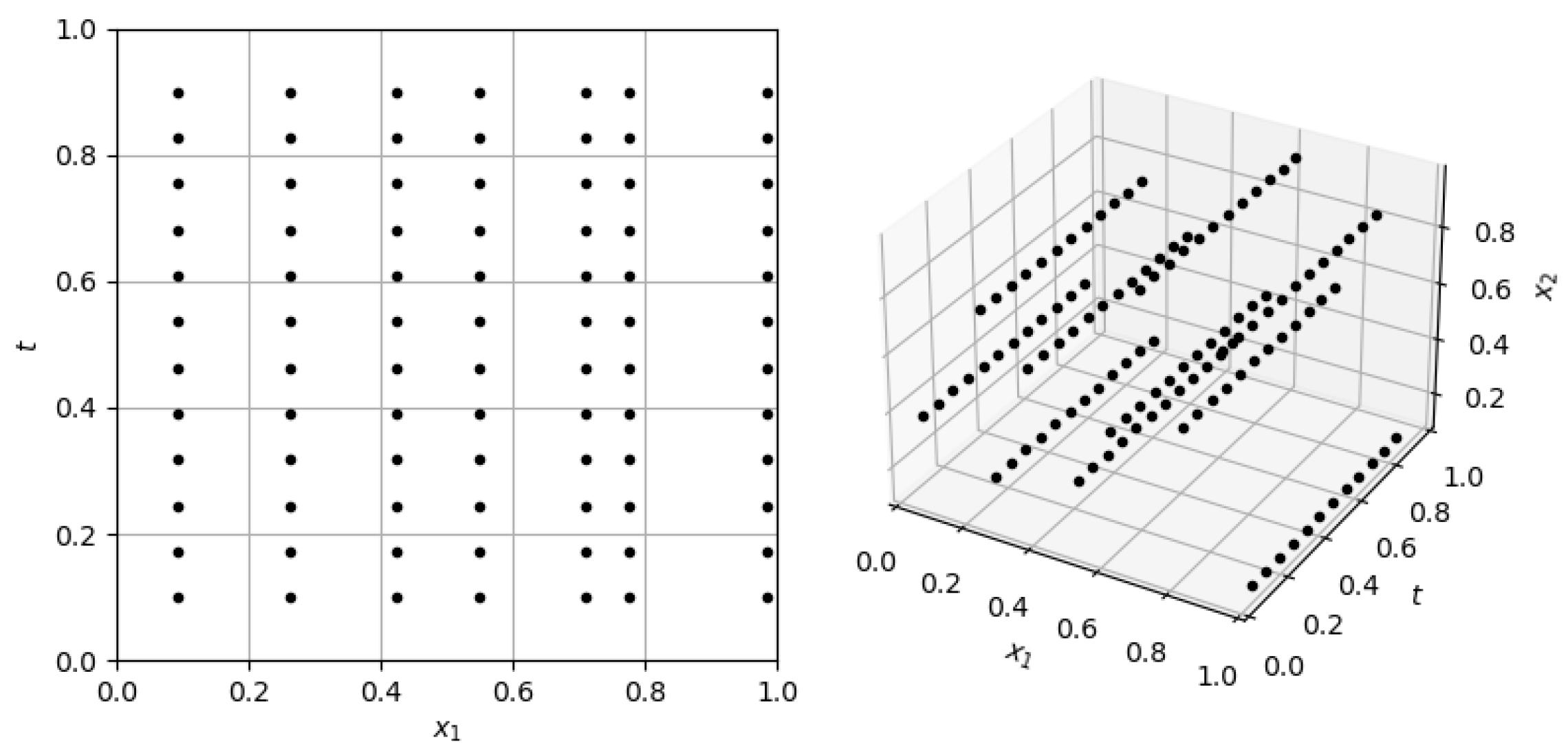
In addition to the LHS method, in this work, the sampling of the pseudo-time variable is completed during some numerical simulation using an iterative solver. This means that the designer has little or no control over the locations, or the number, in the case of an adaptive solver, of samples in this domain. This creates a non-uniform sampling scheme as demonstrated in Figure 2, where design problems with a pseudo-time variable are sampled.

2.4. Network (NSMs) and Space-Time Surrogate Models (STSMs)

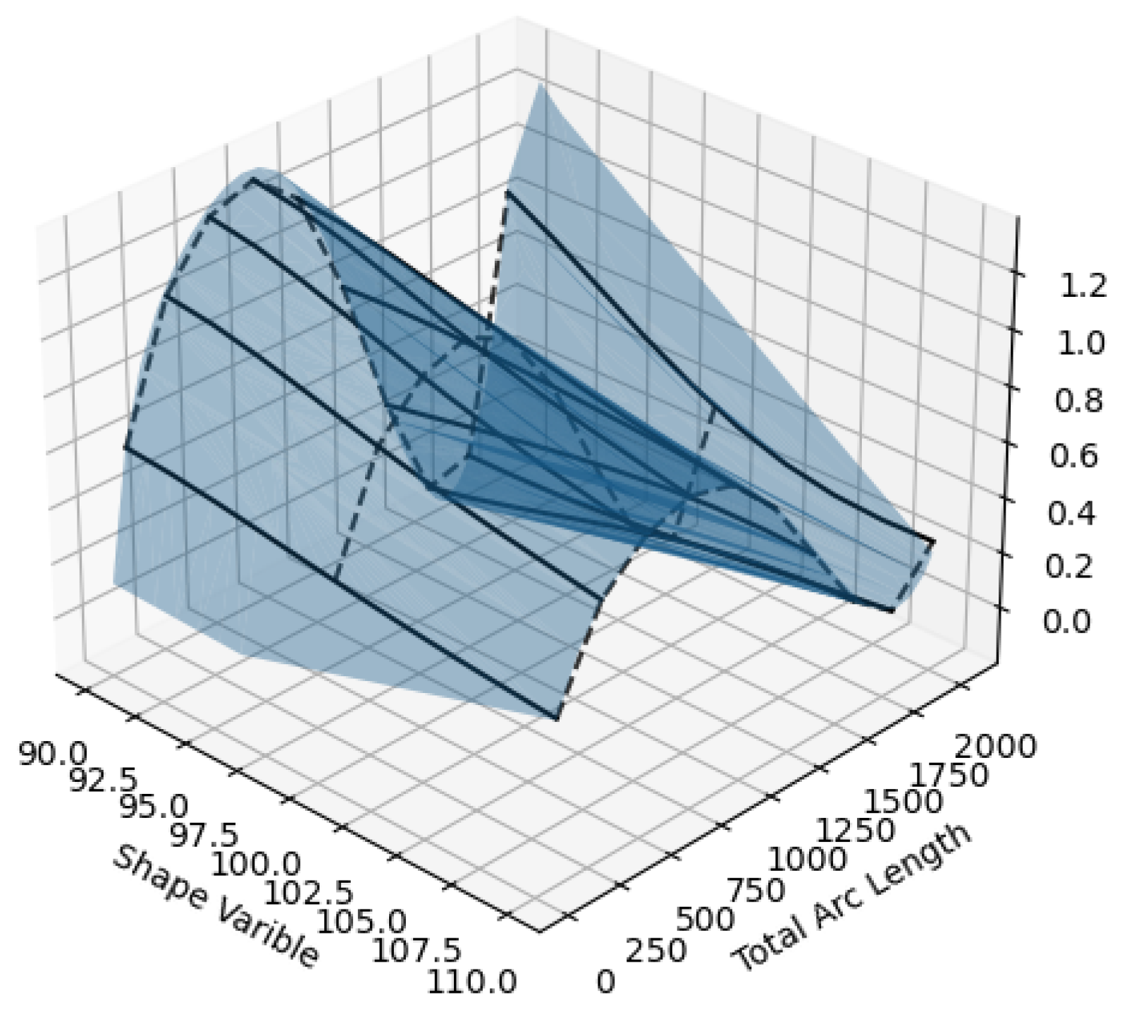
The surrogate models in this work need to return a continuous approximation of a result through a pseudo-time variable. The first method is to uncouple the design and pseudo-time variables and construct multiple smaller RBF models at predetermined locations in the pseudo-time variable. This is represented visually in Figure 3.

The designer needs to determine the number of smaller RBF models as well as their locations in the pseudo-time domain. These decisions are problem specific. As more locations in the pseudo-time variable are selected to have an RBF model, the more flexible the final approximations of the behavior will be but the more computationally expensive the training of the surrogate model becomes.

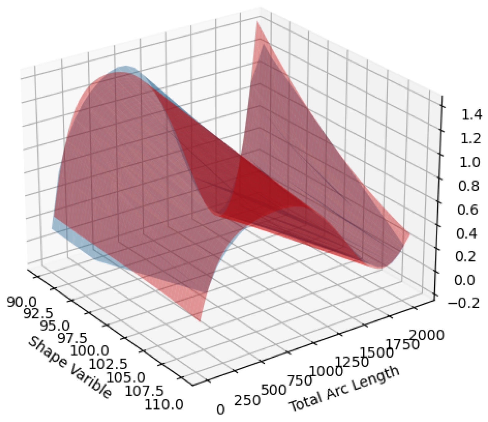
On the other hand, STSM couples the design and pseudo-time variables into one large surrogate model. This method is represented visually in Figure 4 on the same underlying function as for the NSM in Figure 3.

Another key difference that is highlighted in this research between the two models is how they make use of gradient information during their construction. The NSM is only constructed in the design variable domain and therefore cannot make use of the gradient information with respect to the pseudo-time variable. Once all the network RBFs are evaluated at a specific point in pseudo-time, it would be possible to construct some interpolation scheme that uses the gradient information with respect to the pseudo-time variable. In this paper, the linear interpolation in the pseudo-time variable does not use the available gradient information in this direction. On the other hand, the STSM is constructed in both domains, and can therefore make use of all the gradient information present in the problem.

3. Simulating Snap-Through Behavior

Snap-through structures are compliant mechanisms that exhibit highly non-linear load-deflection paths. This means that typical linear finite element solutions strategies are not equipped to fully simulate the structures’ behavior. Instead, a combination of a non-linear solver with the ALC method needs to be implemented in order to accurately predict the structures’ load-displacement path. In typical non-linear FEM analysis, the governing residual equation is expressed as

$$\mathbf{R}=\mathbf{K}\left(\mathbf{u}\right)\mathbf{u}-\lambda \mathbf{F},$$

(11)

where $\mathbf{K}$, $\mathbf{u}$, $\lambda ,$ and $\mathbf{F}$ denote the stiffness matrix, the nodal displacement vector, the load parameter, and the load vector, respectively. In the load control scheme, the goal of some iterative non-linear solver is to find the nodal displacement vector at some load parameter that reduces the governing residual, Equation (11), to $\mathbf{0}$ within some desired tolerance.

This iterative solver typically takes the form of Newton’s method, where the gradient of Equation (11) with respect to the nodal displacement vector is computed. A problem with this solution strategy arises when the load path exhibits a limit point, which is present in snap-through problems, as Newton’s method cannot fully trace the curve past this point.

The ALC algorithm proposes a solution to this problem by adding an additional constraint equation:

$$L^2=▴{\mathbf{u}}^{\mathrm{T}}▴\mathbf{u}+{\psi }^2▴{\lambda }^2{\mathbf{F}}^{\mathrm{T}}\mathbf{F}.$$

(12)

Here, L denotes the prescribed arc length, $▴\mathbf{u}$ is the total displacement vector update for the current load step, $▴\lambda$ is the total load parameter increment for the current load step, and $\psi$ is some non-dimensional scale factor. For a more in-depth description of the ALC algorithm, the reader is referred to literature [20].

The important characteristic of the ALC algorithm that influences this research is that the load and displacement results are now functions of the introduced arc length variable as can be seen in Equation (12). This means that in this research the arc length domain can be treated as a pseudo-time variable when the surrogate models are constructed.

Design Sensitivities

The FEM simulations in this research are completed using the assumed stress element [28] in combination with the ALC method. The assumed stress element is implemented as often snap-through behavior occurs in bending-dominated problems and the assumed stress element returns accurate results in bending problems. Therefore, as the analytical sensitivities are required for this research, the authors implement a procedure developed in previous research, where the same solution strategy was selected [21]. This sensitivity procedure returns the sensitivity information with respect to both the shape variables as well as the arc length variable.

4. Numerical Example

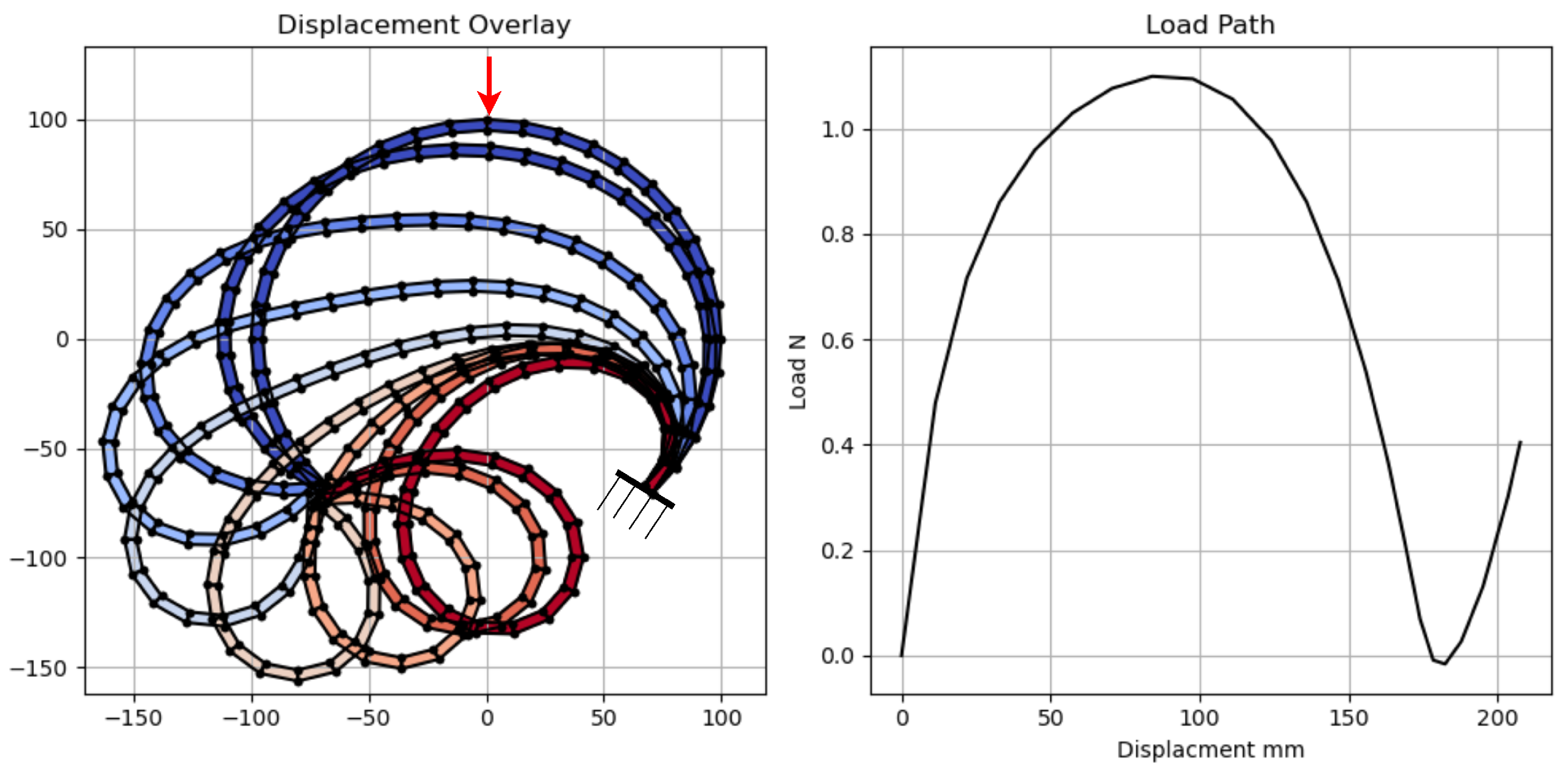
The example problem for this research is to predict the non-linear load path of the so-called deep semi-circular arch [29]. The load-displacement path as well as the deformation overlay is depicted in Figure 5.

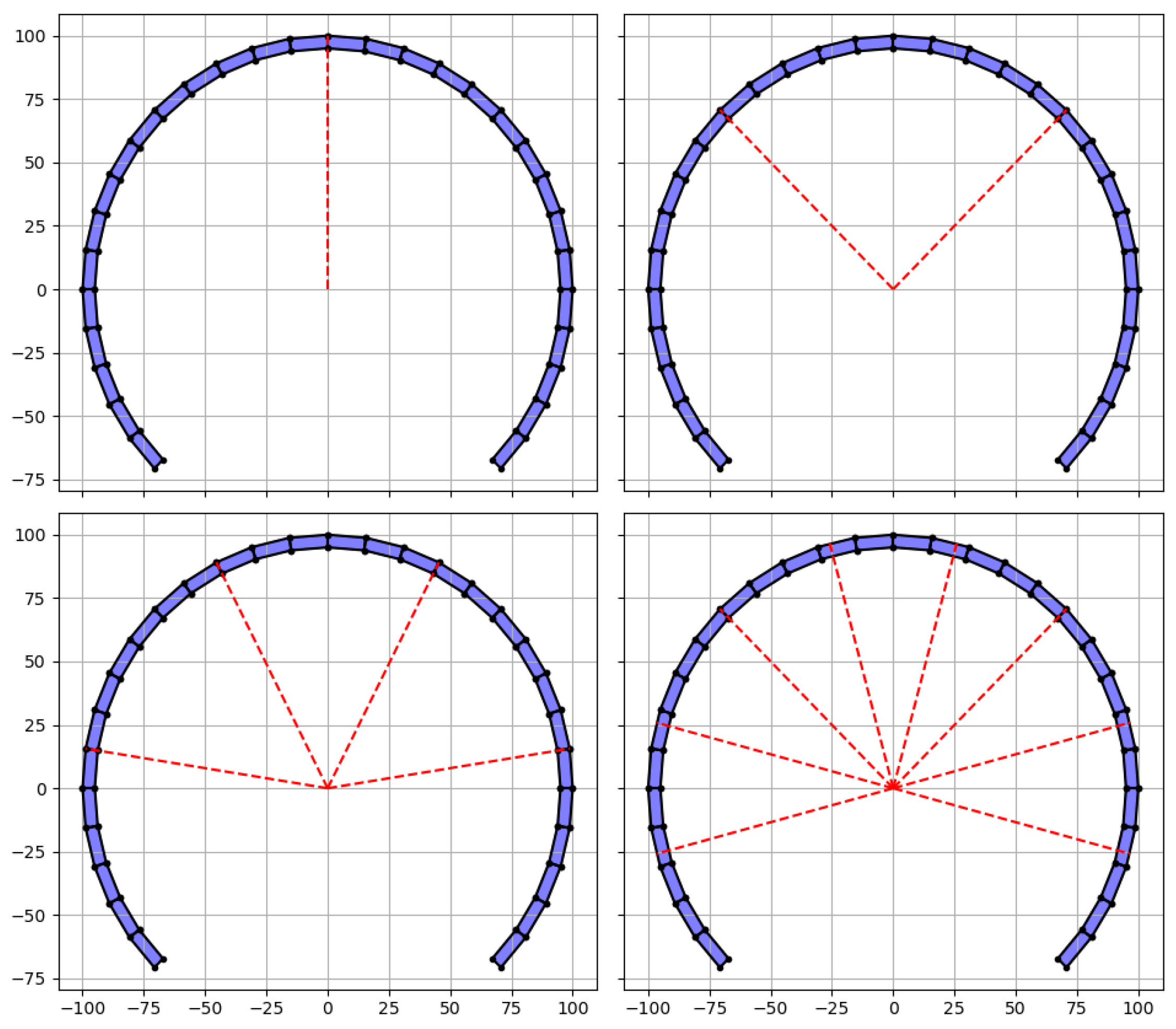
This structure is parameterized such that a vector of the design variables describes the radii of the structure at equidistant points along the circumference. A cubic spline is then fitted through these radii and the overall shape of a trial design is found. This is shown in Figure 6.

This parametrization scheme is selected, as the number of design variables can be systematically increased to investigate the performance of the surrogate models as a function of the dimensionality of the problem. The radii are sampled between 90 mm and 110 mm, and the accumulated arc length is limited to 2000 with the default arc length increment set to 100.

5. Results

The results of six different gradient-enhanced surrogate models are found. These include the domain-transformed versions for both the NSMs and STSMs, as well as their standard min-max implementations. NSMs include versions where the shape parameter of the surrogate models in the network is allowed to vary and where the parameter is kept constant for all the models in the network. By keeping the shape parameter constant, the NSM model has the same number of tunable parameters as the STSM. The number of tunable parameters for NSM and STSM is shown in

Table 1. The number of parameters that must be tuned in the NSM, where the shape parameter is kept constant, the shape parameter is allowed to vary, and the STSM. The number of parameters is expressed as a function of the number of centers K and the number of RBF models L in the NSM.

Parameters	NSM Constant Shape Parameter	NSM Varying Shape Parameter	STSM
Weights	K	K	K
Shape Parameters	1	L	1

. The models are constructed on an equal number of sampled points and are evaluated by comparing the predicted load-displacement paths to the actual results.

Initially, a simple univariate shape variable problem is completed using 7 designs sampled using LHS. Figure 7 compares the predicted load-displacement curves with the actual response for four random test designs.

The models are then assessed further by calculating the root mean square error (RMSE) for 75 load displacement paths for randomly sampled designs. The RMSE is calculated by comparing the approximated load ($\lambda$) and displacement (u) results of the model to the new 75 sampled load displacement paths. The models are evaluated at the arc length positions found by the solver for each of the new load displacement paths. This implies that the models must predict at new design variable locations as well as new arc length or pseudo-time locations. This RMSE for a single load-displacement curve is expressed as

$$RMSE=\sqrt{\frac{1}{n}\sum _i^n{({\lambda }_i^{approx}-{\lambda }_i^{target})}^2+\frac{1}{n}\sum _i^n{(u_i^{approx}-u_i^{target})}^2},$$

(13)

where n is the number of arc length steps and the values of $\lambda$, and u are normalized using the maximum values from the training samples.

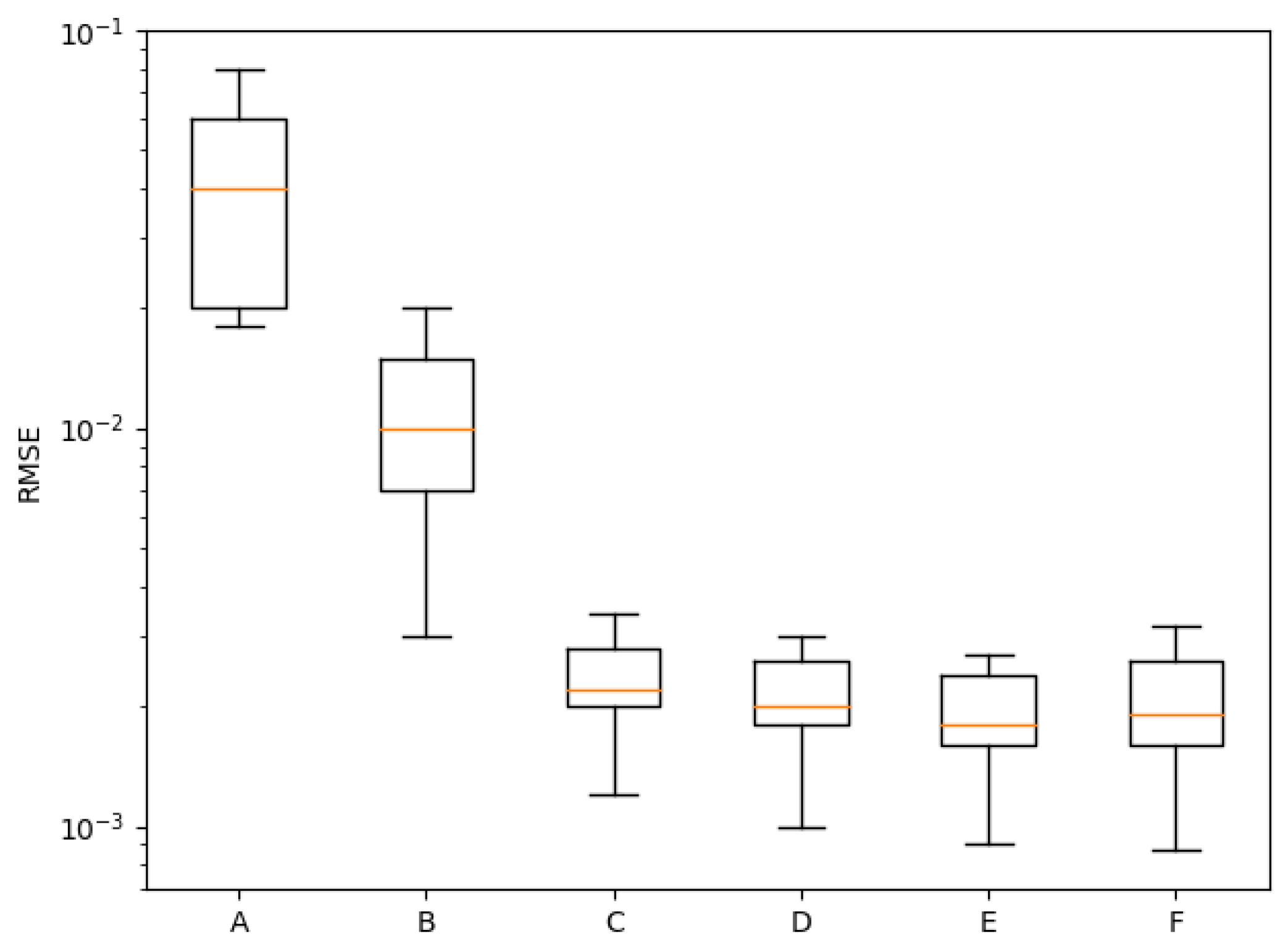
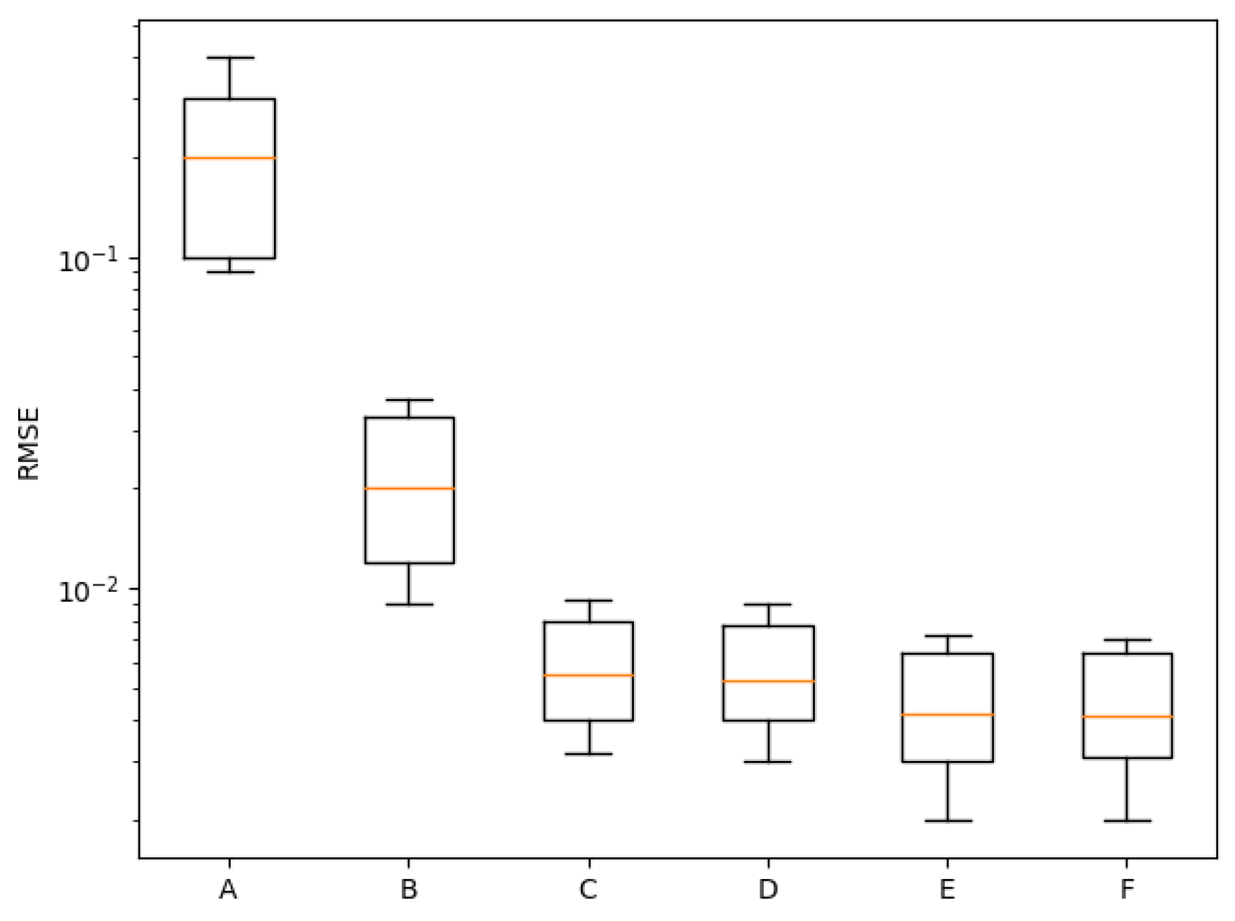
The average RMSE results are shown in Figure 8 in the form of a box and whisker plot.

Clearly, the NSM outperforms the STSM, but performing the gradient-based domain transformation offers a significant improvement to the predictive performance of the STSM. There is also very little improvement (if any) in the NSM when the shape parameter is allowed to vary compared to when the shape parameter is kept constant. Hence, the improved NSM fits are not the result of additional shape parameter flexibility but rather due to the ability of the NSM to complete different domain transformations as a function of the pseudo-time.

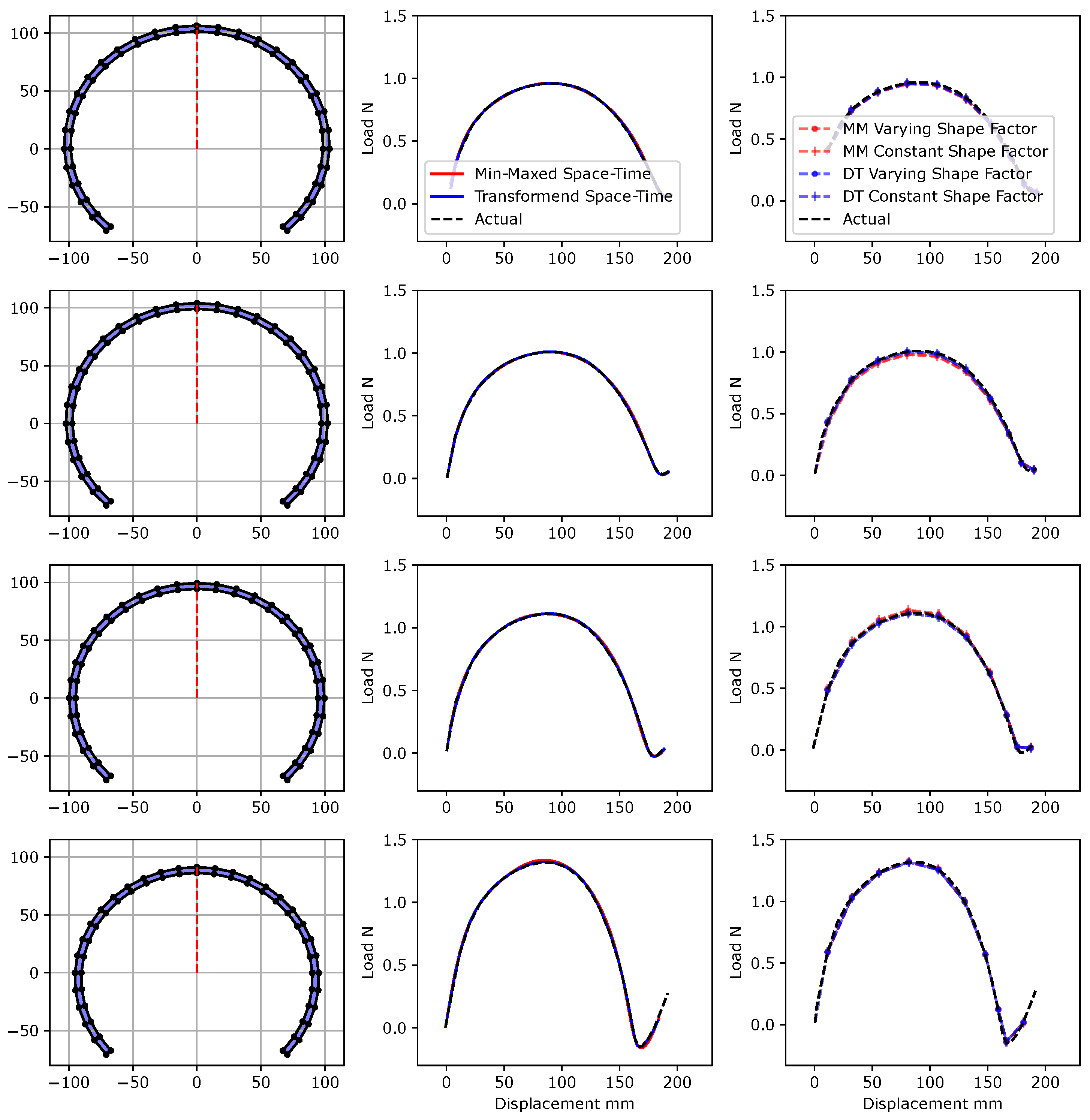
The dimensionality of the problem is now increased to two shape variables and the number of LHS samples is increased to 12. The results of the model are again overlaid with the simulated results in Figure 9, and the average RMSE results are displayed in Figure 10.

The results of the two-variable shape variable problem are similar to the univariate shape variable problem, with the NSMs outperforming the STSMs. In addition, the domain transformation improves both the NSMs and STSMs. The benefit of an appropriately transformed domain is evident for the two-variable problem. The difference in performance between the min-maxed models and the transformed models clearly increased, while there is a negligible difference between the varying shape parameters models compared to the constant shape parameter models.

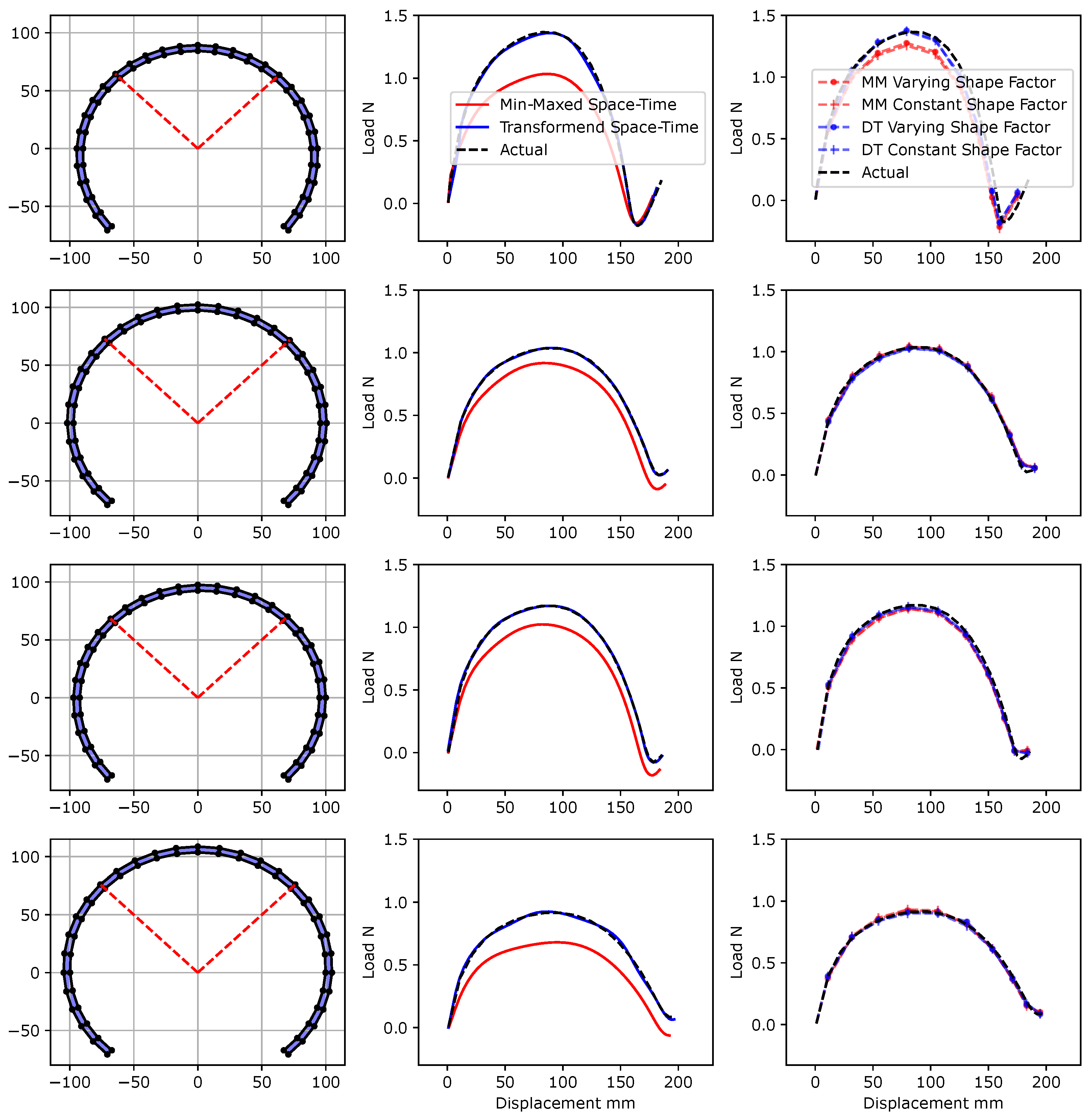
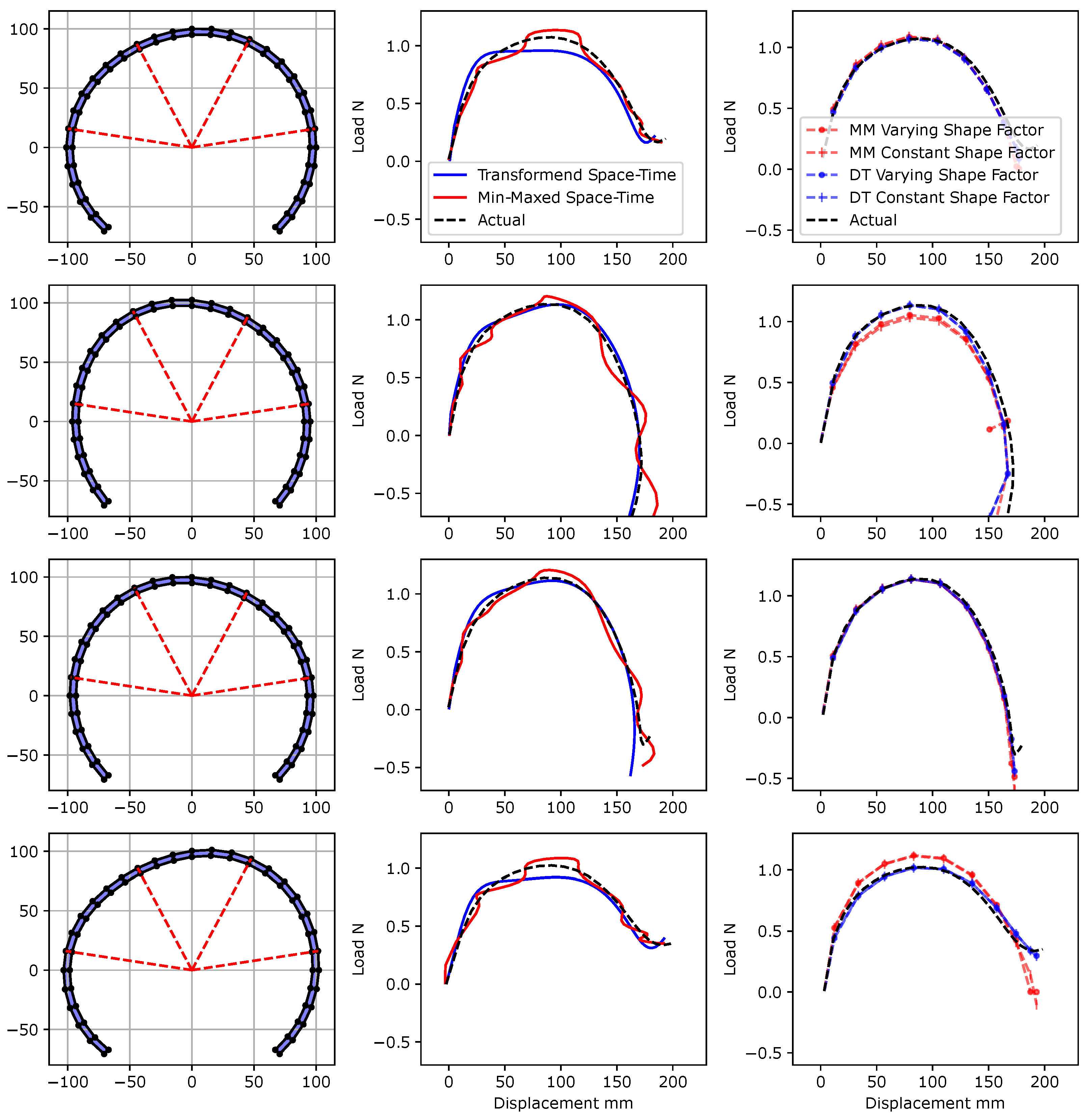
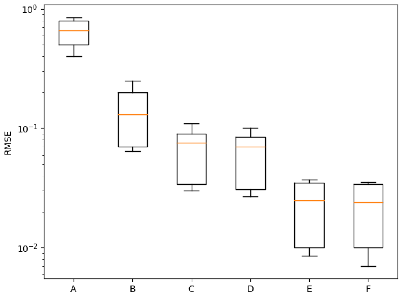
Lastly, the problem dimension and the LHS sample number are increased to 4 shape variables and 25 samples respectively. The results are presented in Figure 11 and Figure 12.

This problem demonstrates that the benefit of appropriately transforming the construction domain increases with the problem dimension. The min-max STSMs offer extremely poor predictions of the underlying function, while the transformed model remained robust.

The NSMs still outperform the STSMs, but there is a clear improvement with higher problem dimensions when the transformed domain is employed as compared to the min-max scaling. On the other hand, the varying shape parameter offers very little improvement to the model over the constant shape parameter models, despite this increase in flexibility.

6. Discussion and Conclusions

Constructing surrogate models to predict the spatio-temporal behavior of a system requires careful consideration as a naive implementation may be unable to capture the inherent complexities present in the spatio-temporal response. This study compares two strategies to construct spatio-temporal surrogates, namely, space-time surrogate models (STSMs) and network surrogate models (NSMs). From this, two main findings regarding the construction of surrogate models are observed.

Firstly, merely including gradient information in the construction of the surrogate models is not sufficient to construct high-quality models. Instead, the gradients should be employed to transform the domain to a more isotropic domain (the inherent assumption of RBFs). This enables the construction of accurate surrogate models for higher- dimensional problems.

Secondly, NSMs significantly outperform the STSMs. The results from the constant and varying shape parameter models demonstrate that this increase in performance is not due to the ability of the NSM to fit different shape parameters, but rather it is due to two underlying characteristics of the problem:

• The locations of the centers of the space-time RBF model have a non-uniform structure to them, i.e., the pseudo-time variable is sampled more densely than the shape variables.
• A single linear transformation might not be sufficient to transform the domain to be isotropic. The shape variables may impact the results differently at different stages in the pseudo-time variable domain and therefore a nonlinear transformation scheme that is a function of the pseudo-time variable is required.

References

- Nuñez, L.; Regis, R.G.; Varela, K. Accelerated Random Search for constrained global optimization assisted by Radial Basis Function surrogates. J. Comput. Appl. Math. 2018, 340, 276–295. [Google Scholar] [CrossRef]
- Ryu, Y.S.; Haririan, M.; Wu, C.C.; Arora, J.S. Structural design sensitivity analysis of nonlinear response. Comput. Struct. 1985, 21, 245–255. [Google Scholar] [CrossRef]
- Olhoff, N.; Lund, E. Finite Element Based Engineering Design Sensitivity Analysis and Optimization. Ph.D. Thesis, Aalborg University, Aalborg, Denmark, 1995. [Google Scholar] [CrossRef]
- Hisada, T. Recent Progress in Nonlinear FEM-Based Sensitivity Analysis. JSME Int. J. 1995, 38, 430–433. [Google Scholar] [CrossRef] [Green Version]
- Parente, J.; Vaz, L.E. On evaluation of shape sensitivities of non-linear critical loads. Int. J. Numer. Methods Eng. 2003, 56, 809–846. [Google Scholar] [CrossRef]
- Dhondt, G.; Wittig, K. CalculixX: A Free Software Three-Dimensional Structural Finite Element Program. 1998. Available online: http://www.calculix.de/ (accessed on 1 February 2023).
- Komkov, V.; Choi, K.K.; Haug, E.J.; Systems, F.d.S. Design sensitivity analysis of structural systems. Math. Sci. Eng. 1986, 177, 1–82. [Google Scholar] [CrossRef]
- Balagangadhar, D.; Roy, S. Design sensitivity analysis and optimization of steady fluid-thermal systems. Comput. Methods Appl. Mech. Eng. 2001, 190, 5465–5479. [Google Scholar] [CrossRef]
- Newman, J.C.; Taylor, A.C.; Barnwell, R.W.; Newman, P.A.; Hou, G.J.W. Overview of Sensitivity Analysis and Shape Optimization for Complex Aerodynamic Configurations. J. Aircr. 1999, 36, 87–96. [Google Scholar] [CrossRef] [Green Version]
- Laurent, L.; Le Riche, R.; Soulier, B.; Boucard, P.A. An Overview of Gradient-Enhanced Metamodels with Applications. Arch. Comput. Methods Eng. 2017, 26, 61–106. [Google Scholar] [CrossRef] [Green Version]
- Snyman, J.; Wilke, D. Practical Mathematical Optimization: Basic Optimization Theory and Gradient-Based Algorithms; Springer Optimization and Its Applications; Springer International Publishing: Berlin/Heidelberg, Germany, 2018. [Google Scholar]
- Urquhart, M.; Ljungskog, E.; Sebben, S. Surrogate-based optimisation using adaptively scaled radial basis functions. Appl. Soft Comput. J. 2020, 88, 106050. [Google Scholar] [CrossRef]
- Jones, D.R. A Taxonomy of Global Optimization Methods Based on Response Surfaces. J. Glob. Optim. 2001, 21, 345–383. [Google Scholar] [CrossRef]
- Viana, F.A.; Gogu, C.; Goel, T. Surrogate modeling: Tricks that endured the test of time and some recent developments. Struct. Multidiscip. Optim. 2021, 64, 2881–2908. [Google Scholar] [CrossRef]
- Bouhlel, M.A.; Martins, J.R. Gradient-enhanced kriging for high-dimensional problems. Eng. Comput. 2019, 35, 157–173. [Google Scholar] [CrossRef] [Green Version]
- Bogaert, P. Comparison of kriging techniques in a space-time context. Math. Geol. 1996, 28, 73–86. [Google Scholar] [CrossRef]
- Gao, F.L.; Bai, Y.C.; Lin, C.; Kim, I.Y. A time-space Kriging-based sequential metamodeling approach for multi-objective crashworthiness optimization. Appl. Math. Model. 2019, 69, 378–404. [Google Scholar] [CrossRef]
- Jang, J.; Lee, J.M.; Cho, S.G.; Kim, S.; Kim, J.M.; Hong, J.P.; Lee, T.H. Space-time kriging surrogate model to consider uncertainty of time interval of torque curve for electric power steering motor. IEEE Trans. Magn. 2018, 54, 8–11. [Google Scholar] [CrossRef]
- Kandroodi, M.R.; Araabi, B.N.; Bassiri, M.M.; Ahmadabadi, M.N. Estimation of Depth and Length of Defects from Magnetic Flux Leakage Measurements: Verification with Simulations, Experiments, and Pigging Data. IEEE Trans. Magn. 2017, 53, 6200310. [Google Scholar] [CrossRef]
- Ritto-Corrêa, M.; Camotim, D. On the arc-length and other quadratic control methods: Established, less known and new implementation procedures. Comput. Struct. 2008, 86, 1353–1368. [Google Scholar] [CrossRef]
- Bouwer, J.M.; Kok, S.; Wilke, D.N. Challenges and solutions to arc-length controlled structural shape design problems. Mech. Based Des. Struct. Mach. 2021, 1–32. [Google Scholar] [CrossRef]
- Koziel, S.; Ciaurri, D.E.; Leifsson, L. Surrogate-Based Methods. In Computational Optimization, Methods and Algorithms; Springer: Berlin/Heidelberg, Germany, 2011; pp. 33–59. [Google Scholar] [CrossRef]
- Vu Khac Ky, C.D. Surrogate-based methods for black-box optimization. Int. Trans. Oper. Res. 2019, 24, 393–424. [Google Scholar]
- Correia, D.; Wilke, D.N. Purposeful cross-validation: A novel cross-validation strategy for improved surrogate optimizability. Eng. Optim. 2021, 53, 1558–1573. [Google Scholar] [CrossRef]
- Bouwer, J.M.; Wilke, D.N.; Kok, S. A Novel and Fully Automated Domain Transformation Scheme for Near Optimal Surrogate Construction. arXiv 2023, arXiv:303.17694. [Google Scholar]
- White, D.A. Multiscale topology optimization using neural network surrogate models. Comput. Methods Appl. Mech. Eng. 2019, 346, 1118–1135. [Google Scholar] [CrossRef]
- Navaneeth, N.; Chakraborty, S. Surrogate assisted active subspace and active subspace assisted surrogate—A new paradigm for high dimensional structural reliability analysis. Comput. Methods Appl. Mech. Eng. 2022, 389, 114374. [Google Scholar] [CrossRef]
- Riks, E. The application of Newton’s method to the problem of elastic stability. J. Appl. Mech. Trans. ASME 1972, 39, 1060–1065. [Google Scholar] [CrossRef]
- DaDeppo, D.; Schmidt, E. Instability of Clamped-Hinged Circular Arches Subjected to a Point Load. Trans. Am. Soc. Mech. Eng. J. Appl. Mech. 1975, 42, 894–896. [Google Scholar] [CrossRef]
Figure 1.
An example of the LHS method in a two-dimensional problem with 7 and 12 samples, respectively.
Figure 2.
Locations of samples in a one and two design variable problem, respectively, with a pseudo-time variable t.
Figure 3.
An example of the NSM approximating an underlying function in blue. The solid black lines through the design variable domain indicate the constructed RBF models, while the dashed black lines through the pseudo-time domain indicate the interpolated final approximated curve.
Figure 4.
Example of an STSM overlaid with the underlying function. The STSM model is shown in red while the underlying function is in blue.
Figure 5.
The deformation of the deep semi-circular arch that is pinned at the left and clamped on right edge under a single point load. The point load in indicated with a red arrow, while the initial and final shape of the structure is denoted in blue and red respectively.
Figure 6.
The design variables of the deep semi-circular arch depicted in red with the design problem increasing in dimensionality.
Figure 7.
One shape variable problem results for four randomly generated designs. The simulated structures are shown of the left, followed by the STSM results, and then the NSM results with the labels MM and DT indicating min-maxed and full domain transformation, respectively.
Figure 8.
Average RMSE results for the one shape variable problem. (A) min-max STSM, (B) transformed STSM, (C) min-max NSM with a constant shape factor, (D) min-max NSM with a varying shape factor, (E) transformed NSM with a constant shape factor, and (F) transformed NSM with a varying shape factor.
Figure 9.
Two shape variables problem results for four randomly generated designs. The simulated structures are shown of the left, followed by the STSM results, and then the NSM results with the labels MM and DT indicating min-maxed and full domain transformation respectively.
Figure 10.
Average RMSE results for the two shape variable problem. (A) min-max STSM, (B) transformed STSM, (C) min-max NSM with a constant shape factor, (D) min-max NSM with a varying shape factor, (E) transformed NSM with a constant shape factor, and (F) transformed NSM with a varying shape factor.
Figure 11.
Four shape variable problem results for four randomly generated designs. The simulated structures are shown of the left, followed by the STSM results, and then the NSM results with the labels MM and DT indicated min-maxed and full domain transformation, respectively.
Figure 12.
Average RMSE results for the four shape variable problem. (A) min-max STSM, (B) transformed STSM, (C) min-max NSM with a constant shape factor, (D) min-max NSM with a varying shape factor, (E) transformed NSM with a constant shape factor, and (F) transformed NSM with a varying shape factor.