1. Introduction
We recall here the definition of curvature of a smooth curve. This is a fundamental concept in differential geometry that has been studied deeply in applied mathematics, engineering, and computer graphics. The problem of finding the curvature extremum has been investigated by many authors. We can point out some of their results on establishing necessary and sufficient conditions for the regularity of offset curves or tubular surfaces, designing various types of aesthetic curves from constrained conditions, representing and modifying curves to adapt principles of interpolation and animation, etc. In the following, we give a short description of the method for solving this problem and its limitations.
If
is the position vector of a smooth curve
, then the point
of
at
is written as a 3-tuple
, or a column vector
when used in a matrix expression; hence
is the row matrix
. The image of
or the map
itself is called a parametrization of
. Along
, we consider the coordinates of the Frenet frame
whose origin is located at points of
. From differential geometry and calculus (see [
1,
2]), we know that
where
and
are usually called the velocity vector and the acceleration vector of
at
t (or at
).
Let
be a parametrization of a smooth space curve
with
. Then, the curvature of
at
t is given by
where
,
, and
. Under this assumption, we usually find the maximum value of
on
by choosing the largest value of
at the points where
. However, how to solve the equation
exactly or approximately? In general, we cannot do it. Moreover, apart from this, the expression for
is complicated! Let us take
and write it out in the components of
. This gives
On the other hand, if
is the parametrization of
by the arc length
s, then from the relation
we obtain
This gives a simple expression for
:
However, we again encounter another hard problem: how to convert a parametrization of a smooth space curve by a general parameter t into the parametrization by the arc length s. In general, this is impossible.
To overcome those obstacles, many researchers restricted their attention to the class of Bézier curves and their variants. Recently, the papers related to maximizing or minimizing the curvature of these curves provided a lot of theoretical results and useful algorithms, as well as practical tools. We highlight some representative papers with a brief note. Ref. [
3] presents a unique design on a piecewise quadratic Bézier curve that interpolates its local maximum curvature points that are also its control points. Ref. [
4], adopted from [
3], proposes new methods to modify local curvature at the interpolation points by taking basis functions of higher degree. Ref. [
5] provides conditions for the curvature of a quadratic rational Bézier curve to be monotone or to have a local minimum and maximum. Ref. [
6] establishes conditions for Bézier plane curves generated by a matrix to have monotone curvature. Ref. [
7] also establishes conditions for Bézier curves to have monotone curvature, based on control points of the position vector of the curve and its derivatives. Ref. [
8] treats typical Bézier plane curves with one curvature extremum that can be easily calculated, which can help to divide the curve into two typical curves with monotone curvature.
Traditionally, the papers noted above and many others paid much attention to control points and polygons. Actually, these objects have direct effects on the shape of the curves, so they have been modified in order to obtain a curve with properties needed in design applications. However, we have some changes in mind when relating this widespread trend to our result in [
9]. The formula in [
9] (Theorem 3.1) can be seen as a way of approximation by interpolation with Bézier-spline curves. Therefore, we prefer to place emphasis on interpolated points. These points can be chosen in a way to design curves in
or
with desired shapes or can be taken from special partitions of the parameter interval of a smooth curve with given parametrization to approximate its curvature extremum.
Now, we go back to our main purpose: making a Maple procedure to compute the maximum value of the curvature. We restrict our attention to Bézier-spline curves. This objective is based on the power of Maple on symbolic computation and on solving polynomial equations of high degree and on the explicit piecewise cubic parametrization of these special curves.
The present paper is organized as follows. In
Section 2, we construct the Maple procedures to represent Bézier-spline space curves for both open and closed curves. In
Section 3, we propose a pseudo-algorithm for computing
, then we provide the full code of the procedures corresponding to the algorithm. In
Section 4, we discuss some modifications to obtain procedures to represent Bézier-spline plane curves and to compute their maximum curvature. In
Section 5, we give some concluding remarks.
2. Bézier-Spline Space Curves with Maple Parametrization
In this section, we consider a Bézier-spline curve, which is obtained from a closed-form solution to the inverse problem, which interpolates an ordered set of points
,
, …,
, given in [
9]. Such a plane curve can be obviously extended to a space curve
given by a piecewise cubic function
of
. According to the construction of such curves in [
9], we present here a more convenient way to derive their parametrization.
First,
is composed of the cubic functions
given by
where
and
, and
is the parametrization of the cubic Bézier curve
with the control points
,
,
, and
. These points satisfy the known relations
and
On the other hand, from [
9] (Theorem 3.1), the points
,
, are now in
with
and
, and for
, we have
where
(
) is evaluated by the formula
Finally, we can give a simple process to obtain a so-called
relaxed, uniform B-spline space curve that interpolates an ordered set of points
,
, …,
(see [
10]). The parametrization
of
is a piecewise cubic function on
whose components
,
, derived from (
2) and (
3), can be now given by
where
, and the
are obtained from (
5) for
, and
and
. Since
, the curvatures of
at
and
are both zero and we call
a
relaxed Bézier-spline space curve.
We are interested in the implementation of the above parametrization by a Maple procedure. We list here some Maple commands that will appear in our procedures. They are all very important and frequently used in graphic and computation programming:
args,
nargs,
op,
nops,
ERROR,
RETURN,
convert,
evalf,
diff,
expand,
floor,
for,
fsolve,
map,
max,
min,
piecewise,
plot,
plot3d,
proc,
seq,
solve,
unapply, and
while; in addition,
LinearAlgebra and
plots are the great packages containing many procedures for specific purposes. A declaration to create a function, e.g.,
f, such as
f:=x->F(x) or
f:=unapply(F(x),x) (sub-procedures in
F(x) are evaluated first), where
F(x) is an expression or a list of expressions in
x, is a very useful and convenient tool. In addition, the conditional structures
if-then-else and
if-then-elif-else are indispensable in branch programming, whereas the type “
list” is a flexible ordered arrangement of operands (or components, elements) inside the square brackets
[,
]. See [
11,
12] and Maple help pages in each session to know more details about meaning, syntax, and usage of these commands, structures, and types. The implementation of some specific task by calling a procedure name together with appropriate arguments is usually said to be a
calling sequence. As a convention, we choose type
list for elements of
or
.
Now, let us make a procedure to compute
on
from (
5)–(
7), with
and
. It takes
as its input and gives
as its output in the form of
such that
are the piecewise functions in
t on
. This procedure is called
BScurve3d and its full code is given in the following.
| BScurve3d |
| BScurve3d:=proc(Lst::list(list(realcons))) |
| local n,S,b,B,f,F,G,H,j,k; |
| n:=nops(Lst)-1: |
| for k from 0 to n do |
| S[k]:=Lst[k+1]: |
| end do: |
| for j from 0 to n-1 do |
| B[j]:=2^j*add(binomial(j+1,j-2*m)*(3/4)^m,m=0..floor(j/2)): |
| end do: |
| for k from 1 to n-1 do |
| b[k]:=(B[n-1-k]/B[n-1])*((-1)^k*S[0]+6*add((-1)^(k-j)*B[j-1]*S[j],j=1..k-1)) |
| +(B[k-1]/B[n-1])*((-1)^(n-k)*S[n]+6*add((-1)^(j-k)*B[n-1-j]*S[j],j=k..n-1)): |
| end do: |
| b[0]:=S[0]: |
| b[n]:=S[n]: |
| for k from 1 to n do |
| f[k]:=unapply(expand((k-t)^3*S[k-1]+(t-k+1)*(k-t)^2*(2*b[k-1]+b[k]) |
| +(t-k+1)^2*(k-t)*(b[k-1]+2*b[k])+(t-k+1)^3*S[k]),t): |
| end do: |
| F:=t->piecewise(-1<=t and t<1,f[1](t)[1], |
| seq([(k-1)<=t and t<k,f[k](t)[1]][],k=2..n-1),(n-1)<=t and t<n+1,f[n](t)[1]): |
| G:=t->piecewise(-1<=t and t<1,f[1](t)[2], |
| seq([(k-1)<=t and t<k,f[k](t)[2]][],k=2..n-1),(n-1)<=t and t<n+1,f[n](t)[2]): |
| H:=t->piecewise(-1<=t and t<1,f[1](t)[3], |
| seq([(k-1)<=t and t<k,f[k](t)[3]][],k=2..n-1),(n-1)<=t and t<n+1,f[n](t)[3]): |
| RETURN(unapply([F(t),G(t),H(t)],t)); |
| end proc: |
To declare a finite sequence of indexed expressions, we can use the operator
[ ] to extract the contents of a list. For example, the command
[][ ] results in
, and the declaration of the sequence
can be written as:
seq([k-1<=t and t<k,f[k](t)][],k=2..n-1). We have used this declaration in
BScurve3d.
If we have an ordered set of
distinct points in
that are declared in Maple as a list of lists
then we can obtain the position vector of the Bézier−spline curve
that interpolates these points by calling
f:=BScurve3d(S).The plot of
can be made by the procedure
spacecurve in the
plots
package with the command
The ‘
opts’ means
plotting options. To implement these steps, for instance, we set
and
. Then, the plot of the Bézier-spline curve
that interpolates
L is given by the calling sequence
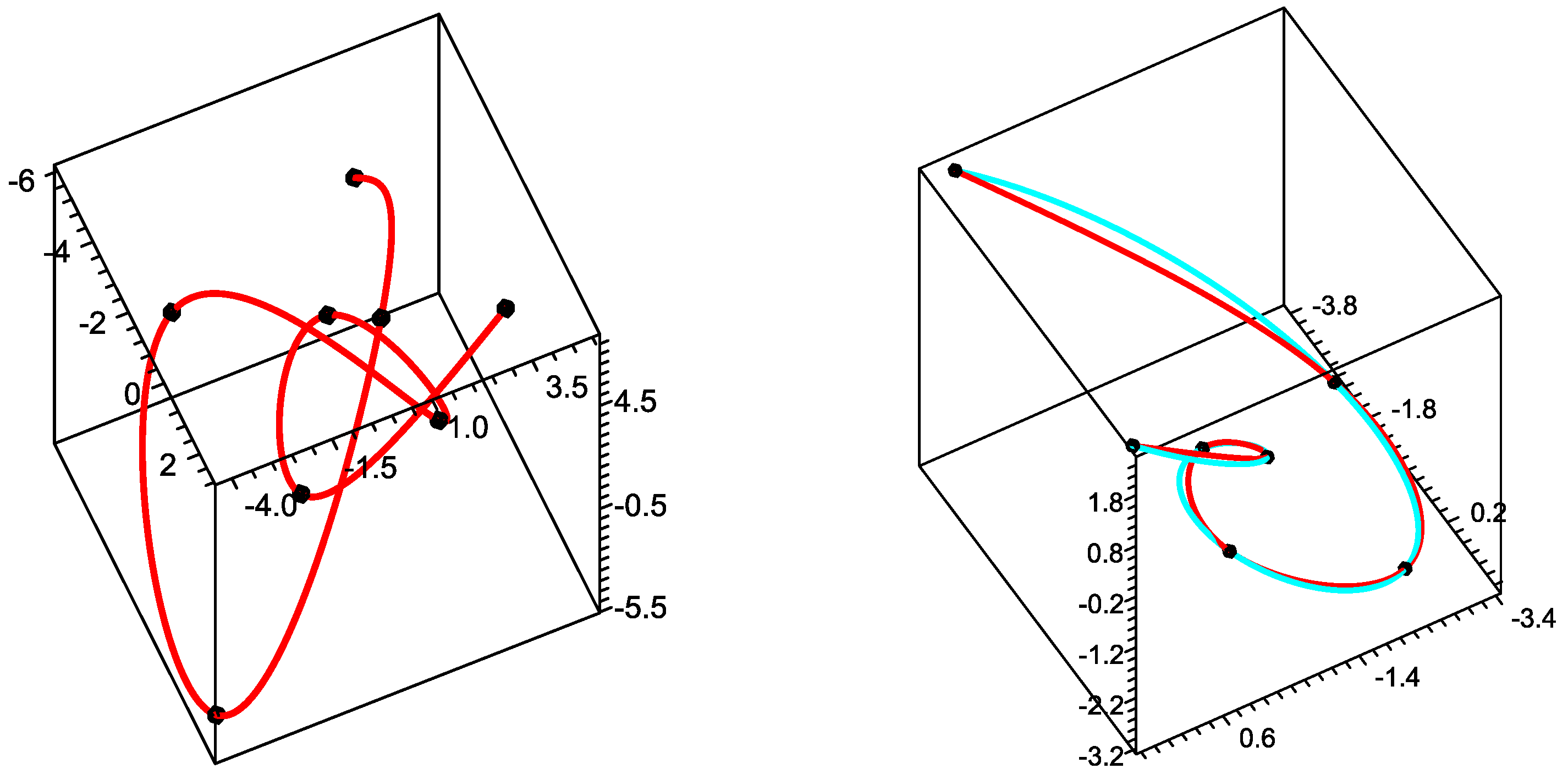
Figure 1 shows the curve
and the points of
L. We take one more example of interpolating an ordered set of points on a given space curve to see how well a Bézier-spline curve fits this curve. Let
be a curve whose parametrization is
,
, with the declaration
Consider a partition of
by the points
,
,
,
,
,
,
, and set
The curve
and its approximation by a Bézier-spline curve
are also given in
Figure 1.
We will make some changes to obtain a so-called
closed, uniform B-spline space curve that interpolates an ordered set of points
,
, …,
, with
(see [
10]). We call such a curve a
closed Bézier-spline space curve. In this case, we choose appropriate settings to have again the relations (
3) and (
4) at the common point. The first setting should be
. Then,
is still composed of the cubic Bézier curves
,
, as above. Specifically, at the interpolated point
, (
4) becomes
where we have from (
3) that
Now, from (
8) and (
9), we get the last setting
It is easy to have another Maple procedure, say
BScurve3dC, for representing a closed Bézier-spline space curve
from the dataset
with
, and the settings (
10) and
. From the above discussion, the parametrization
of
has the components
given by (
7), and we can check that
Therefore, is in again and have the same curvature at their common point.
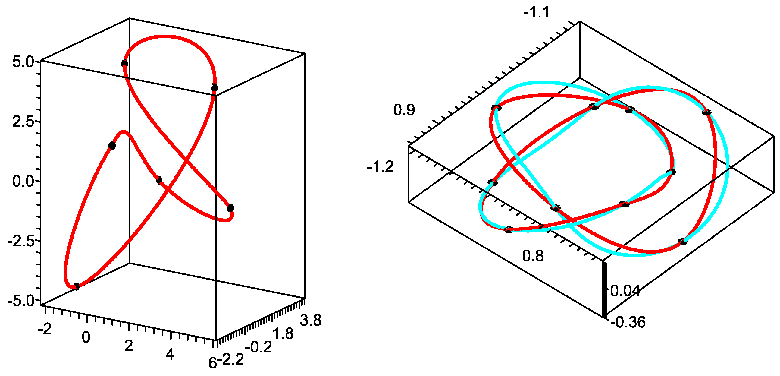
Let us take some examples on using
BScurve3dC. As the steps to display closed Bézier-spline space curves are the same as for
BScurve3d, we just give the graphical results of these examples. Note that the initial and terminal points of the input list for
BScurve3dC have to be the same. Let
L be the list
The display of the closed Bézier-spline curve
that interpolates
L is given in
Figure 2. Let
be the parametrization of a closed space curve
called a
trefoil knot (see [
1] (p. 897)) with
The endpoints of
coincide with the point
. Let
T be a set of points on
such that
In
Figure 2, we also give the display of
together with its approximation
that interpolates
T.
3. Computation of the Maximum Curvature of a Bézier-Spline Curve
Let
be a Bézier-spline curve that interpolates an ordered set
T of points
,
, …,
in
. Then
, the position vector of
, is a piecewise cubic function of
, given by its components
in (
7).
Avoiding the square root function, we have from (
1):
As
attains its maximum value on
only at solutions of the equation
or
in the intervals
and at their endpoints
, with
, we can find
on
by the procedure
MaxCurvature3d. However, at first, we present the procedure in the form of a pseudo-code algorithm. It would be easy to translate statements in such algorithms into Maple codes or other programming languages. Moreover, our discussion on how to use appropriate commands for a specific purpose will give a clear description of our procedures. In addition, we sometimes use built-in Maple procedures in those algorithms with their most simple form for convenience and simplicity.
Note that the left-hand side of (
11) is a polynomial of degree at most 7. Letting
Q be such a polynomial (in one variable, say,
t), we will use a powerful tool of Maple to find numerically all the zeros of
Q in a given interval. That is the procedure
fsolve and it has been called in Algorithm 1 by the command:
fsolve(Q,t,…). The output of this calling is a sequence of all real zeros of
Q in
. Moreover, the expressions of dot and cross products are given by the great package of Maple:
LinearAlgebra. We also select points in
at which
attains its maximum value. Thus, the output of Algorithm 1 consists of
and the set
in
. Now, for relaxed Bézier-spline curves, we give the full code of
MaxCurvature3d at the end of this section.
| Algorithm 1: Finding the maximum curvature of a Bézier-spline curve |
- Input:
a set T of points in ; - Output:
The maximum curvature of the Bézier-spline curve interpolating T; - 1:
; - 2:
forndo - 3:
, // from BScurve3d; - 4:
; - 5:
Q,t,i-1 .. i // Solving ( 11) for ; - 6:
; - 7:
// , ; - 8:
; - 9:
end for - 10:
; - 11:
; // on , on ; - 12:
return and ;
|
| MaxCurvature3d |
| MaxCurvature3d:=proc(L::list(list(realcons))) |
| local a,ad,A,AD,m,n,S,b,B,f,H,E,F,G,R,k,i,j,v,V,M,Kmax,N,P,Q,Sp,Tp,Tpoint; |
| n:=nops(L)-1: |
| for k from 0 to n do |
| S[k]:=L[k+1]: |
| end do: |
| for j from 0 to n-1 do |
| B[j]:=2^j*add(binomial(j+1,j-2*m)*(3/4)^m,m=0..floor(j/2)): |
| end do: |
| for k from 1 to n-1 do |
| b[k]:=(B[n-1-k]/B[n-1])*((-1)^k*S[0]+6*add((-1)^(k-j)*B[j-1]*S[j],j=1..k-1)) |
| +(B[k-1]/B[n-1])*((-1)^(n-k)*S[n]+6*add((-1)^(j-k)*B[n-1-j]*S[j],j=k..n-1)): |
| end do: |
| b[0]:=S[0]: |
| b[n]:=S[n]: |
| for k from 1 to n do |
| f[k]:=unapply(expand((k-t)^3*S[k-1]+(t-k+1)*(k-t)^2*(2*b[k-1]+b[k]) |
| +(t-k+1)^2*(k-t)*(b[k-1]+2*b[k])+(t-k+1)^3*S[k]),t): |
| end do: |
| Sp:={}: |
| for i from 1 to n do |
| v:=unapply(diff(f[i](t),t),t): |
| a:=unapply(diff(f[i](t),t$2),t): |
| ad:=unapply(diff(f[i](t),t$3),t): |
| V:=convert(v(t),Vector): |
| A:=convert(a(t),Vector): |
| AD:=convert(ad(t),Vector): |
| M:=expand(LinearAlgebra[DotProduct](V,V,conjugate=false)): |
| N:=expand(LinearAlgebra[DotProduct](V,A,conjugate=false)): |
| G:=map(expand,LinearAlgebra[CrossProduct](V,A)): |
| H:=LinearAlgebra[CrossProduct](V,AD): |
| E:=expand(LinearAlgebra[DotProduct](G,H,conjugate=false)): |
| R:=expand(LinearAlgebra[DotProduct](G,G,conjugate=false)): |
| Q:=expand(M*E-3*R*N): |
| F[i]:=unapply(sqrt(abs(R))/abs(M)^(3/2),t): |
| P:={fsolve(Q,t,i-1..i)}: |
| m[i]:=max(seq(F[i](P[j]),j=1..nops(P)),F[i](i-1),F[i](i)): |
| Sp:=Sp union P: |
| end do: |
| Kmax:=max(seq(m[j],j=1..n)): |
| Tpoint:={}: |
| for i from 1 to n do |
| if (abs(F[i](i-1)-Kmax)=0) or (abs(F[i](i-1)-Kmax)=0.) then |
| Tpoint:= Tpoint union {i-1}: |
| elif (abs(F[i](i)-Kmax)=0) or (abs(F[i](i)-Kmax)=0.) then |
| Tpoint:= Tpoint union {i}: |
| end if: |
| end do: |
| if nops(Sp)=0 then |
| RETURN(Kmax,Tpoint); |
| end if: |
| for j from 1 to nops(Sp) do |
| if (floor(Sp[j])=n) then |
| if (abs(F[n](Sp[j])-Kmax)=0 or abs(F[n](Sp[j])-Kmax)=0.) then |
| Tpoint:= Tpoint union {n}: |
| end if: |
| elif (abs(F[floor(Sp[j])+1](Sp[j])-Kmax)=0 or |
| abs(F[floor(Sp[j])+1](Sp[j])-Kmax)=0.) then |
| Tpoint:= Tpoint union {Sp[j]}: |
| end if: |
| end do: |
| RETURN(Kmax,Tpoint); |
| end proc: |
Here we give an explanation of how to determine the set . We first check whether i () belongs to this set, then we check the same for all solutions of the equation . In addition, when we need the value for a point , we should take an appropriate component of ; if , then we take , else we take , since .
We use
MaxCurvature3d to determine
in the examples whose graphical results are given in
Figure 1. From the lists
L and
in these examples, the calling sequences
MaxCurvature3d(
L) and
MaxCurvature3d() result in
respectively. If the parametrization of
is
, then
are the maximum curvature points on the curves
and
, respectively.
The new version of
MaxCurvature3d for closed Bézier-spline curves, say,
MaxCurvature3dC, can be derived easily from Algorithm 1 with the modification “
from
BScurve3dC”. Then, we use
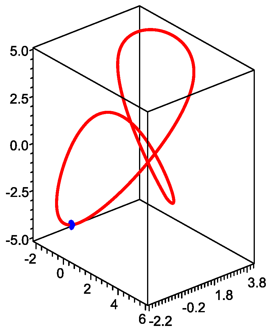
MaxCurvature3dC to find
of
displayed in
Figure 2 and we obtain the result
Let
be the parametrization of
. The point
is given in
Figure 3 and this maximum point of curvature of
is very close to the interpolated point
.
To avoid a comparison error between fractions and decimal numbers, we may use the decimal point ‘.’ for at least one component of the points in the list argument of MaxCurvature3d. Note that the result of fsolve only contains decimal numbers, so it will give us ‘’, for instance, if it contains the integer ‘2’. To cover this case, we add a condition such as ‘’ in the definition of MaxCurvature3d, and it should be sometimes ‘’ with some positive integer m when we need to obtain an expected result.
4. Remarks on the Two-Dimensional Case
For a relaxed Bézier-spline plane curve
that interpolates a dataset
M of points
,
, …,
in
, we have already a procedure to obtain its position vector
. That is just removing the lines
H:=t->⋯ and modifying the lines
RETURN(t->[F(t),G(t),H(t)]) to
RETURN(t->[F(t),G(t)]) in
BScurve3d, and the remaining part is for
BScurve2d, the Maple parametrization of
. Maple provides the
plot procedure to display plane curves with their parametrization
,
, by the declaration
Accordingly, we first set
(
M), then we call
to display
. Similarly, we get
BScurve2dC, the new version of
BScurve2d
for closed Bézier−spline plane curves, from
BScurve3dC.
MaxCurvature3d can be modified to use only sets of points in
and we call its new version
MaxCurvature2d. Let
be a smooth plane curve with parametrization
. From the formula
with arc length parameter
s, we can write
for a general parameter
t, where
We also consider
and derive the following equation from
:
This equation has the same role as (
11), so we can make a new version of
MaxCurvature3d, say,
MaxCurvature2d, following the steps in Algorithm 1 with some modification: there is no cross product in this version. The expression of the local variable
Q in the definition of
MaxCurvature2d is given by the left-hand side of (
12). Note that the function
in the pseudo-code algorithm of
MaxCurvature2d is now
In the definition of
MaxCurvature2d, the matrix
J is declared at right above
Sp:={} by
and, then, we set
U:=J.V inside the
for loop at right below.
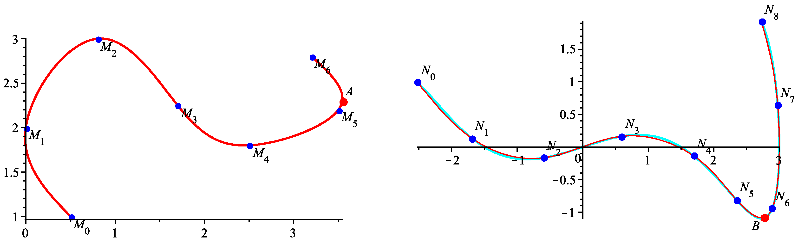
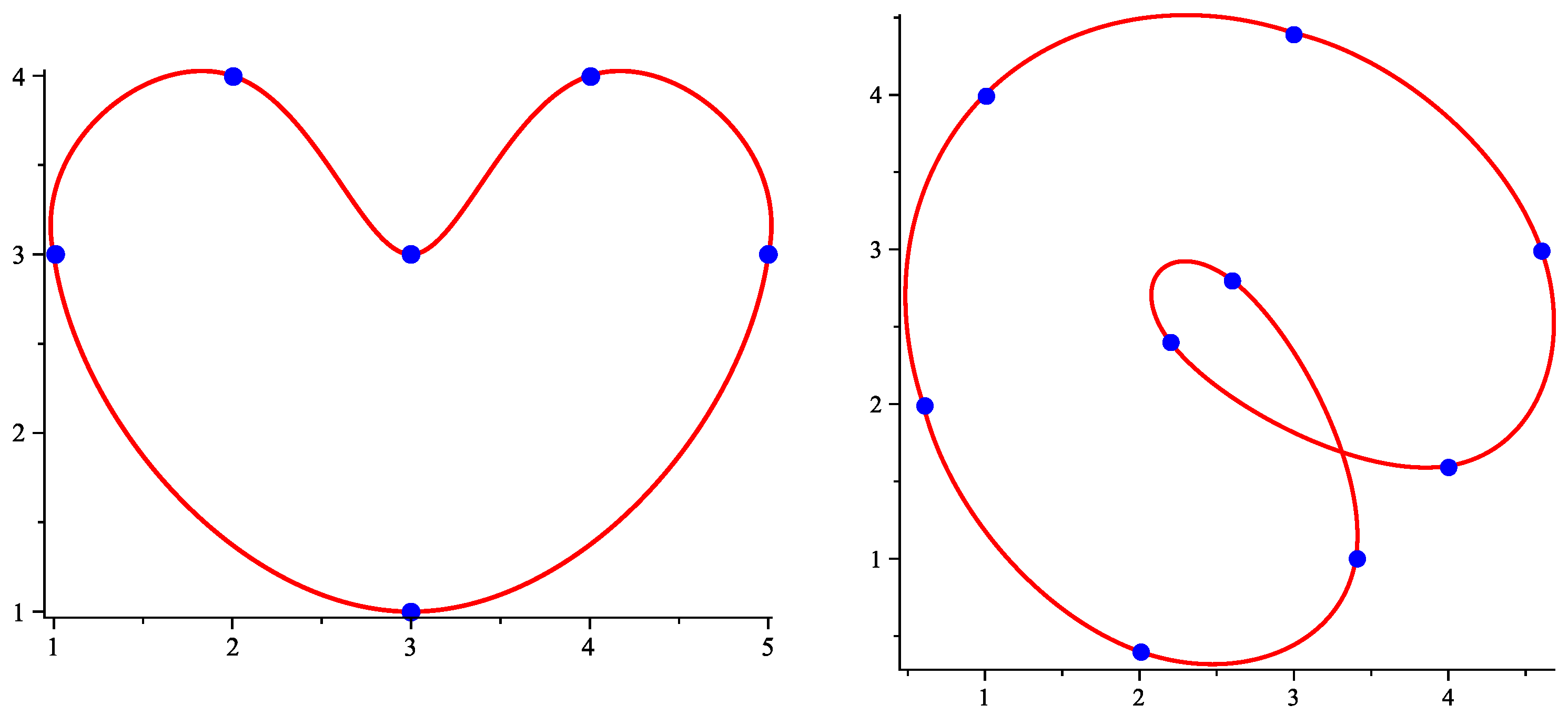
We give two more examples on getting the maximum curvature of a relaxed Bézier-spline plane curve and its maximum curvature points. Let
M be the list
and
be the Bézier-spline curve that interpolates
M. Then, we obtain the parametrization of
by setting
On the other hand, the calling sequence
MaxCurvature2d(M) gives us the result
Thus, the maximum curvature of is and this value is attained at the point .
Let
be a curve with the parametrization
,
, and let
be a partition of
. We set
. Letting
be the Bézier-spline curve that interpolates
N, we get its parametrization
Then, we derive
from the calling sequence
MaxCurvature2d(N). It follows that
attains the maximum curvature
at the point
.
The results from the two examples above are given in
Figure 4.
The next examples are dealing with closed Bézier-spline curves. The datasets
A and
B in the first two examples are chosen to be symmetric to an axis, namely
The curves
and
that interpolate
A and
B, respectively, are given in
Figure 5. The shapes of
and
can already be seen if we first display the interpolated points on the plane.
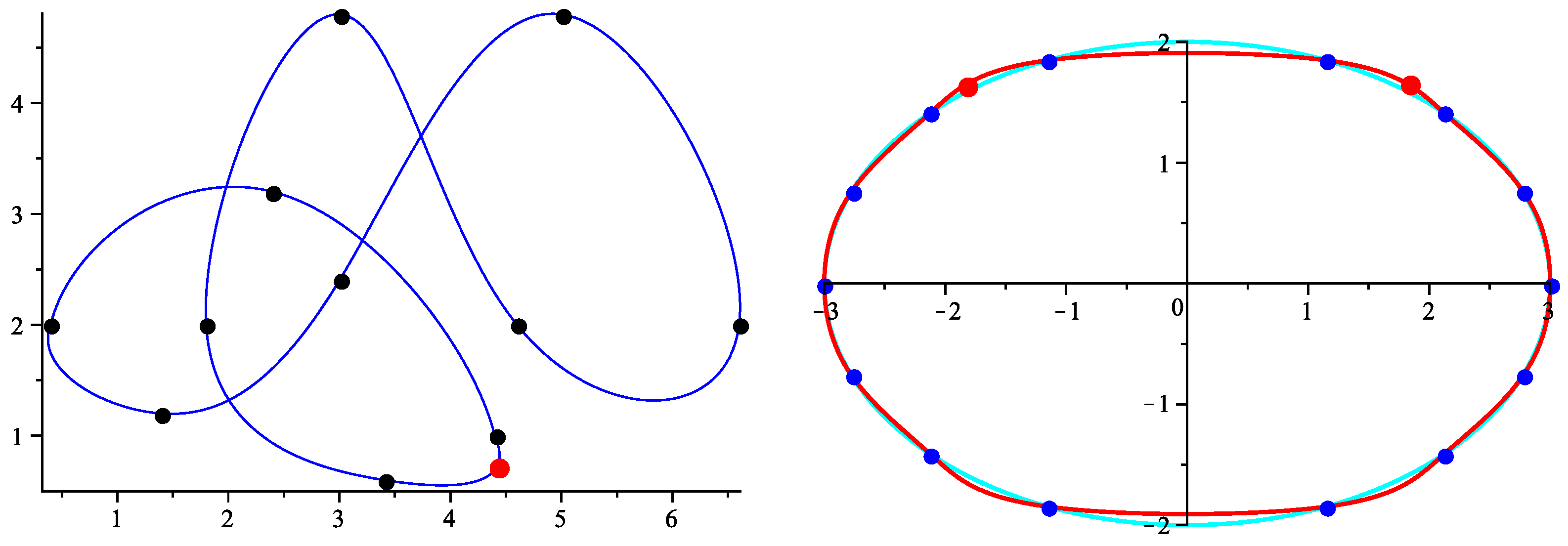
In the last two examples, we compute the maximum curvature of two closed Bézier-spline curves and show the maximum curvature points on these curves. The results are given in
Figure 6. The interpolated points (on the right) in
Figure 6 are chosen on the ellipse
(depicted in cyan).
We sometimes want to compute the curvature of a Bézier-spline curve at a
, so we should have a tool to do that. Algorithm 2 can be used to make such a tool.
| Algorithm 2: Finding the curvature of a Bézier-spline curve at its given point |
- Input:
a set T of points in , a point ; - Output:
The curvature at p of the Bézier-spline curve interpolating T; - 1:
ifthen - 2:
; - 3:
else - 4:
; - 5:
end if - 6:
, // from BScurve2d or BScurve2dC; - 7:
// ; - 8:
// , ; - 9;
return ;
|
It is easy to derive the Maple procedure from Algorithm 2 that we call Curvature2d or Curvature2dC, depending on whether is from BScurve2d or from BScurve2dC. Similarly, the extension of this procedure for the three-dimensional case can be obtained with the curvature function from Algorithm 1.


