1. Introduction
Atomization is a complex physical process, often considered from a multiphase perspective, which involves the breaking of a bulk fluid structure into fine droplets to increase the fluid’s surface area. This is a critical process in various engineering technologies with applications in fire suppression systems, paint technologies, agriculture, and fuel combustion. In these applications, the atomizer nozzle design significantly impacts the spray patterns. This, in turn, has a direct effect on the operational efficiency of these solutions. With atomization physics being highly non-linear, the development of numerical methods suitable for the prediction of atomization processes has attracted significant interest.
Atomization has been explored in various contexts from high-fidelity Eulerian methods [
1,
2,
3,
4] to more computationally tractable under-resolved hybrid Eulerian–Lagrangian [
5,
6,
7,
8] or purely Lagrangian [
9,
10,
11] approaches. High-fidelity Eulerian methods are attractive in research environments due to their ability to resolv flow from first principles [
4]; however, the high computational cost generally makes these approaches infeasible for industrial applications. Hybrid methods address this shortcoming by generating Lagrangian particles once fluid volumes cannot be resolved by the Eulerian grid. Unfortunately, either the droplet sizes are mesh-dependent [
5,
6,
8], or this generation step is model-dependent [
7]. These particles are generally treated as hard spheres with two-way coupling with the Eulerian fluid through drag models [
12]. Lagrangian methods are an interesting addition as they do not need to incorporate any particle generation. Rather, Lagrangian particles may simply flow away from the main fluid body. This circumvents any particle generation model; however, it does imply that droplets below the Lagrangian particle size cannot be resolved. While various numerical methods have been proposed for atomization, all these methods suffer from an additional problem that stems from the inherently multi-scale nature of the atomized fluid. That is to say that the raw data produced by these approaches are typically not suitable for quantitative comparison without additional post-processing. This is especially significant at the primary atomization level where large-scale multiphase fluid structures still exists.
Typically, atomization is quantified by the droplet Sauter mean diameter (SMD) distribution. While this is simple to evaluate for small droplets tracked with sub-grid methods [
6], if Eulerian–Lagrangian methods sample a distribution when generating the Lagrangian fluid droplets [
7], then this distribution must be known beforehand. Furthermore, as discussed by Li et al. [
4], this is not suitable when a larger fluid structure separates from the main body but is still ultimately resolved by the fluid grid. The solution proposed was to evaluate the SMD of these fluid structures directly. However, this requires the resolution of both the surface area and volume of the fluid structure, which is especially challenging for Lagrangian solvers. In the work of Holz et al. [
10], smoothed particle hydrodynamics (SPH) was used to simulate an atomization process in 2D. The flow was quantified by utilizing a connected component labeling algorithm to evaluate the geometrical properties of a large fluid ligament as well as to identify droplets formed by clusters of SPH particles. While this was able to treat fine droplets and larger fluid structures, this method was specifically crafted for the investigated case where it was known that only a single large-scale fluid body was present. Furthermore, additional work is required to generalize this technique to 3D space. Connected component labeling is also suitable for Eulerian methods such as the direct numerical simulation (DNS) of [
13], where this approach was used to identify individual droplets. The simulation made use of a two-phase flow model utilizing a smoothing parameter that allowed the appropriate cells to be flagged for the droplet surface and volume approximations. While suitable for high-fidelity data, connected component labeling is challenging to apply to low-fidelity simulation due to smoothing parameters being more diffuse, which in turn leads to less robust interface identification. Besides droplet SMD, liquid core characteristics are also of interest. In the work of Agarwal and Trujillo [
14], both the liquid core surface area and the average length were used to compare different atomization results. The length was determined in a conceptually similar fashion to [
10] where the maximum length of the connected fluid body was measured. The surface area measured was obtained by estimating the interface surface distance from the center of the domain as a function of a sweeping angle and temporally and spatially averaging this over the fluid core’s length.
These post-processing methods become application-specific due to them operating immediately on low-level spatial data. A sensible alternative comes from image processing since it is subject to similar multi-scale challenges. Specifically, the 2D fast Fourier transform
(FFT) is commonly employed in image processing to highlight dominant trends in the spatial distribution of image data. While traditional image processing typically uses this information for filtering and compression [
15], differences over the frequency spectrum can be used for robust multi-scale comparisons between images with complex structures [
16,
17].
Using image processing techniques are attractive from a verification perspective as well. Since atomization typically deals with high-speed dynamics that are sensitive to operating conditions, it is typical to quantify atomization using non-invasive techniques such as phase Doppler interferometry [
18,
19] or image processing techniques [
20,
21,
22]. In contrast to phase Doppler interferometry, which gives a direct measurement of droplet characteristics, imaging methods must make use of additional post-processing techniques to resolve droplet surface and volume information in a manner similar to numerical methods. As with numerical cases, application-specific methods can be developed for operating conditions that are fixed. An example of this can be seen in [
21] where well-defined image features specific to the application are used to generate heuristics used to evaluate stream properties. Besides direct image generation, as proposed in the work of [
23,
24], correlations between the X-ray scattering absorption measurement ratio and droplet shape can be used to determine the SMD of the droplet size distribution in a more abstract and generalizable manner. However, as with Doppler interferometry, this approach cannot be directly applied to numerical results.
This work proposes a post-processing scheme for primary atomization that forgoes directly processing spatial features and rather generates abstract but generalizable measures of the multiphase interface. Rather than focusing on extracting specific flow features from images, spectral data correlated to droplet size information will be generated and compared directly. The post-processing scheme strongly relies on multiphase information for surface identification similar to [
13]; however, this is now applied in a Lagrangian context. Furthermore, instead of using the multiphase interface to identify boundaries for a connected component labeling algorithm, the surface information itself is processed. This alleviates the need for sharp interfaces obtained from high-fidelity simulations and allows for low-fidelity simulations to also make use of this method. The scheme relies on the so-called color function of the continuous surface force (CSF) multiphase scheme [
25]. To demonstrate the workings of this scheme, a low-fidelity 3D simulation of the primary atomization of a viscous liquid via gas injection is performed for two different nozzle geometries using a meshless Lagrangian approach based on the generalized finite difference
(GFD) differential operators [
26,
27,
28]. The nozzles are quantitatively compared with the proposed scheme.
2. Materials and Methods
With the focus of this work being on post-processing techniques for primary atomization, low-fidelity simulations are considered to limit the computational cost of the study. Furthermore, droplets below the scale of the numerical GFD particles are not considered. As such, the simulations presented in this work only resolve the multiphase fluid mixture. The continuum considered in this work evolves according to the Navier–Stokes equations (NSE) for incompressible multiphase flow:
with
the velocity,
the density,
p the pressure,
the interface surface tension force and
a Newtonian shear stress tensor, with
the dynamic viscosity and:
the symmetric strain rate tensor for incompressible flow where ⊗ indicates the tensor product. It should be noted that gravity and other body forces are not considered in this work.
The GFD differential operators are used to discretize the equations of motion. The surface tension effects are resolved using the CSF model. This choice is fundamental to this work since the CSF model introduces an additional continuum field that is critical to the proposed post-processing scheme.
2.1. Simulation Method
This section provides a high-level overview of the numerical methods used to simulate the fluid system. The core goal is to provide context for the post-processing scheme. As such, the discussion focuses on the multiphase CSF model. For a complete description of the numerical method, readers are referred to [
29,
30].
2.1.1. Incompressible Generalized Finite Difference Method
A truly incompressible scheme similar to incompressible SPH (ISPH) [
31] is used to simulate the fluids. Specifically, a predictor step incorporating momentum diffusion and body forces of (
2) is used to obtain an intermediate velocity field
: The incompressibility condition of (
1) is enforced by projecting
onto a divergence-free space via the pressure gradient.
The discretized predictor update for the
th time-step is resolved as:
with
the time-step size,
the kinematic viscosity,
a dampening term for high-density ratio systems [
30], and
the particle acceleration due to surface tension. The subscript
i denotes information associated with the
ith particle, and
indicates the GFD discretization of the differential operator [
26,
27,
28]. The differential operators acting on the velocity field are resolved as:
with
the dimension,
the relative displacement of particle
i from
j, and
I the indexing set of particle
i’s neighbors:
which are the truncation tensor and offset vector, respectively, and
is a quintic kernel function [
32]:
with support radius
. Since
exploits information from the multiphase scheme, it is discussed in
Section 2.1.2 alongside
.
The dampening term is resolved as:
with
the velocity difference between particle
i and
j projected onto
and:
with
a user-specified parameter to control the aggressiveness of the dampening.
The updated pressure is resolved by solving the discretized pressure Poisson equation (PPE):
with the velocity divergence:
and the pressure Laplacian:
where
is the average density. This discretization results in a large linear system that must be inverted. As presented in [
30], the biconjugate gradient stabilized (BiCGSTAB) method with a Jacobi pre-conditioner is used to solve this system.
To enforce the divergence-free condition:
with:
2.1.2. Multiphase Flow
The CSF method introduces a scalar color field
C that is used to distinguish fluid phases. With this information inherently Lagrangian, the color function is typically a constant particle property. To smooth out violent mixing at interfaces, a Shepard filter is applied to the color function:
where
is the indexing set of all particles in the first phase and in the support radius of the i
th particle. A particle completely submerged in the first phase is described by
, while
indicates a particle submerged in the second phase. Any other value indicates a particle in the support region of the multiphase interface. Material properties are resolved using the color function, with the particle density and viscosity being determined as:
with superscripts 0 and 1 indicating the material properties of the first and second fluids, respectively.
The surface tension resolution is based on the gradient of the color function. The normal direction
is resolved as:
As proposed by Yang et al. [
33], filtering based on the color gradient’s magnitude is applied to obtain the indexing set of interface particles:
where
N is the total number of particles and
is a user-specified parameter to control the aggressiveness of the filter. Setting
was found suitable for all simulations in this work. For all
, the interface normal is defined as
. The surface curvature
is resolved for any interface particle as the divergence of the surface normal:
It should be noted that only interface particles participate in this construction.
The acceleration due to the surface tension force is then resolved as:
with
the surface tension coefficient.
When considering (
19), the color gradient can be reused to obtain the viscosity gradient as:
2.2. Post-Processing
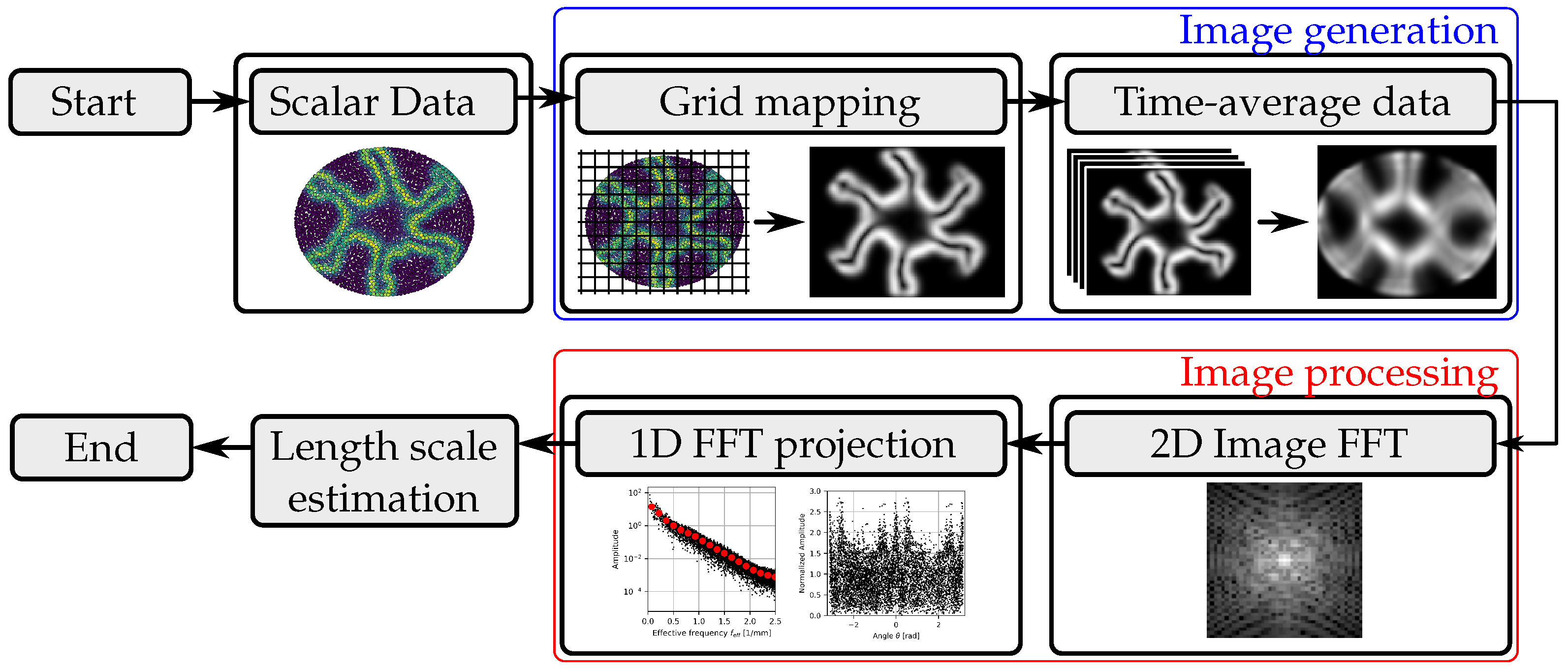
The post-processing applied in this work revolves around a two-step process, as shown in
Figure 1. The first step generates an image for further post-processing. The generated image represents a scalar continuum field evaluated on a regular-spaced grid that serves as the pixel intensity of the image. This is followed by applying a FFT on the image. The 2D spectral data are projected onto a 1D domain, which is then used for quantitative comparisons between numerical solutions.
This section is split into two parts, with the first describing of the image generation scheme and the second describing the spectral analysis procedure along with the interpretation of its output.
2.2.1. Image Generation
As a particle method is employed to simulate the fluid system, continuum fields are not readily available and must be constructed from a weighting process. A regularly spaced grid is generated over the domain of interest. In this work, this was at the outlet of the nozzle.
Since atomization is resolved from multiphase information, it is natural that the color field contains relevant information regarding this process. However, the color field provides information at the fluid volume level. Due to the low-fidelity simulations used in this work, relatively few small-scale fluid structures are generated. Furthermore, since a time-averaging approach is used, any droplets that are generated do not significantly perturb the image intensity. To circumvent these issues, an alternative measure based on surface information is proposed for this work. The argument for this is based on the idea that atomization takes place at fluid interfaces, and so, with an increase in interface area, more droplets are expected to form [
7]. Although these interfaces also evolve, as they are persistent large-scale structures, they sweep out regions that serve as droplet sources. Therefore, rather than focusing on the color field itself, the image generation process operates primarily on the color gradient magnitude.
Instantaneous snapshots are generated over regular time intervals
. These snapshots are used to generate the pixel grey-scale color intensity. For
at pixel
, the intensity
is obtained by applying a Shepard filter at the pixel’s corresponding point in the simulation space:
where
is the corresponding 3D position of pixel
,
is the grid spacing,
is the grid origin, and
is the indexing set of fluid particles within the support radius of
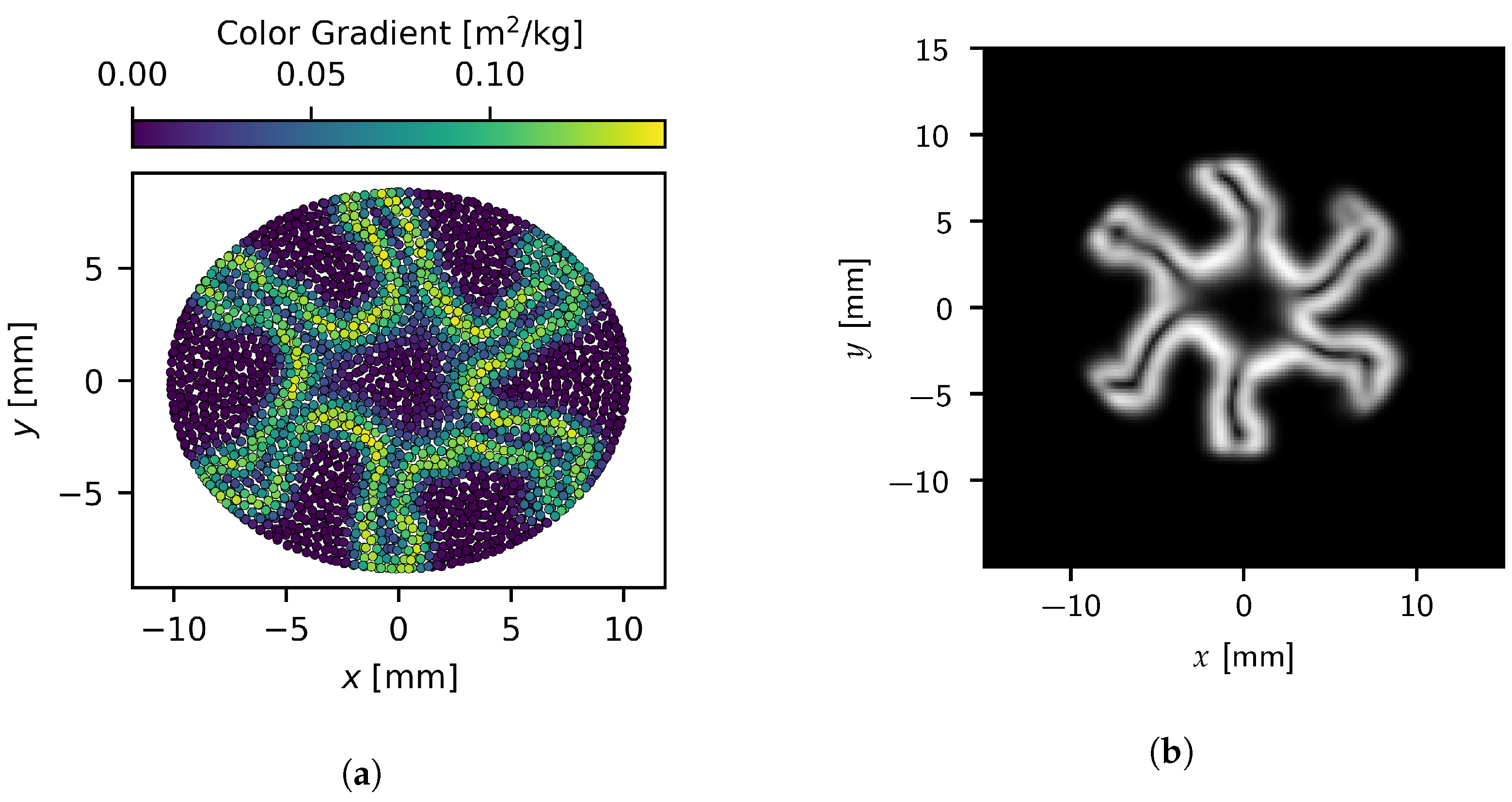
. Of course, the color gradient magnitude can be swapped for any other scalar field as well, with this work also considering density results. An example of the raw particle data as well as the instantaneous snapshot generated from these data is shown in
Figure 2a,b, respectively.
Finally, a single image is generated as the average of all instantaneous snapshots:
where
and
are the first and last snapshots considered, respectively. For all results presented in this work, a total of 200 snapshots are used for each image.
2.2.2. Image Processing
Once an image
F has been generated, the post-processing step follows by applying an FFT to the data. This produces a dual image of the outlet conditions in the frequency space:
with
the resolution of
F and
indicating the complex norm.
Since image
F was described over the simulation space, entries of the dual image are over the spatial frequency space. It should be mentioned that in the presented results, the DC offset at
in (
27) is shifted to the image center. Thus, for an image
F with resolution
over the domain:
equivalently represents the data over the domain:
with
the spatial sampling frequency, and
and
the x- and y-frequency, respectively.
As discussed in
Section 3,
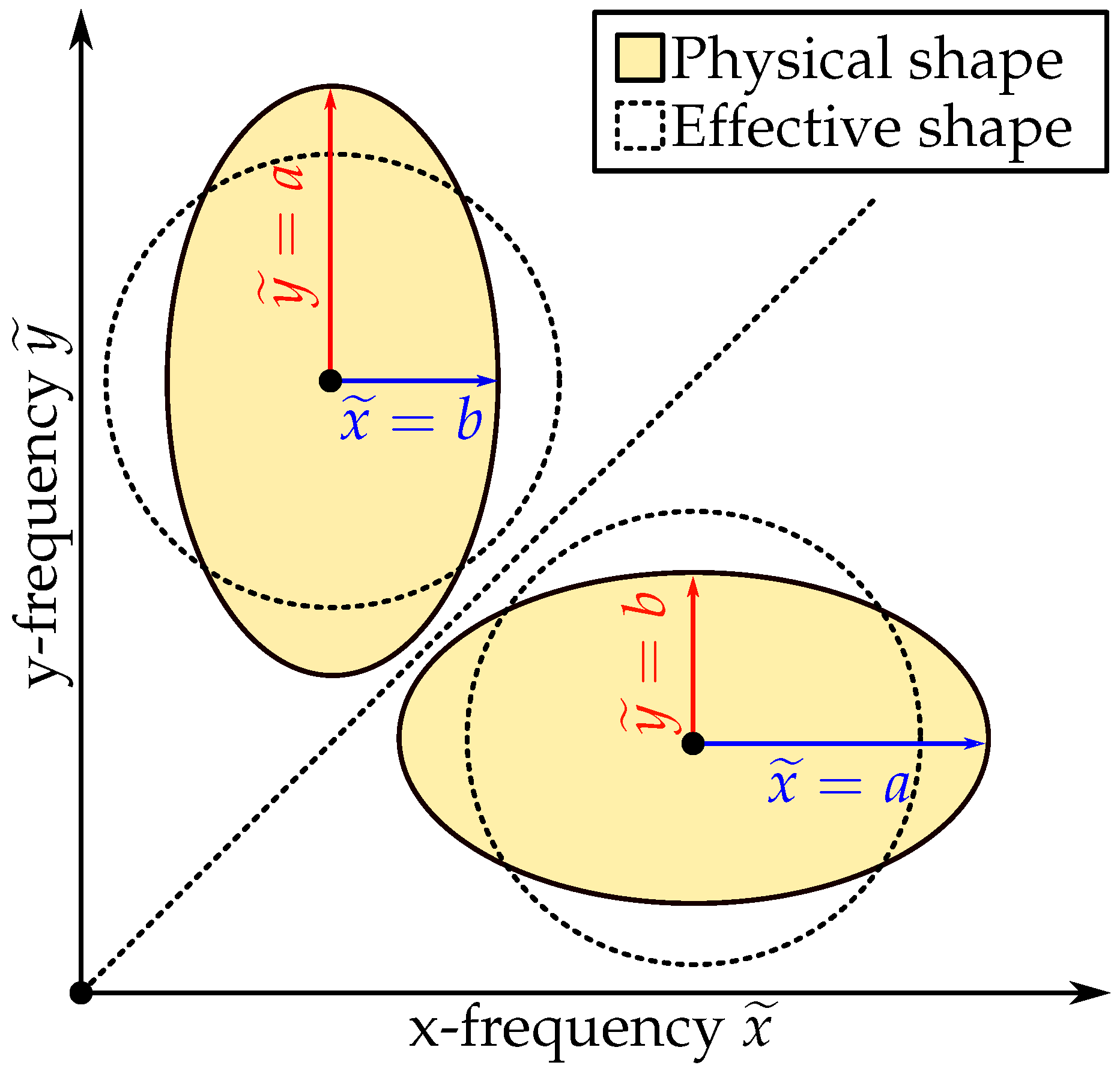
already highlights dominant structures in the spatial field; however, the dimensionality of the data can still be reduced when quantifying atomization. Ultimately, only the relative size is of interest for evaluating the feature sizes of the outlet interface.
Figure 3 highlights the problem with the 2D FFT data, where an arbitrary choice of coordinate system creates distinctions between particles of similar size. For each pixel, the anisotropic feature is transformed into an equivalently sized isotropic feature. This is achieved by determining an effective frequency
for each pixel based on the x- and y-frequency:
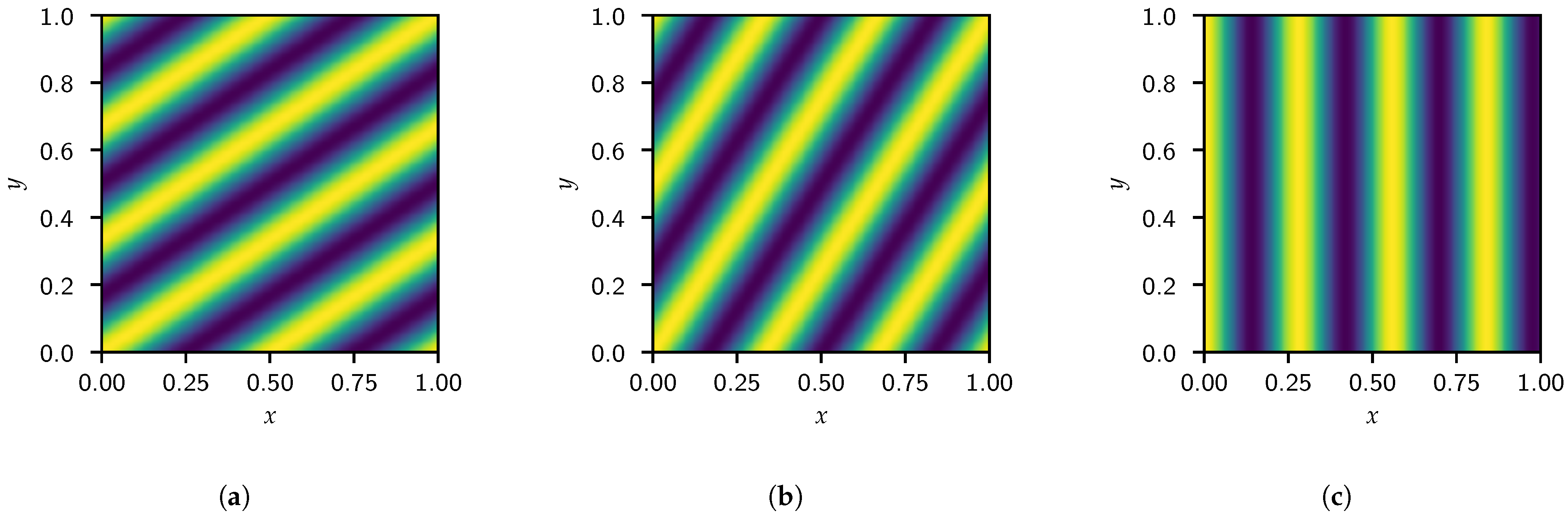
The effect of this transformation can be seen in
Figure 4 where the real component of the complex exponential
is plotted over a unit square for three different x- and y-frequencies that result in the same effective frequency. The length scales for all examples are equivalent, while the ratio between x- and y-frequencies determines the direction of these features. This implies that the dimensionality reduction results in the loss of information relating to the orientation of fluid structures.
To address this, along with the effective frequency projection, an additional 1D projection is constructed following the procedure proposed in [
17]. The FFT data are projected onto a 1D space based on the angle a pixel makes with the image center. Since length scale information is mixed in this projection, the FFT data are normalized based on their radial distance. Concentric circles are generated in frequency space. Any pixel falling in a band between two concentric circles is flagged as being part of that band. Each pixel’s data in the band are normalized by the mean of all pixel data in the band. This highlights angles that dominate the response over all length scales, and so, provides a measure for orientation and aspect ratios of fluid structures.
To compare results over , a final binning operation averages for all entries with frequencies in the bin range. This creates a low-dimensional quantifiable representation of the outlet data. This allows for clear comparison between structures over the system length scale ranging from a measure of the total information content, which directly relates to the total interface information, up to the GFD particle length scale and provides information about individual particles separating from the main fluid body. This averaging operation also allows for images of different resolutions to be compared against each other.
The machinery behind the image processing step is trivial as it only involves applying a standard FFT on the image data. By deconstructing the field data into weighted sinusoidal terms, the frequency of these waves provides a length scale for their associated information. That is to say that the FFT separates information content based on its distribution over length scales. This is what makes this approach attractive for design and optimization, as it is computationally inexpensive while still capturing information over system length scales.
It is important to note that this approach does not generate a distribution of the droplet SMD. However, as this scheme operates on an image of the multiphase interface, experimental work that produces images of atomization patterns can be used as inputs to this scheme to generate data for validation or correlations to the outputs of other higher-level processes.
3. Results and Discussion
This section is separated into two main results. The first part deals with a verification study of the post-processing scheme. The second part applies the proposed scheme to the outputs obtained from low-fidelity atomization results to quantify differences between atomizer nozzle designs.
3.1. Verification
To verify the post-processing method, the scheme is applied to images of generated interface profiles. To generate the interfaces, the
ith 2D shape is defined as the solution to
over the domain
. To mimic the finite width of the multiphase interfaces generated by the GFD scheme, the image intensity around interfaces is determined from:
with
a shape parameter that controls the thickness of the interface. For all generated images,
is used.
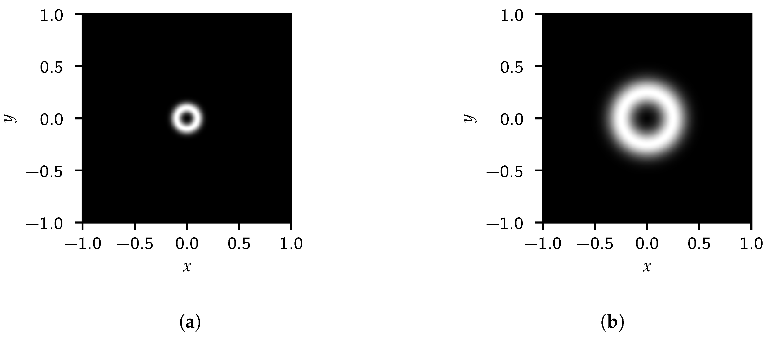
The first examples considered compare the effects of size on the FFT results. Only circular interfaces are considered. To generate a circular interface centered around
with radius
,
.
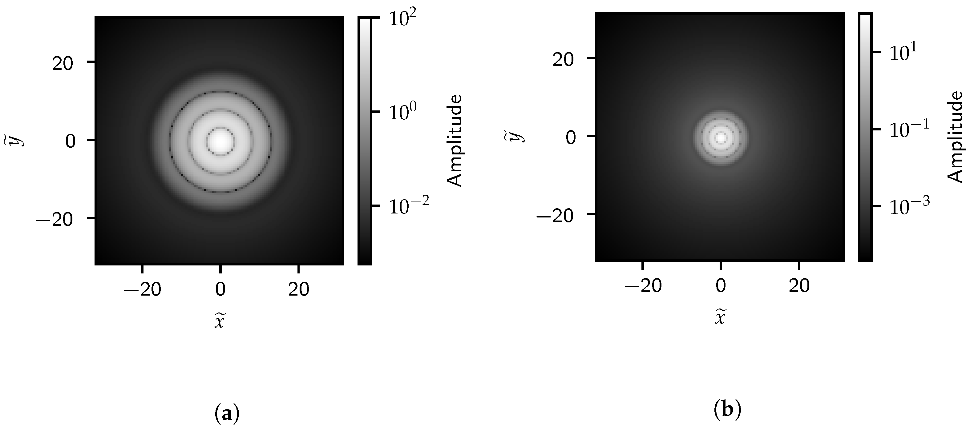
Figure 5 shows the images generated for circles with radius
and
centered at
, while
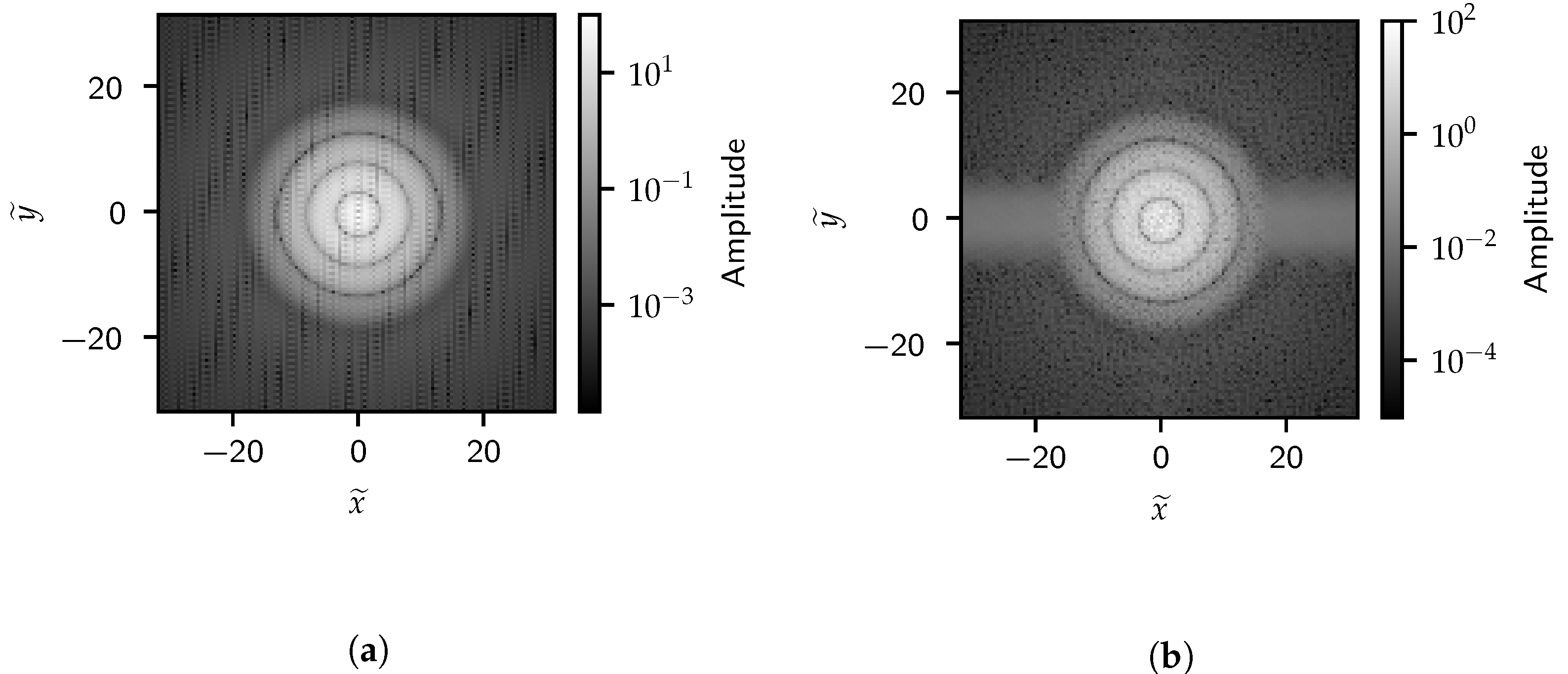
Figure 6 shows the corresponding 2D FFT results. Of course, since the original image has spherical symmetry, the 2D FFT results also show spherical symmetry.
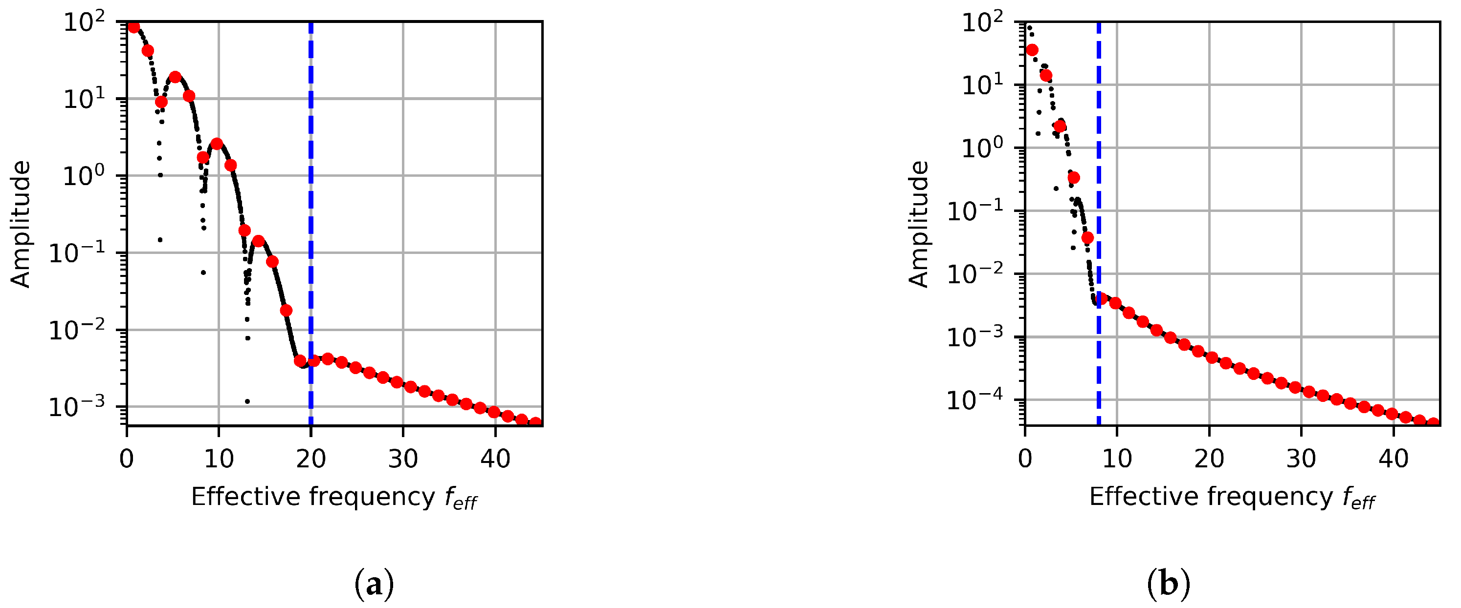
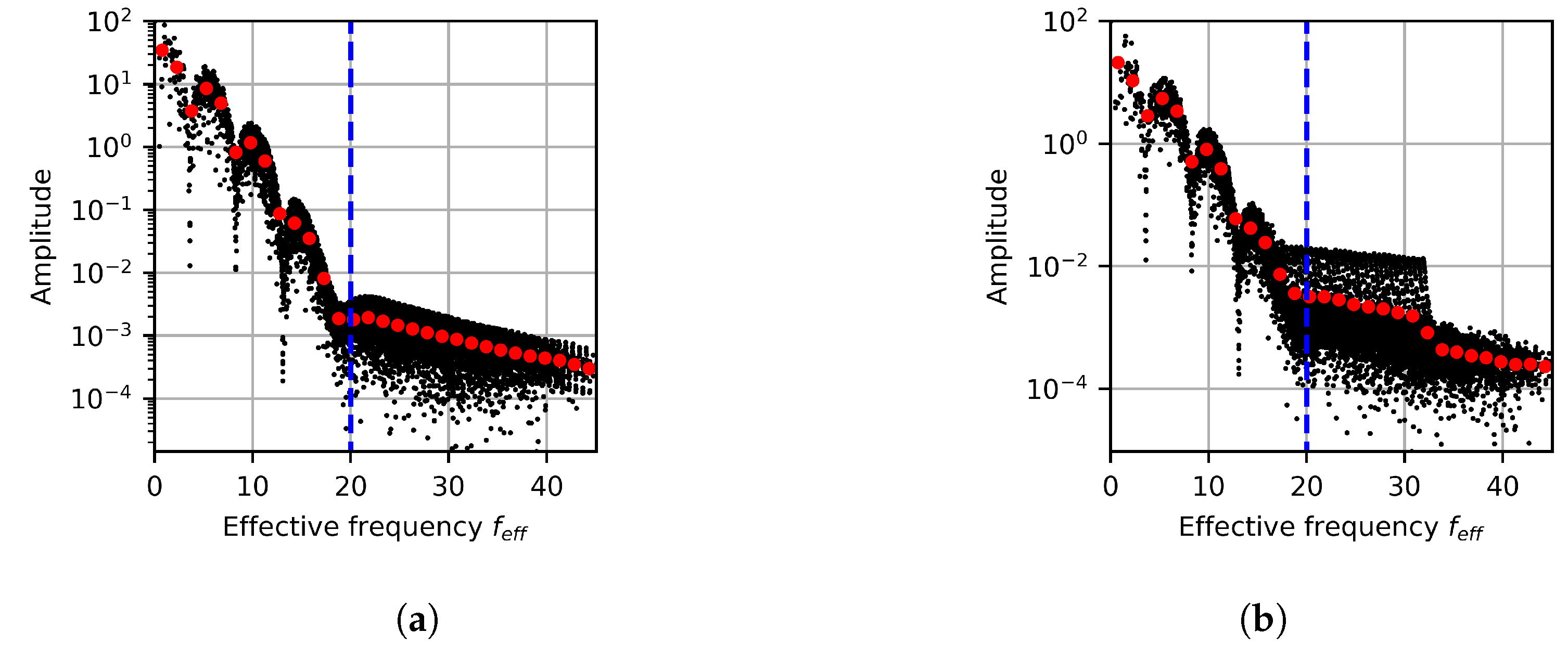
Figure 7 shows the 1D projection of the FFT results onto the effective frequency space. The blue dashed line in
Figure 7 indicates the effective frequency corresponding to
. For the remainder of this section, we refer to this frequency as the high-frequency length scale (HFLS) of
. Both the 1D and 2D FFT results highlight frequencies correlated to the circle radius and show that the image information is primarily contained in signals with frequencies lower than the HFLS. The amplitude of signals with frequencies above the HFLS is lower due to combined positive and negative inference of the complex exponential in the bands with a transition between low- and high-intensity. Several peaks can be seen over the low-frequency space. These peaks correlate to harmonics of the effective frequency corresponding to the diameter of the circle
.
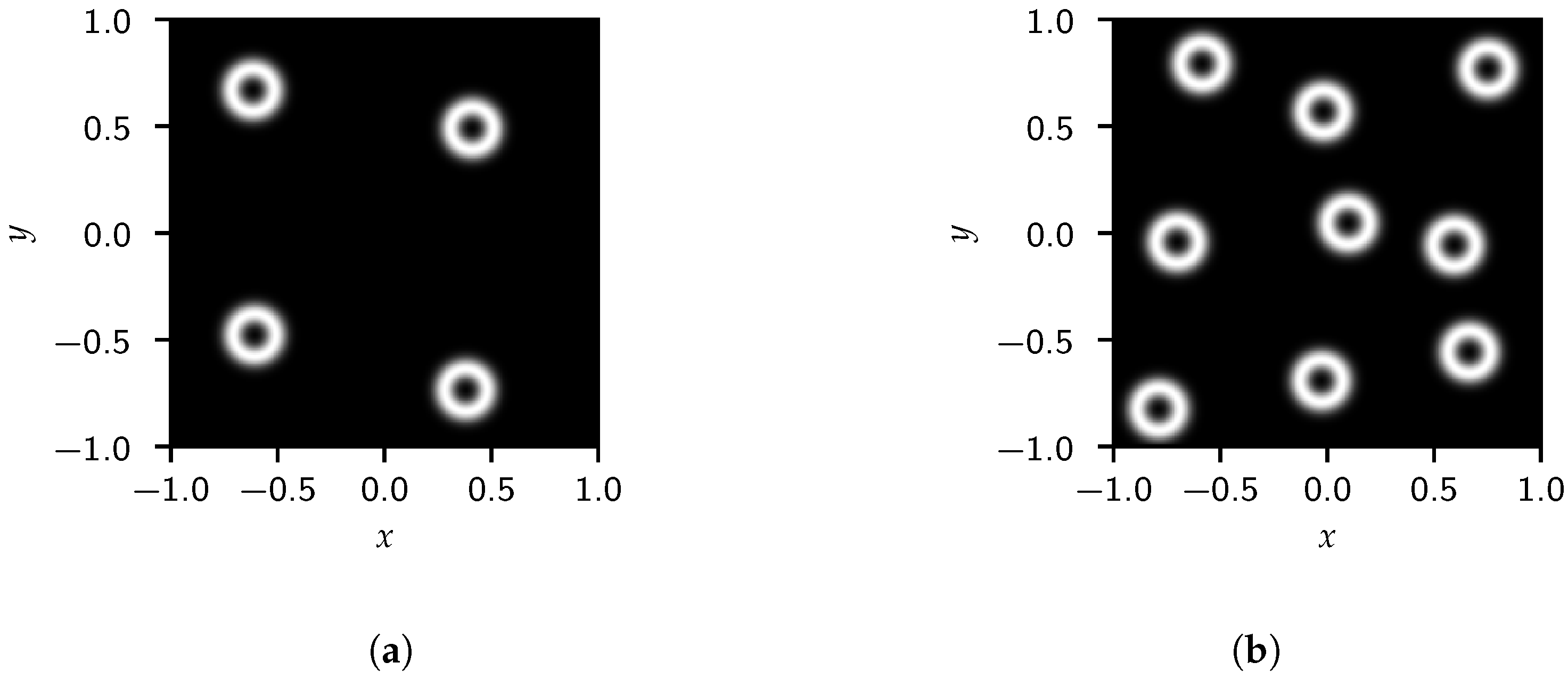
Next, the post-processing scheme is applied to cases with multiple objects that are randomly placed. All radii are set to 0.1 for this investigation. Again, two cases are compared, with the first having four objects and the second having nine. The generated images and their FFTs can be seen in
Figure 8 and
Figure 9, respectively, while
Figure 10 shows the 1D projections of the FFT data. The 2D FFT captures similar information as the single circle case, which unsurprisingly indicates the resilience of the FFTs against image transformation that preserves spatial structure. Besides information regarding individual circles, additional information is captured by the FFTs relating to how these objects are distributed in the domain as well. Of course, this is undesirable as it reflects information that does not correlate to the object size.
As with the single circle cases, the amplitude above the HFLS becomes more constant. This again makes this transition region indicative of the radius of the objects. Harmonics of the effective frequency associated with the diameter are again observed, albeit noisier. Although the FFT magnitudes associated with individual circles are similar, randomly placing circles shifts the phase of these signals. This pollutes the FFT amplitude of the full image over the effective frequency space making the raw FFT data less useful for identifying frequencies correlated with the object length scales. Fortunately, the averaged data still highlight the harmonics and HFLS.
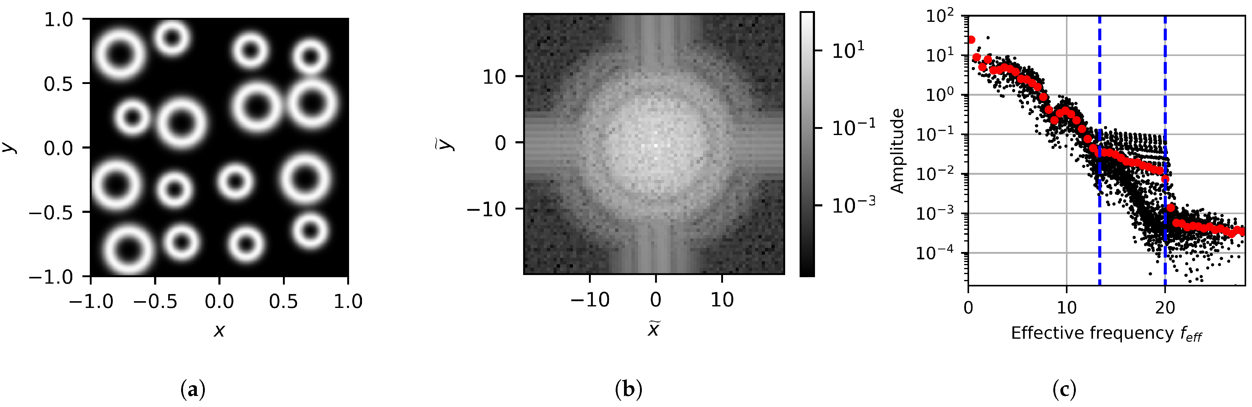
The scheme’s output when applied to an image of multiple objects of different sizes is also investigated. To generate this image, 16 circles are randomly placed, with each randomly sampling the binary set
to obtain its radius. The image and its FFT can be seen in
Figure 11a,b, respectively. The FFT results in the effective frequency space can be seen in
Figure 11c. Here, a dashed blue line is again used to indicate the HFLS; however, now two lines are drawn that correspond to both radii. As with the mono-sized case, the regions where transitions between slopes occur correlate to the sizes of the circles in the image. Objects of similar size primarily contain low-frequency terms up to their HFLS. Adding larger features increases the information over a lower-frequency subset of the smaller objects’ primary frequency space. As such, a change in slope is indicative of different feature sizes. However, the distinction between different sizes is less obvious, especially when compared to the transition at the largest HFLS. This is due to the exponential decay of amplitude over frequency as well as the FFT containing additional information about the positions of objects relative to each other. However, the averaged amplitude again assists in making the distinction clearer.
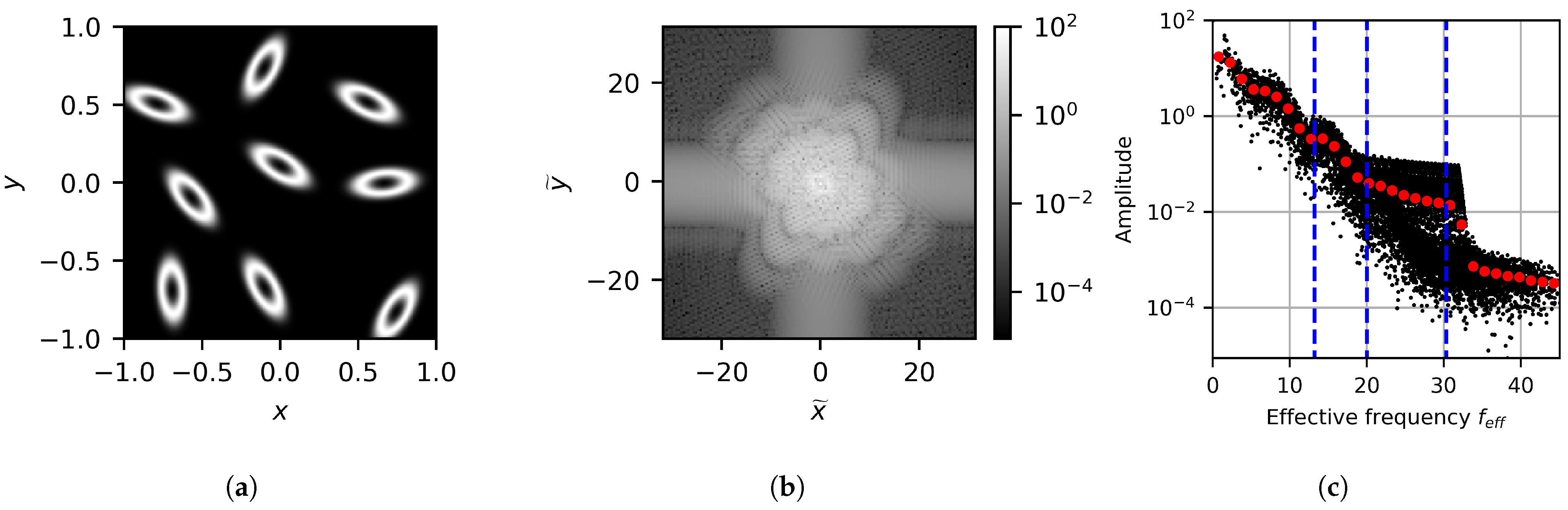
Finally, the last set of results considers the effects of deforming the interfaces. To achieve this, the circles are stretched into ellipses along random directions. The area of these ellipses is kept constant and is equivalent to that of a circle with a radius of 0.1, and the eccentricity of the ellipse is set to 0.9. In this case, the image is generated with nine ellipses, as shown in
Figure 12a. The FFT results can be seen in
Figure 12b,c, where the 2D and 1D projected results are provided, respectively. When compared to the case with nine circles, similar structures in the radial direction can be seen in the 2D results. However, instead of spherical symmetry in the frequency space, strong directionality linked to the orientation of the ellipses in physical space is observed. Of course, since the FFT is a linear operation, the more interfaces with disordered directionality there are, the more uniform this would become. For the 1D results, rather than only indicating the radius, now the dashed blue lines are used to indicate the HFLS associated with the major axis, the equivalent radius, and the minor axis of the ellipse. As expected, the FFT results correlate to both spatial length scales associated with the interface shape as well as the equivalent length scale related to the volume. However, this also highlights that naively applying this approach can result in the extraction of length scales that correspond to different features of the same object.
3.2. Quantification of Nozzle Atomization for Comparison
The main result of this work considers the application of the post-processing scheme to the outlet condition of a liquid–gas atomizer nozzle. With the degree of atomization being a core performance metric for atomizer nozzles, comparing nozzle designs is ideal for demonstrating the ability of the proposed FFT post-processing scheme to quantify the length scales of atomization. The post-processing scheme’s construction is directly applied without any explicit knowledge about the profile geometry or the outlet conditions while keeping the results comparable due to similar length scales between simulations. The nozzles chosen for this study are based on typical atomizer nozzle designs. Considerations were made to ensure the designs are similar in terms of bulk flow behavior while still encouraging the development of unique outlet flow patterns.
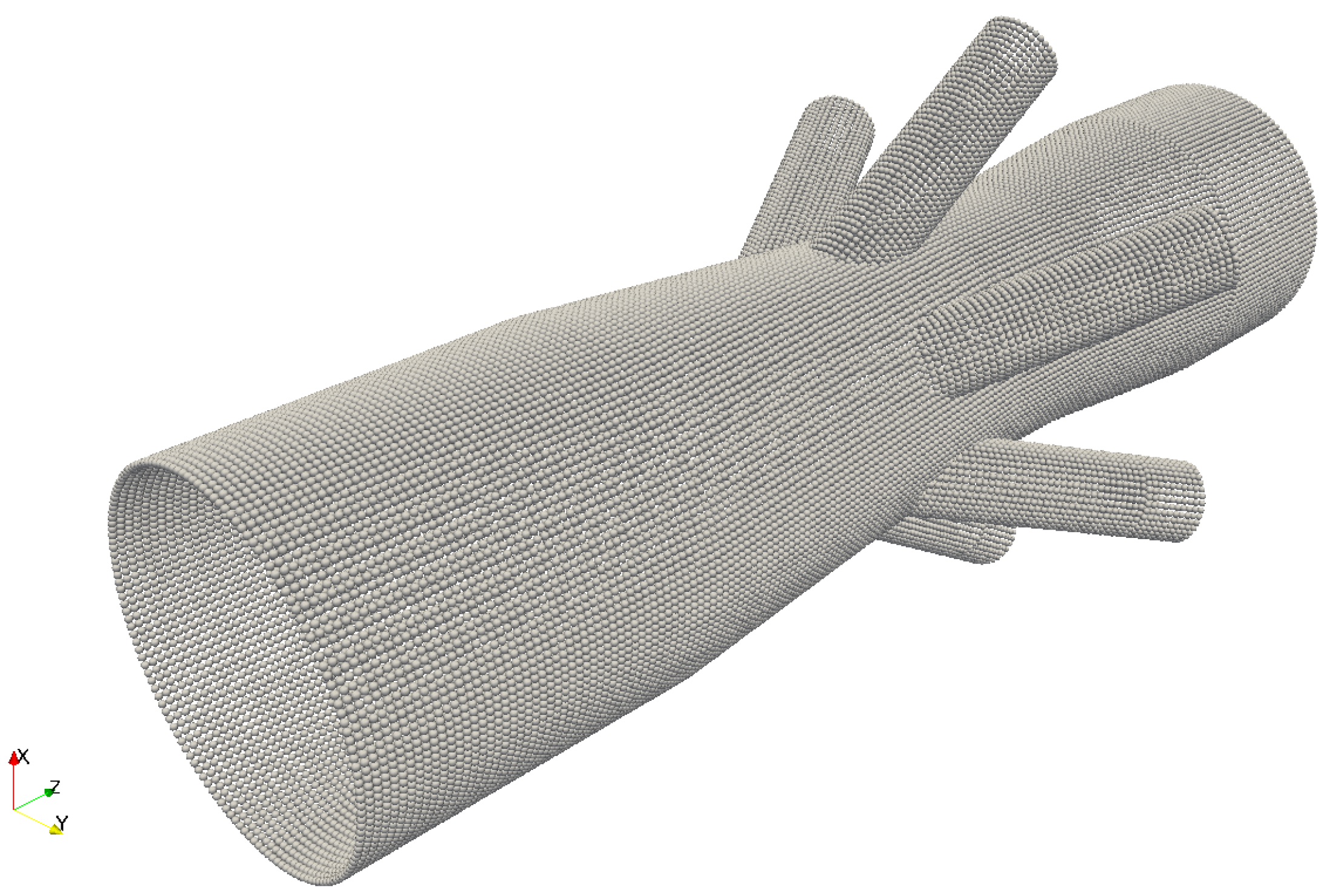
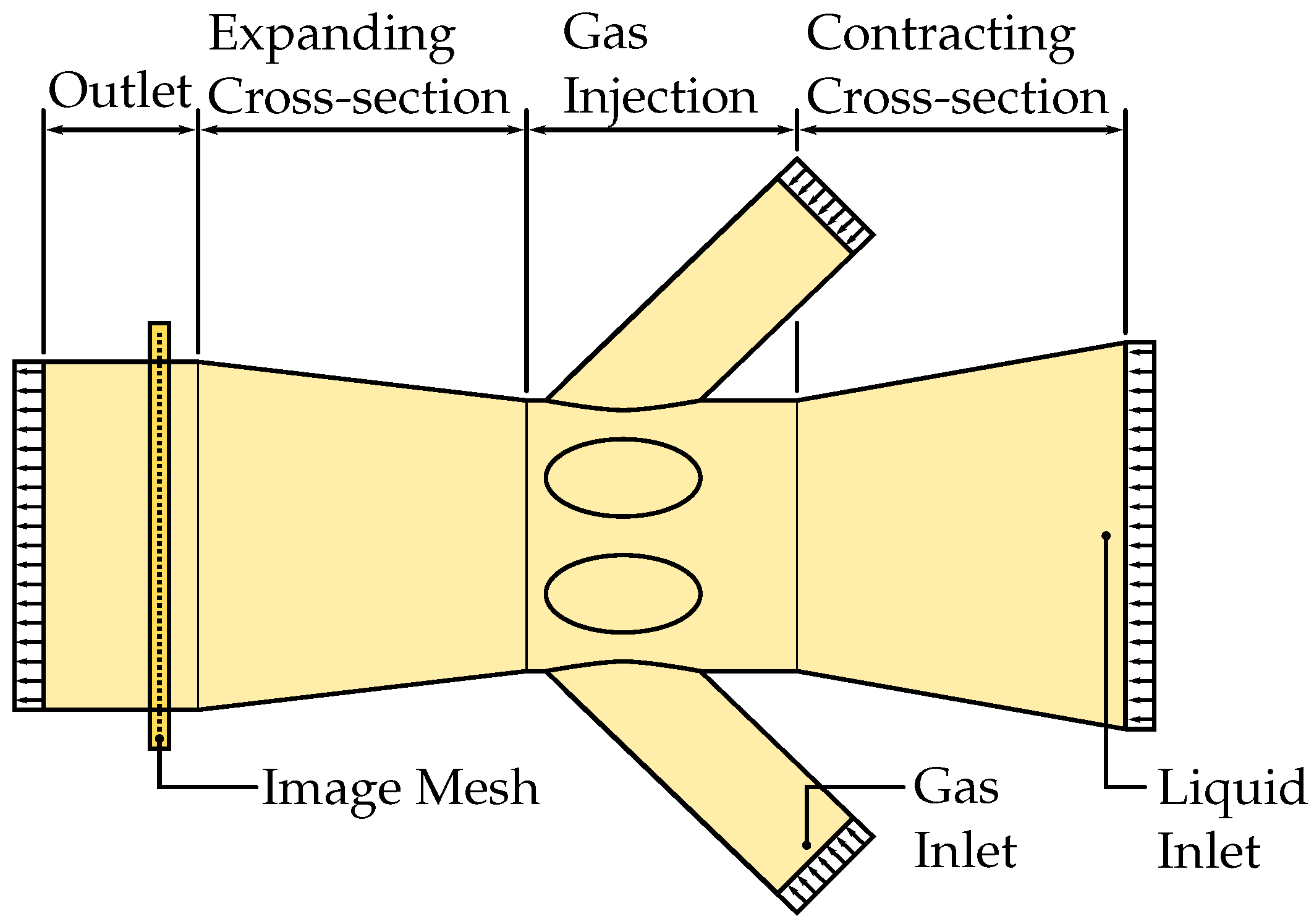
Two nozzle designs are investigated in this work. An example of one of the nozzles can be seen in
Figure 13, while
Figure 14 shows a schematic description of the nozzle. The nozzle topology is identical for both cases. The main pipe carries a high-density, high-viscosity fluid into the system. This pipe gradually contracts and, at its minimum diameter, has high-pressure gas injection into the system. This two-phase mixture is then subject to pipe expansion. The difference between the cases comes from the profiles of the pipes. Specifically, this study carries out a comparison between nozzles with cylindrical and elliptical outlets. The area of the profiles is kept constant, leading to both cases having the same mass flow rate. The density ratio between the fuel and gas is 220:1. The system was simulated for 2.5 ms with the 200 images uniformly sampled between 0.5 ms and 2.5 ms. The fluid system was discretized by 134 k particles.
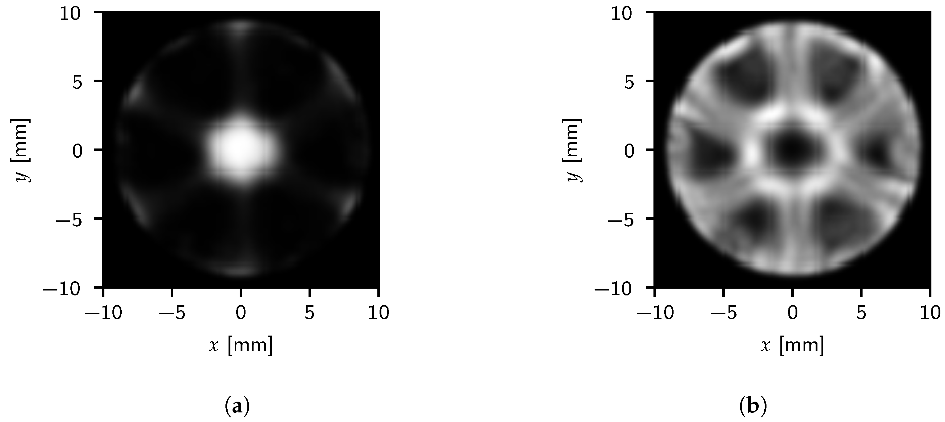
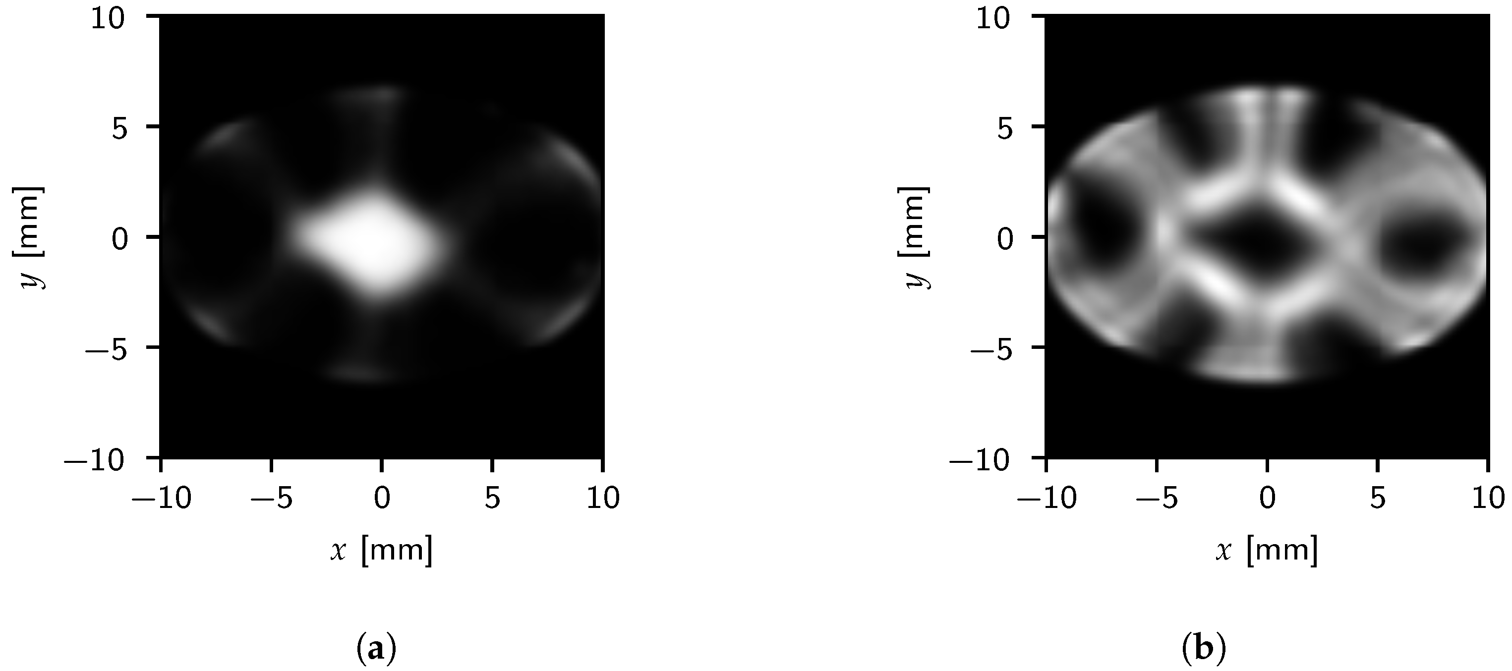
Figure 15 and
Figure 16 show the images generated with both the outlet density and color gradient magnitude data for the cylindrical and elliptical cases, respectively. The color gradient does indeed capture the interface between fluids. Furthermore, the benefits of using the color gradient can be seen as it highlights fine structures due to diffuse mixing as well.
For the color gradient images, a higher intensity corresponds to a sharper interface, while zero corresponds to a single-phase region. Both the cylindrical and elliptical cases show a central fuel column surrounded by six gas columns. Between gas columns, a region of moderate intensity indicates a mixture between fuel and gas. Besides the obvious outlet shape effects, from a qualitative standpoint, both geometries generate similar responses.
3.2.1. Two-Dimensional Spectral Analysis
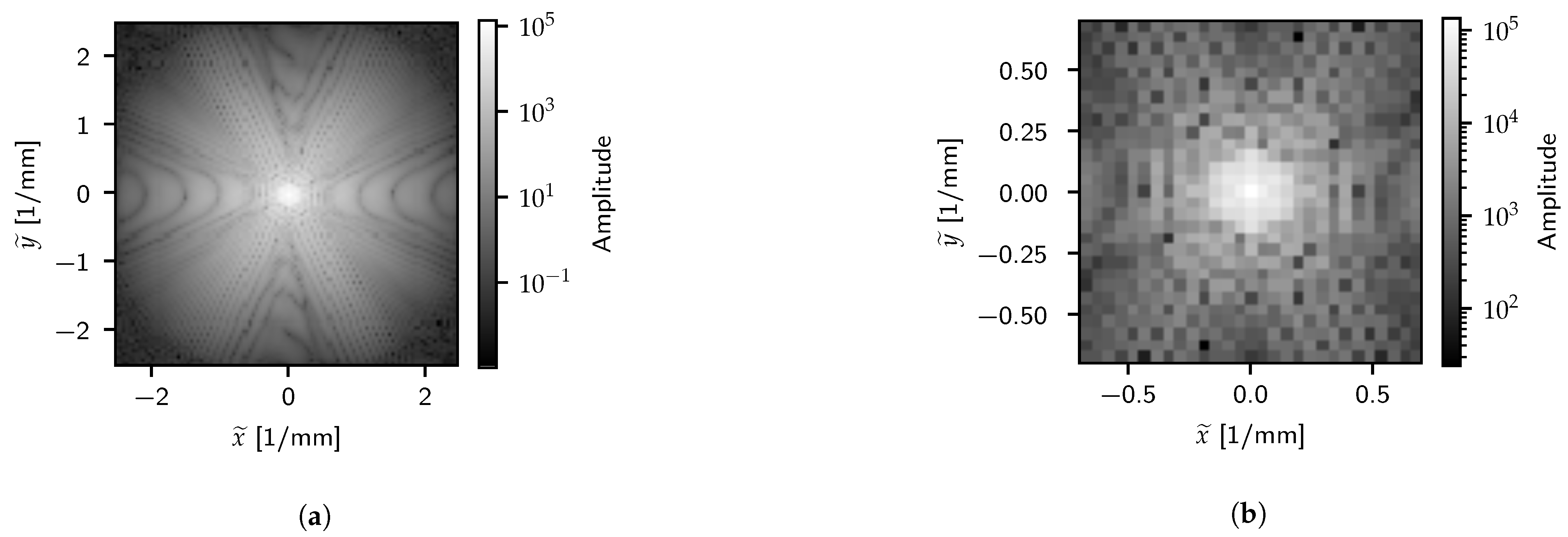
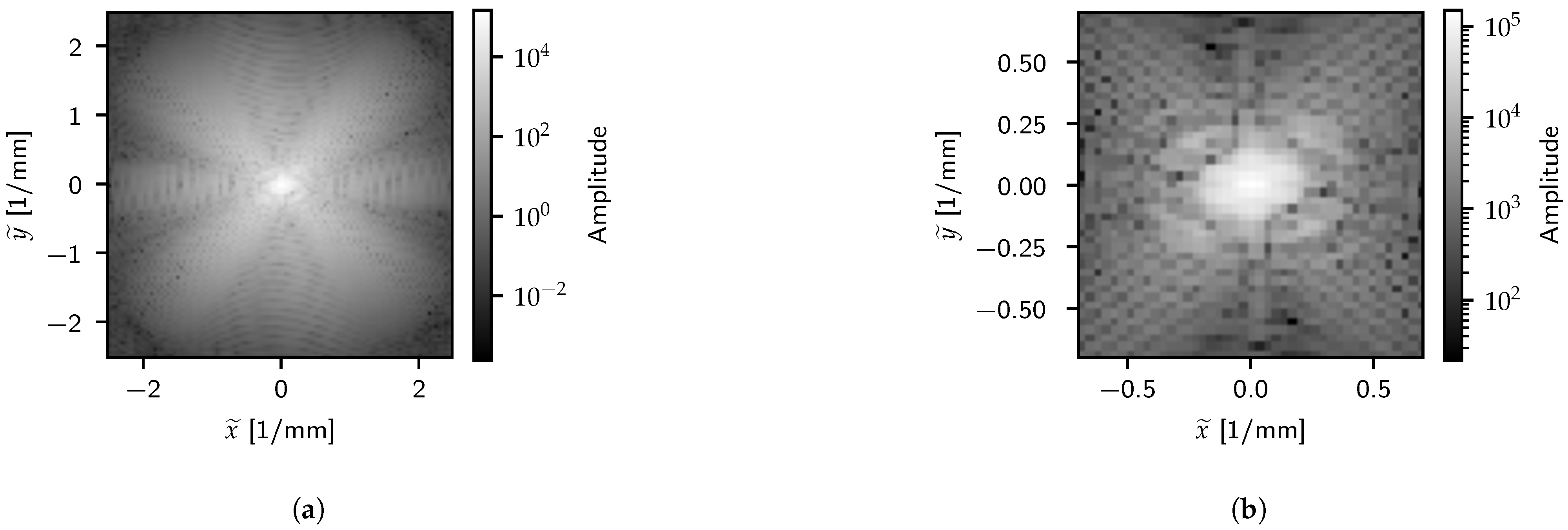
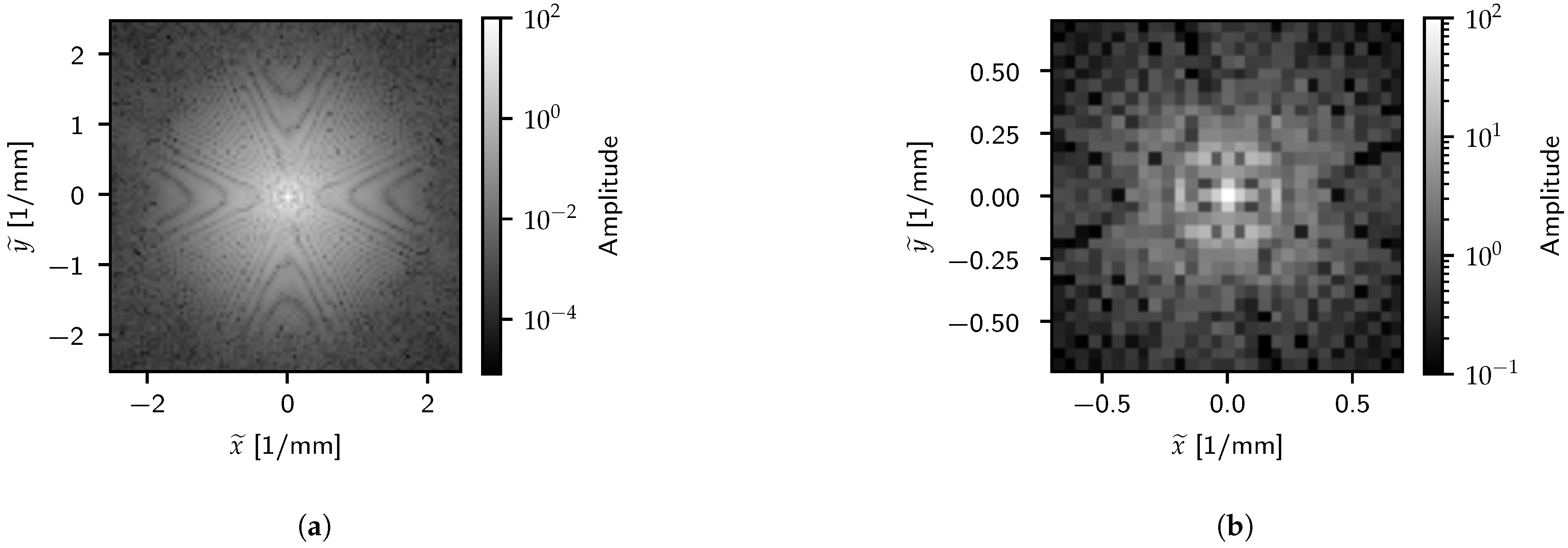
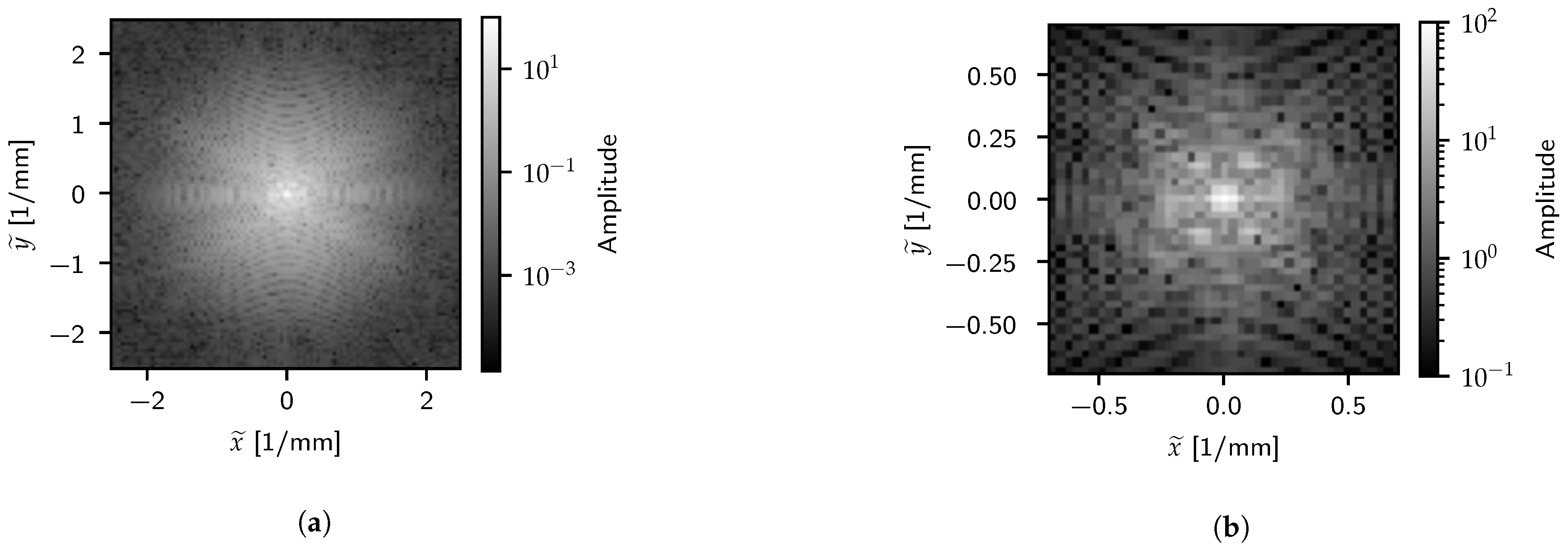
The corresponding spectral results for density can be seen in
Figure 17 and
Figure 18, while the color gradient results can be seen in
Figure 19 and
Figure 20. As with the spatial results, the effects of the outlet geometry can be seen in the frequency space results as well, especially when considering the low-frequency region. However, these results already highlight subtler differences between the cases as well. By looking at the low-frequency domain and even the full-frequency color gradient results, the cylindrical geometry has more dominant low-frequency terms, while the information in the elliptical case is distributed further into higher-frequency regions.
When comparing the density and color gradient results, both highlight similar large-scale structural patterns in the image. However, the high-frequency density results are more strongly dominated by the macroscopic structures due to the density fields lacking high-frequency information. Since the color gradient image more clearly resolves mixing information compared to the density, the FFT highlights these features in frequency space as well. This is especially clear in the low-frequency domain, where the color gradient results show refined details compared to the coarser structures obtained with density. While the density image demonstrates this scheme’s behavior on fluid volumes, the low-fidelity nature of these simulations makes it less suitable for this investigation. As such, the remaining results only operate on the color gradient results.
3.2.2. 1D Spectral Analysis
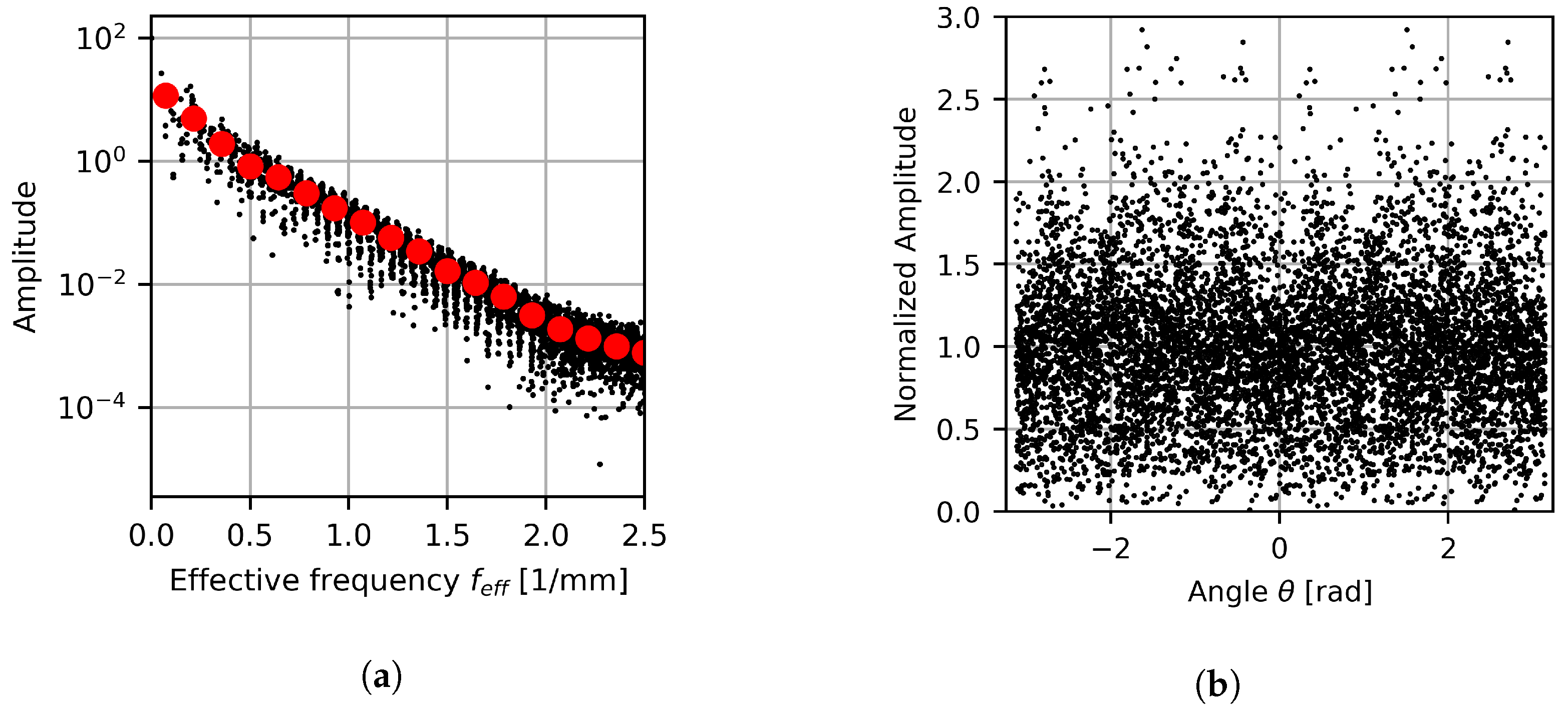
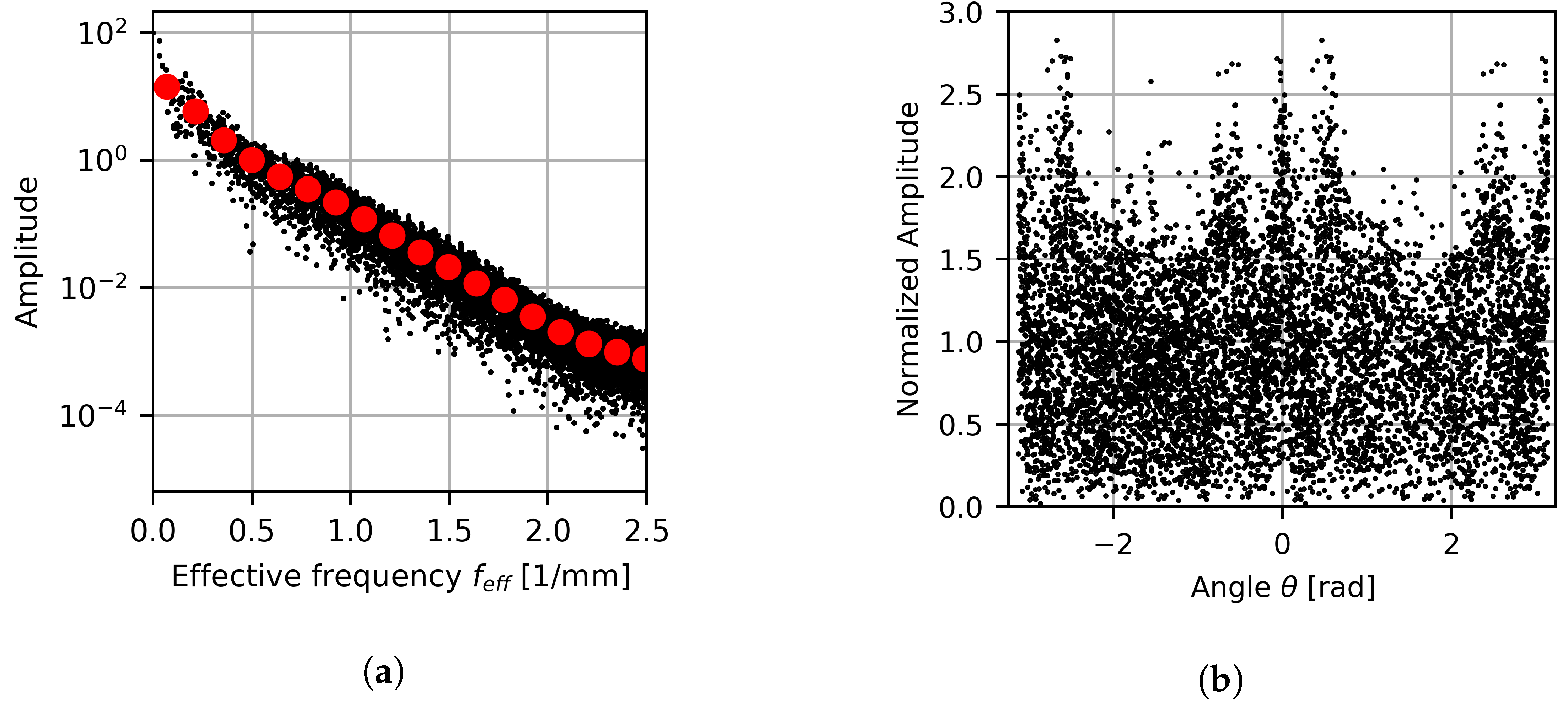
Figure 21 and
Figure 22 show the projection of the 2D spectral data onto the 1D effective frequency space and angle projection for the cylindrical and elliptical case, respectively. The binned results are also shown for the effective frequency results, with 18 bins being used for each result set. When considering the angular projection results, peaks occur at regular intervals for the cylindrical case, while the elliptical case’s peaks are irregularly spaced. These highlighted regions coincide with the angles in the spatial domain where gas columns form. The elliptical case’s peaks are more pronounced, indicating a tendency for flow features to form in the directions of the gas columns more readily. This is expected since the cylindrical case’s gas columns are more isotropic, leading to unaligned flow features being more likely. Even so, the order of magnitude of dominant features is similar over all angles. This implies that although there are preferred directions, structure in the color gradient magnitude is still well distributed with no directions completely dominating the response for either case.
When considering the effective frequency projection, exponential decay is seen over the frequency space. Furthermore, the results can be divided into three regions characterized by their frequency: a low-frequency range from 0 to 0.5 , a mid-frequency range from 0.5 to 2.0 , and a high-frequency range of 2.0 to 2.5 . These regions have different decay rates, with the decay rates decreasing with an increase in frequency.
The reason for these regions forming is due to the intrinsic length scales present in the system. The low-frequency region is of the order of the large-scale gas and liquid column structures, while the high-frequency region captures behavior at the GFD particle length scale. The mid-frequencies represent the remaining system information, which relates to information at the fluid interface level. As such, low-frequency results provide information about the large fluid volumes, while mid-range frequencies describe the diffuse mixing between phases. The reason for the high-frequency results plateauing is due to the lower likelihood of structured arrangements forming from individual particles.
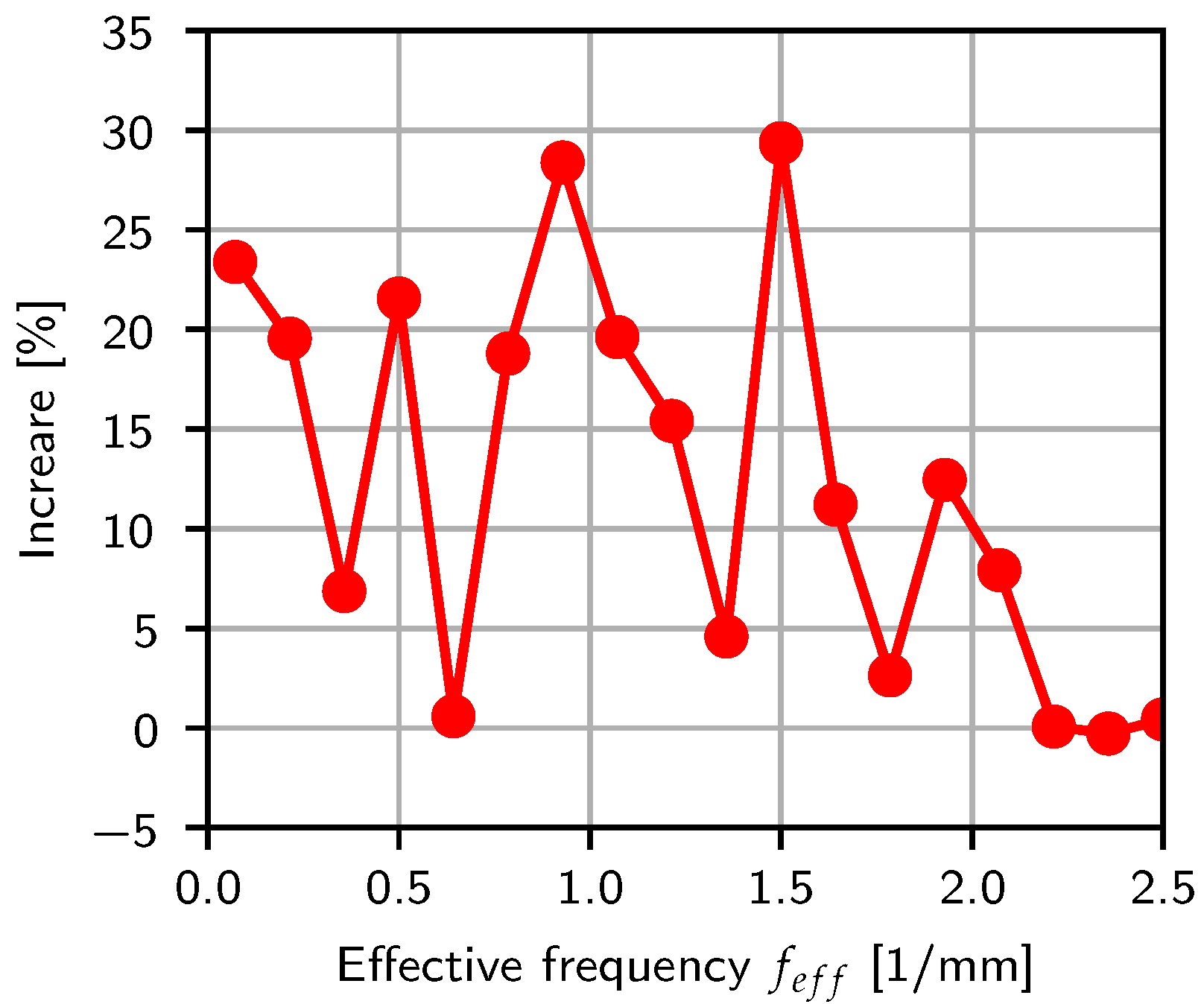
Using the cylindrical profiles as the baseline, a comparison of the binned results is performed.
Figure 23 shows the percentage increase in the elliptical case relative to the cylindrical case. This highlights the significance of the nozzle geometry, with the ellipse showing a significant improvement over most of the spectrum with only similar behavior being observed close to the particle scale. Over the full spectrum, an increase of 12.36% is obtained on average.
4. Conclusions
A post-processing scheme was proposed for the quantitative comparison of multiphase interfaces generated during the primary atomization of a viscous liquid–gas system. By considering the multiphase interface from a spatial frequency perspective, the fluid behavior over the system length scales could be quantified and compared.
A verification study was performed that highlights the behavior of the proposed scheme in a controlled setting. The results show that by applying a 2D FFT on an image of finite-width interfaces, it is possible to identify information regarding both the shape and volume information of the underlying objects. However, as a result of abstractly analyzing the image data, the interpretability of the output is lowered. Although information of interest is present in the spectral data, length scales in the spatial domain must first be identified before they can clearly be related to information in the frequency space. As such, if applied to simulation results with the desire to extract information such as the SMD, it will be required to couple this with an experimental study that captures both the frequency spectrum and the SMD distribution to construct a correlation between the data sets.
However, for quantification, this technique can be applied directly in its more abstract form. When applied to atomizer nozzles, distinct features were identified in the spectral response that provided quantitative evidence for preferring certain nozzle designs. Furthermore, this was achieved by following an algorithmic approach making this appropriate not only for design but also for optimization of devices operating in multiphase environments. With the simulation results being low fidelity, the scheme has only been shown in the context of primary atomization. However, it is expected that this scheme would be appropriate for finer resolved fluid structures, as shown in the verification study. However, with industrial-scale simulation usually making use of Lagrangian droplet generation methods directly, many numerical schemes may prefer to directly use this information for quantification.
While the post-processing scheme does decompose information according to length scale, it is important to note that this does not relate to physical droplet sizes. Furthermore, it should be mentioned that the comparison between nozzle designs used in this work is based naively on the total frequency spectrum. However, it may be possible to identify subsets numerically or experimentally as having a more dominant effect on the performance metrics of interest. As such, it is recommended that the collection and processing of atomization data in the context of the proposed scheme be further investigated as a way to relate the spectral results to more typical performance metrics.


