Article

A Generalized Finite Difference Scheme for Multiphase Flow

by
Johannes C. Joubert
1,*,
Daniel N. Wilke
1 and
Patrick Pizette
2
1
Department of Mechanical and Aeronautical Engineering, University of Pretoria, Private Bag X20, Hatfield 0028, South Africa
2
IMT Lille Douai, Univ. Lille, EA 4515-LGCgE Laboratoire de Génie Civil et géoEnvironnement, CERI Matériaux et Procédés, F-59000 Lille, France
*
Author to whom correspondence should be addressed.
Math. Comput. Appl. 2023, 28(2), 51; https://doi.org/10.3390/mca28020051
Submission received: 14 February 2023 / Revised: 20 March 2023 / Accepted: 23 March 2023 / Published: 26 March 2023
(This article belongs to the Special Issue Current Problems and Advances in Computational and Applied Mechanics)

Abstract

:
This paper presents a GPU-based, incompressible, multiphase generalized finite difference solver for simulating multiphase flow. The method includes a dampening scheme that allows for large density ratio cases to be simulated. Two verification studies are performed by simulating the relaxation of a square droplet surrounded by a light fluid and a bubble rising in a denser fluid. The scheme is also used to simulate the collision of binary droplets at moderate Reynolds numbers (250–550). The effects of the surface tension and density ratio are explored in this work by considering cases with Weber numbers of 8 and 180 and density ratios of 2:1 and 1000:1. The robustness of the multiphase scheme is highlighted when resolving thin fluid structures arising in both high and low density ratio cases at We = 180.

1. Introduction

Multiphase fluid flow is a physical phenomenon involving the interactions arising between several immiscible fluids, often with strong coupling between phases. Aside from being a fundamental feature in various natural systems, multiphase flow is often introduced and exploited in engineering contexts, with multiphase flow enabling the core operational mechanisms of solutions in various industries including oil and gas production, power generation, and chemical processing. As such, it is crucial to understand these systems from both the design and analysis perspectives. However, the complex dynamics arising from the interaction between immiscible fluids are often difficult to resolve. The primary challenge with multiphase flows comes from the need to resolve a Lagrangian interface between fluids. With Eulerian methods being a common choice for computational fluid dynamics (CFD) solutions in general, early strategies involved simulating multiphase systems with a range of meshed methods to resolve the multiphase interface. These include volume of fluid (VOF) methods [1,2] or finite-volume methods (FVMs) with a front tracking (FT) [3] scheme. However, the recent interest in meshless Lagrangian methods (MLMs) has resulted in a surge in meshless schemes relying on their natural resolution of Lagrangian information to trivially handle interface tracking.
With particle-like nodes that are free to flow according to the velocity field, MLMs discretize the initial domain with the particles of a specific fluid type and resolve the interface kinematics via node updates directly. Although interfaces are naturally resolved, additional work must be carried out to introduce surface tension effects. A common strategy employed in MLM schemes adopts the continuous surface force (CSF) model first introduced by Brackbill et al. [1] to resolve the surface tension force in a multiphase FVM context. In an MLM context, this model operates by assigning each particle a color value. Meshless differential operators act on the color field to resolve the interface normal and surface curvature, which in turn are used to determine the surface tension force. Various color functions have been proposed. Several studies [4,5] opted to treat color as a discrete binary state that is used to indicate different phases when resolving the interface normals. These models have been extended to incorporate material properties by basing the color’s intensity on the material density [6,7,8,9]. Alternative approaches smooth out the transition between phases, allowing for mixing and diffusion between phases to be handled from a continuum perspective [10,11,12,13].
For similar fluid properties in orderly flow conditions, it is possible to model the fluids discretely at the particle level. However, this strategy may lead to instabilities as mixing becomes more prevalent or material properties become more dissimilar. As such, it is typical for MLMs to utilize a material mixing model for particles in the interface support region [10,13,14].
As one of the most common MLMs, smoothed particle hydrodynamics (SPH) has been extensively used to simulate multiphase flow. However, a drawback of classical SPH models modified for multiphase environments arises from its use of the weakly compressible (WC) model for mass–momentum coupling. Although several multiphase WCSPH schemes have been proposed, the coupling between pressure, density, and the artificial speed of sound poses significant challenges when dealing with large density ratios. A common strategy is to relax the incompressibility constraint on the lighter phase by controlling the equation of state’s polytropic constant and speed of sound per phase [8,15,16,17,18]. This, however, has a detrimental effect on the time step size at large density ratios [16]. The use of a global artificial speed of sound for all phases has also been explored [19,20,21]. Although this lowers the speed of sound for the light phase, it also limits the maximum pressure that the light phase can resolve while still satisfying the incompressibility condition. Again, this relaxation becomes more significant for larger density ratios. Despite this behavior, modern multiphase simulations such as the work of Vahabi and Kamkari [22] show that these strategies make WCSPH a viable choice for high density ratio simulations, even when treating non-Newtonian fluids. The work of He et al. [23] proposed a solution to treat high density ratios by modifying the SPH pressure gradient. By only considering similar phases when constructing the density approximations, a more robust estimate can be generated. This in turn improves the pressure obtained from the WC equation of state.
An alternative strategy is to abandon WC models completely and use a truly incompressible scheme [24]. Aside from removing the need for an artificial speed of sound, this also avoids the need for corrective terms to smooth the typically noisy pressure field present even in single-phase simulations [25,26]. Despite this, high density ratios can still pose problems for incompressible solvers, as spurious fragmentation may still be observed in highly dynamic flow environments [11,21,27,28]. A solution to this was proposed by Xu et al. [29], where the fully Lagrangian approach was extended by coupling an incompressible SPH solver for the light phase with an FVM for the heavier phase. This approach exploits the benefits provided by the Lagrangian perspective of SPH to resolve fluid interfaces effectively. While this approach was shown to treat high density ratio cases robustly, the scheme’s complexity is significantly increased when compared with purely Lagrangian approaches.
Although SPH has been extensively applied to multiphase modeling, these schemes are modified to address typical issues, such as high-frequency noise in its pressure solution [21]. Furthermore, although more sophisticated color functions and mixing models have been explored within an SPH context, they are typically utilized for the improved stability they offer by smoothing the transition between phases. With the surface tension resolution dependent on the color gradient, its accuracy and robustness are strongly coupled to the quality of a scheme’s differential operators. For this reason, multiphase schemes often rely on the more computationally expensive first-order accurate differential operators to resolve surface information [5,9,30,31]. However, it has been shown that generalized finite difference (GFD) differential operators are more computationally efficient than similar first-order accurate SPH operators [32]. Furthermore, it has also been shown that the GFD method is suitable for incompressible flow simulation [33] and has already been applied to multiphase environments as well [34].
As such, this work proposes an incompressible, multiphase GFD scheme based on the scheme presented in [34]. This scheme is extended by introducing a dampening model to treat spurious oscillation formed on the surface of high density ratio interfaces. The interface and surface tension models are verified against analytical and numerical solutions. Finally, the scheme is used to simulate droplet coalescence and break-up. Although cast in the context of the incompressible GFD, the proposed methods are well-suited for MLMs in general.

2. Materials and Methods

2.1. Incompressible General Finite Difference Method

As with other MLMs, the GFD method discretizes the computational domain using a point cloud of an approximately uniform density. Each node, commonly referred to as a particle, is assigned pointwise information of the fields present in the partial differential equation (PDE). With no connectivity between points, the computational nodes are free to resolve advection operators by directly updating their positions. This requires the PDE to be considered in a Lagrangian frame. For this paper, the Navier–Stokes equations (NSEs) for incompressible multiphase flow are considered:
· u = 0 ,
d u d t = p ρ + 1 ρ · 2 μ T + g + s ,
with u being the velocity, p being the pressure, ρ being the density, μ being the dynamic viscosity, T = 1 2 ( u + u T ) being the symmetric strain rate tensor for incompressible flow, g being the acceleration due to body forces, and s being the acceleration due to surface tension, as discussed in Section 2.2.
It should be noted that the presented scheme resolves the viscous diffusion term as follows:
· 2 μ T = μ 2 u + μ · 2 T .
To resolve the differential operators, the finite differences between neighboring particles are weighted by a kernel function. These kernels usually have a finite support radius. This limits the number of interactions that must be resolved and thus drastically improves the computational cost scaling. This work makes use of the quintic kernel [35]:
W ( r , h ) = ( 3 q ) 5 6 ( 2 q ) 5 + 15 ( 1 q ) 5 for 0 q 1 ( 3 q ) 5 6 ( 2 q ) 5 for 1 < q 2 ( 3 q ) 5 for 2 < q 3 0 otherwise with q = r / h ,
with r being a position vector, 3 h being the support radius of the kernel, and · indicating the Euclidean norm. It should be mentioned that, as with other renormalized or gradient-corrected schemes, the kernel function does not need to be normalized for the GFD method.
When applied to a pair of nodes i and j located at r i and r j , respectively, the kernel function operating on the relative position r i j = r i r j can be thought of as a measure of the diffusion of node j’s information to node i. For readability, the notation W i j = W ( r i j , h ) is adopted in this work. Furthermore, for a general field f, the field value at the i t h particle f ( r i ) is represented by f i .
The kernel function also serves to identify neighboring points by allowing the indexing set of all particles neighboring the i t h particle to be defined as I = j Z / N Z : W i j > 0 , where N is the number of nodes in the system.
The gradients of Lanson and Vila [36,37] and the Laplacian of Basic et al. [38] are used in this work. For a general field f, the differential operators are resolved as follows:
f i = B i · j I f i f j W i j r i j ,
2 f i = 2 d j I f j f i W i j 1 r i j · o i j I r i j 2 W i j 1 r i j · o i ,
with d being the system dimension and
B i = j I W i j r i j r i j 1 ,
o i = B i · j I W i j r i j .
representing the truncation tensor and offset vector, respectively.

2.2. Multiphase Model

Multiphase physics introduces an additional surface tension forcing condition at fluid interfaces. As the model used in this work is based on the CSF formulation [1], the scheme strongly relies on the so-called color function. This function typically operates by assigning each particle an integer value identifying the phase. To resolve the surface interfaces and their associated normals, the GFD gradient is applied to the color field.
Due to the violent mixing taking place between phases, assigning an integer color value would generate a noisy color gradient. Rather, a mixing model is used to describe the amount of each color present at each node. The color of the i t h node for the n t h phase is given as follows:
C i n = j I n W i j j I W i j
with I n being the set of all nodes in the support radius of I and in the n t h phase.
The color gradient is used to resolve the interface normals. Since this work only considers two fluids, the gradient is only determined for the first color C 0 . The normal direction n i is then determined as follows:
n i = C 0 ρ i = B i · j I C i 0 C j 0 ρ ¯ i j W i j r i j
with ρ ¯ i j = 1 2 ( ρ i + ρ j ) being the average density.
Following the scheme proposed in [17], interface particles are identified by filtering the color gradient magnitude. As such, each particle is assigned a normal according to
n ^ i = n i n i if ρ i n i > ϵ h 0 otherwise
with ϵ being a user-specified parameter to control the aggressiveness of the filter. As suggested in [17], ϵ = 0.01 was found to be appropriate for all simulations in this work.
The curvature κ is resolved from a filtered color gradient approximation:
κ i = · n ^ i = j I I m W i j n ^ j n ^ i · B i · r i j
with I m = j Z / N Z : ρ i n i > ϵ h being the indexing set of all particles bypassing the filter. This check ensures that the interface support region remains localized around the interface and thus limits the effects of parasitic currents intrinsic to the CSF model.
The acceleration due to surface tension is then resolved as follows:
s i = σ · n ^ i C 0 ρ i ,
with σ being the surface tension coefficient.
Due to the smooth spatial evolution of Equation (9), the color field also allows local fluid properties such as the viscosity and density to be resolved as weighted averages:
ρ i = n ρ n C i n
ν i = n ν n C i n
with ρ n and ν n being the density and viscosity of the n t h phase, respectively.
The momentum diffusion operator of [34] is used in this work. As such, the viscosity gradient is determined as follows:
μ ρ i = ( μ 0 μ 1 ) C 0 ρ i ,
with μ 0 and μ 1 indicating the dynamic viscosity of the first and second phases, respectively.

2.3. Time Integration Scheme

To integrate the semi-discretized system, a projection-based scheme like incompressible SPH (ISPH) [26] is followed. Specifically, each time step is split into an update and projection step. The update step considers the viscous momentum diffusion, body force, and surface tension updates. For the k t h update step, we have
u i * = u i k + Δ t ν i 2 u k i + μ ρ k i · 2 T k i + g i + s i k ,
with u i * being an intermediate velocity and Δ t being the time step size. It should be noted that Section 2.5 modifies this equation by including a dampening term.
The pressure Poisson equation (PPE) is used to resolve node pressures based on the divergence of the intermediate velocity field:
2 p k + 1 ρ i = 1 Δ t · u * i .
The density field may become noisy when violent mixing takes place. To introduce smoothing, the average density is used to scale each finite-difference term. As such, the Laplacian of Equation (6) is modified as follows:
2 p ρ i = 2 d j I p j p i ρ ¯ i j W i j 1 r i j · o i j I r i j 2 W i j 1 r i j · o i ,
It should be noted that this Laplacian reduces to 2 p i / ρ i for any fluid particle whose support radius does not intersect the support domain of the multiphase interface.
Considering that the differential operators are linear with respect to their primitive variables, Equation (18) may be represented as a sparse large linear system. Section 2.4 discusses the construction and solution scheme of this equation in more detail.
To enforce the divergence-free condition, we have
u i k + 1 = u i * Δ t p k + 1 ρ i ,
with
p ρ i = B i · j I p i p j ρ ¯ i j W i j r i j .
Rather than resolving the pressure gradient directly, this form is chosen, as it inherently smooths the density field at fluid interfaces and thus improves upon the numerical stability of the scheme. It should be noted that since the density is only modified at a fluid interface, this form also reduces to p i / ρ i for any particle whose support radius does not intersect with the multiphase interface’s support domain.

2.4. Pressure Poisson Equation

As discussed in Section 2.1, due to the linearity of GFD operators on the field information of particles, discretizing a PDE results in an algebraic system of equations that are linear in terms of their nodal field values. As such, the PPE seen in Equation (18) can be treated as a large sparse linear system of the form A · p = b , with p being the vector of all particles’ pressures. A significant challenge for parallelizable solvers comes from storing and solving this linear system.
In this work, rather than explicitly constructing this linear system, an alternative solution is explored that exploits the key strengths of the graphics processing unit (GPU) architecture. Due to its vast computational resources relative to the on-board memory, an idiomatic GPU algorithm opts to offload the need for storage and sequential computing by recalculating previously performed operations. This is applied to Equation (18) by considering any matrix multiplication required by the linear solver in an abstract manner. Specifically, the Laplacian operator is applied to any field on which A operates.
When considering the full system, the PPE may be written as
A f f A f p A p f A p p · p f p p = b f b p
with subscripts f and p indicating free and prescribed particle information, respectively. As such, to solve for only the free particles, we can write
A f f · p f = b f A f b · p p
Solid boundary conditions are enforced according to the scheme in [32]. This is enforced before solving the PPE. As such, only fluid particle information is used to resolve matrix multiplication, while the boundary information is included as an additional source term. For the i t h particle, this requires the Laplacian to be partially resolved over two disjoint sets indexed by I f and I p for free and prescribed particles, respectively. Since I f I p = I and I f I p = , adding both partially resolved components recovers the full Laplacian.
A biconjugate gradient-stabilized (BiCGSTAB) method with Jacobi preconditioner is used to solve the linear system [28]. As such, the source terms must be resolved once per time step. Furthermore, several matrix multiplications must be performed per time step, with the total number of operations depending on the convergence criteria.
For multiplication with a general vector v , the row relating to the i t h particle is resolved as follows:
( A f f · v f ) i = J i v i j I 1 ρ ¯ i j W i j 1 r i j · o i j I f v j ρ ¯ i j W i j 1 r i j · o i
with
J i = j I 1 ρ ¯ i j W i j 1 r i j · o i 1
as the Jacobi preconditioner. It should be noted that Laplacian normalization is not performed during matrix multiplication but is rather multiplied through to the source terms. As such, the source terms are resolved as follows:
A f b · p p i = J i j I p p j ρ ¯ i j W i j 1 r i j · o i ,
b f i = 1 Δ t J i L i j I · u * j W i j j I W i j ,
with
L i = 1 2 d j I r i j 2 W i j 1 r i j · o i
the Laplacian normalization factor. Rather than suppressing the pointwise velocity divergence, the Shepard-filtered velocity divergence is suppressed. This results in smoother pressure fields, especially near multiphase interfaces, thus improving the stability of the system at the cost of only enforcing divergence-free flow in an averaged sense.

2.5. Reimann Solver Pressure Correction

Riemann solvers are typically employed in the context of the WC MLM [17,39,40] and serves as an alternative strategy for damping spurious pressure oscillation in the fluid. With incompressible (IC) solvers typically producing much smoother pressure fields compared with its WC counterpart, these correction strategies are generally not required.
However, cases with large density ratios may indeed produce spurious oscillations at the multiphase interface due to the heavier phase dominating the interface response [11,21,27,28]. To address this issue, an additional diffusive term is introduced in the velocity update step. As a dampening strategy well suited for environments with discontinuities, the Riemann solver correction for pressure gradients is proposed as an additional diffusive term to operate on spurious modes.
As discussed in [17], the Riemann problem is solved between two nodes, i and j, by projecting the system along e ^ i j = r i j / r i j . The star solution for the pressure is given by
p i j * = 1 2 ( p i + p j ) + 1 2 β i j ρ i + ρ j 2 ( u i u j ) · e ^ i j = 1 2 ( p i + p j ) + 1 2 β i j ρ ¯ i j u ¯ i j ,
with β i j being a dampening parameter, ρ ¯ i j being the average density, and u ¯ i j being the projected velocity. This work applies the dampening limiter of [41] and thus resolves the dampening parameter as follows:
β i j = η max ( 0 , u ¯ i j ) ,
with η being a user-specified parameter to control the aggressiveness of the dampening.
WC Riemann solvers build the differential operators between the information at i and the star solution. Specifically, for WCGFD, the pressure gradient is given by
p ρ i = B i · j I 2 ( p i p i j * ) ρ ¯ i j W i j r i j = B i · j I p i p j ρ ¯ i j β i j u ¯ i j W i j r i j .
This implies that this diffusive term should be incorporated into the pressure gradient. However, since the pressure gradient is constructed from the pressure after the projection step, this modification would violate the divergence-free velocity condition.
To address this, the pressure gradient is split into two components, with the Riemann solver modification being applied before the projection step. As such, Equation (17) is modified:
u i * = u i k + Δ t ν i 2 u k i + μ ρ k i · 2 T k i + g i + s i k + d i k ,
with
d i = B i · j I β i j u ¯ i j W i j r i j .

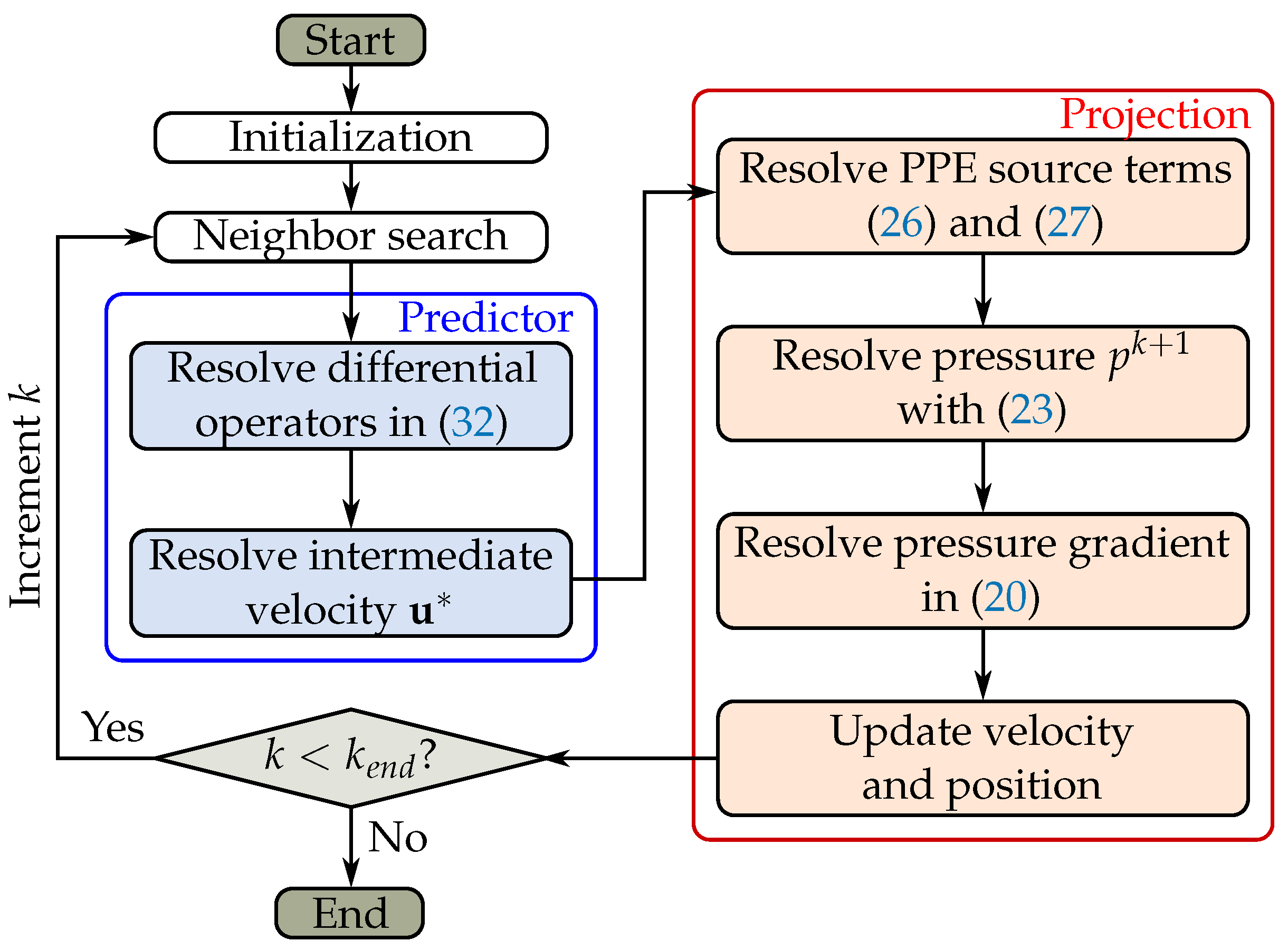
2.6. Solver Overview

This section provides a high-level overview of the numerical method. The control flow of the algorithm is discussed along with a theoretical analysis of the computational cost of the scheme.
Figure 1 shows the process flow diagram of the solver. The only host or central processing unit (CPU) step is the initialization step. This involves the particle generation and setting of the initial conditions for both the fluid and boundary particles. Once initialized, the particle data are copied onto the GPU. A spatial hash map is used to resolve the particle neighbor list by generating a linked list for all particles within a spatial hash. Since the cell size is chosen to be 3 h , each particle iterates over the linked lists of the 3 × 3 × 3 cells in its local neighborhood when building GFD operators.
Once the neighbor list is constructed, the differential operators required for the predictor can be resolved. Since the gradients and Laplacians depend on B and o , this is carried out over two passes of the neighbor list, with the first pass constructing the truncation tensor, offset vector, and pre-truncated gradients and the second constructing the second-order partial derivatives 2 u and κ . By truncating the gradients after their construction, the tensor contraction only needs to be performed once per particle. The predictor step is completed by determining the intermediate velocity.
The projection step starts with another pass over the neighbor list used to construct the PPE source terms. Once completed, the PPE is solved iteratively using a BiCGSTAB solver. A final pass over the neighbor list is used to generate the pressure gradient, which is used to project the velocity onto a divergence-free space. Finally, the particle positions are updated according to the velocity and the particle-shifting scheme in [26]. This process then repeats until the simulation terminates.
It should be mentioned that the process flow only describes the solver itself and not the full framework it is implemented within. As such, supplementary processes such as file writing are not discussed. Although these processes do not contribute to the algorithm’s cost, there is a cost associated with these processes due to the additional device-to-host data transfer they require.
To evaluate the computational cost, here we follow the approach presented in [32,42]. Specifically, the construction of the GFD operators first resolves the pairwise interaction between a particle and one of its neighbors. Each particle then iterates over its neighbor list to add the pairwise interactions and generate the full GFD operator. The summation of pairwise interactions is treated naively by approximating its cost as one FLOP per term.
Table 1 shows the floating-point operations (FLOPS) per pairwise interaction for a simulation in dimension d. It should be noted that this estimate does not include the cost of kernel evaluations and thus implies that this only provides a lower bound on the computational cost. Since gradients are post-multiplied by B , the cost of truncation is also neglected, along with any other post-multiplication. Laplacians do not take into account the cost of constructing the denominator, since this information is already determined when calculating the numerator and is directly reused when resolving the denominator. Furthermore, the cost of matrix multiplication in the BiCGSTAB solver for the PPE is approximated as the cost of constructing the pressure Laplacian.
The computational cost per time step is distributed between one-off GFD operator evaluations and the iterative PPE solver. The one-off operators have a total cost of ( 6 d 2 + 30 d + 18 ) n N , while the PPE requires 2 M ( 3 d + 4 ) n N , with n being the average number of neighboring particles, N being the total number of particles, and M being the average number of iterations for the BiCGSTAB solver. The 2 M factor corresponds to calling two matrix multiplications per iteration. As such, the total computational cost is given as ( 6 d 2 + ( 30 + 6 M ) d + 18 + 8 M ) n N . For the rising bubble simulation of Section 3.2, it was found that the PPE typically requires three iterations to converge. Considering the 4.2 million particles in the simulation, with each having 200 neighbors, 201.6 GFLOPS are required per iteration. The high computational cost makes serial implementation unfeasible, but since the cost is distributed over decoupled pairwise terms, they can be resolved in a massively parallel fashion. This makes multi-CPU or GPU hardware solutions the appropriate choice.
Ultimately, the hardware, energy, and maintenance cost determine what technology is appropriate. At the time of writing, GPUs provide significant benefits in all these categories for massively parallel tasks, thus making them an attractive choice for MLMs in general [43,44,45,46,47].

3. Results and Discussion

Three simulation cases are presented in this work. The first case serves as a verification study of the multiphase method, focusing on the interface and surface tension resolution. For this case, the relaxation of a square droplet is simulated. This case was chosen since the dynamics are completely driven by surface tension and thus serve as a good test case for the surface and force resolution. Comparisons to analytical solutions are provided.
The second case builds on the first by introducing additional physics to the droplet system. By including buoyancy, relative motion between the two fluids is induced. Aside from the surface tension resolution, the surface shear conditions at the multiphase interface must be resolved to recover both the droplet shape and bulk kinematic behavior.
Finally, a high-fidelity simulation of spherical droplet coalescence and break-up is simulated. These simulations highlight the robustness of the scheme when treating large surface deformations and thin film features.
All results presented were obtained from full 3D simulations. The solver is written in C++ and utilizes the NVIDIA CUDA toolkit for parallelization.

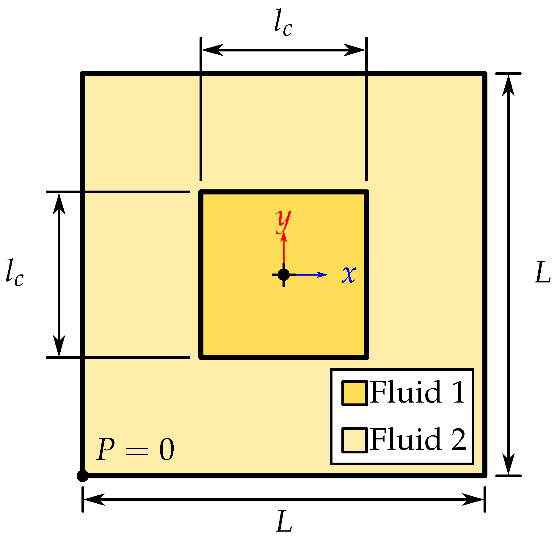
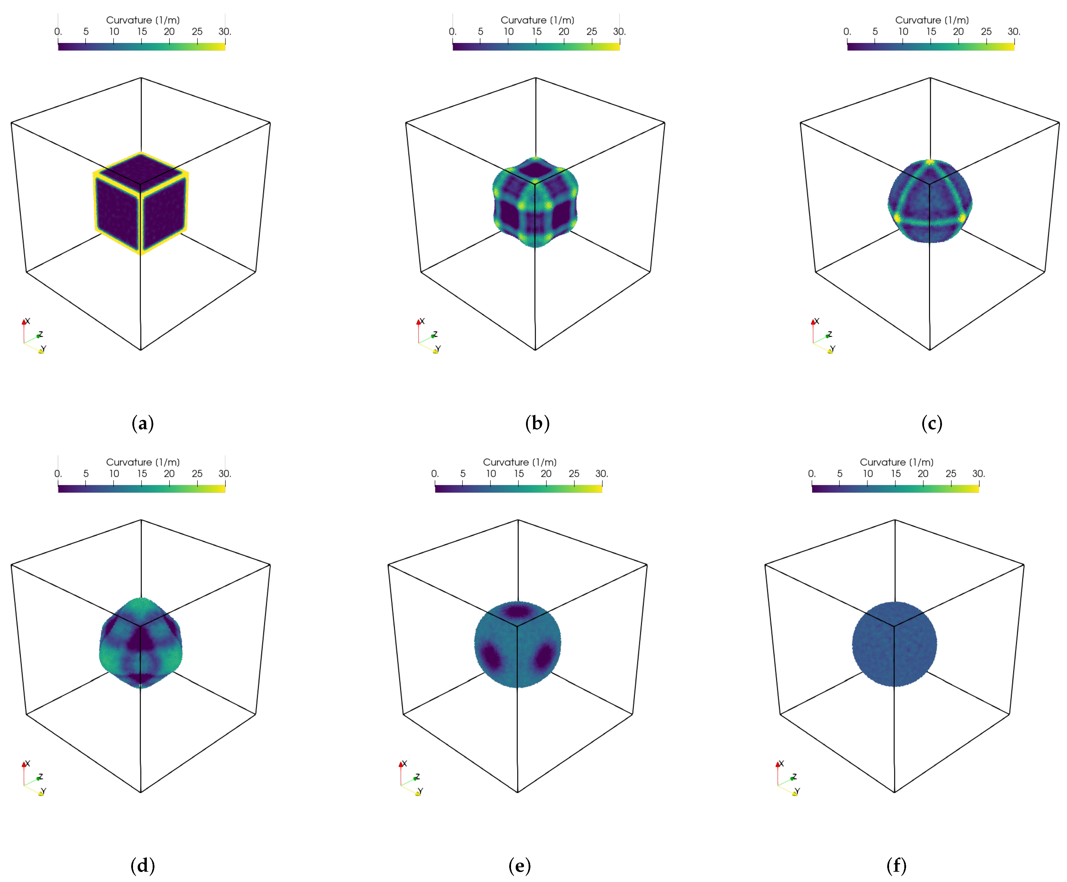
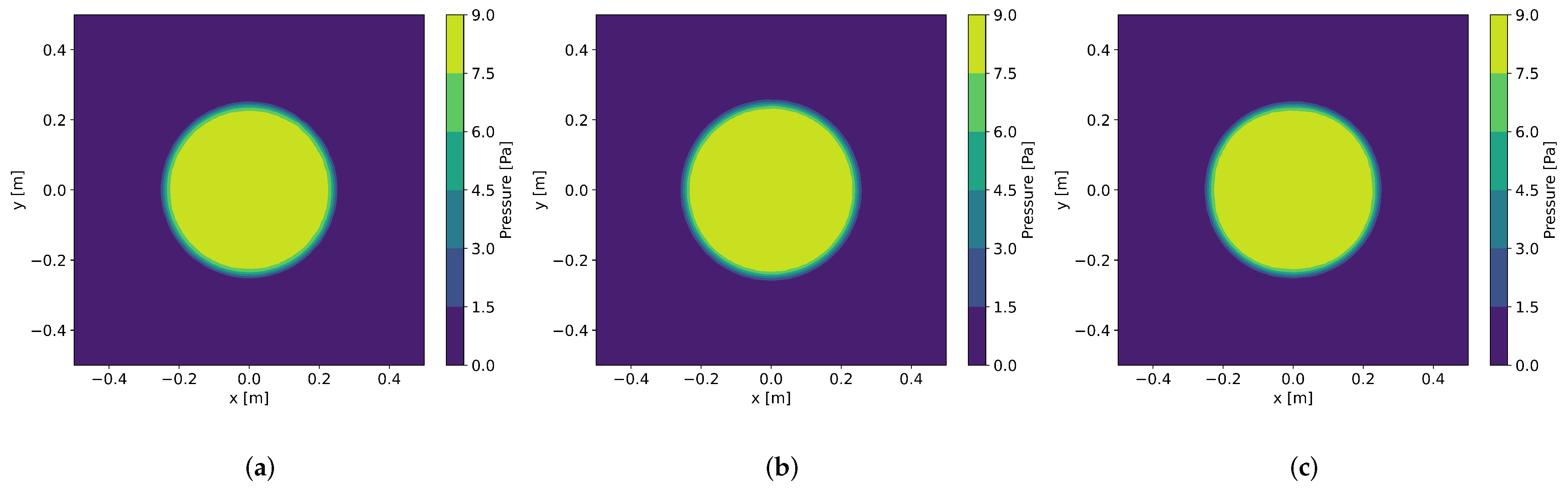
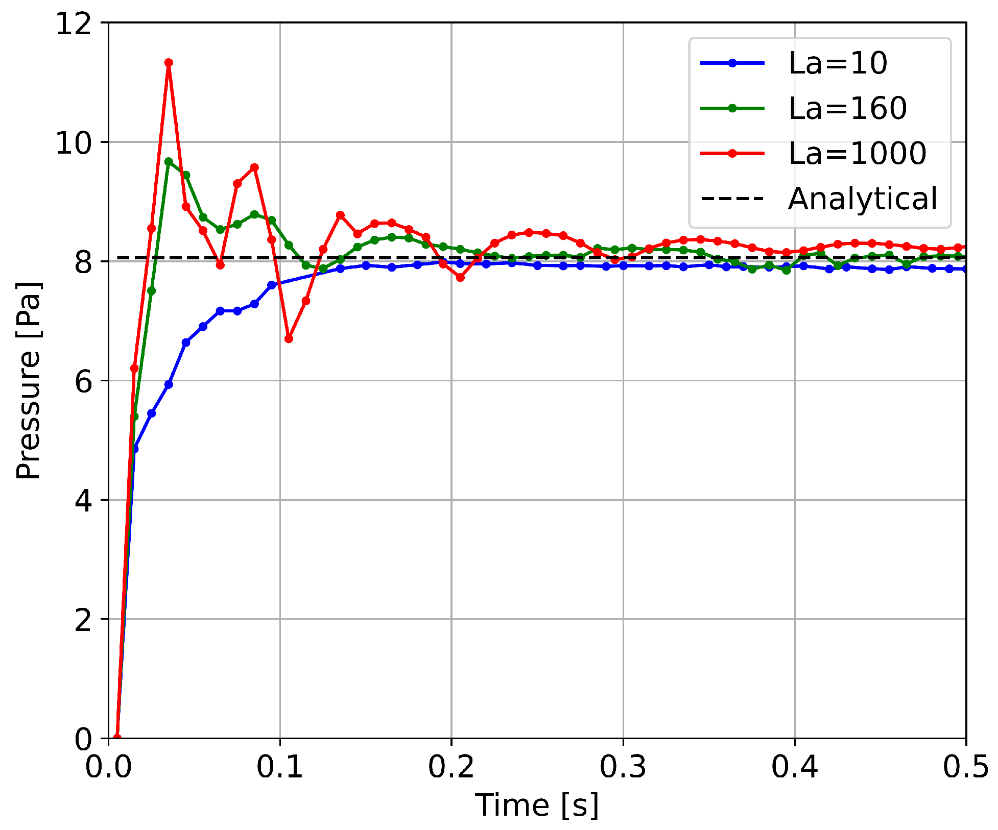
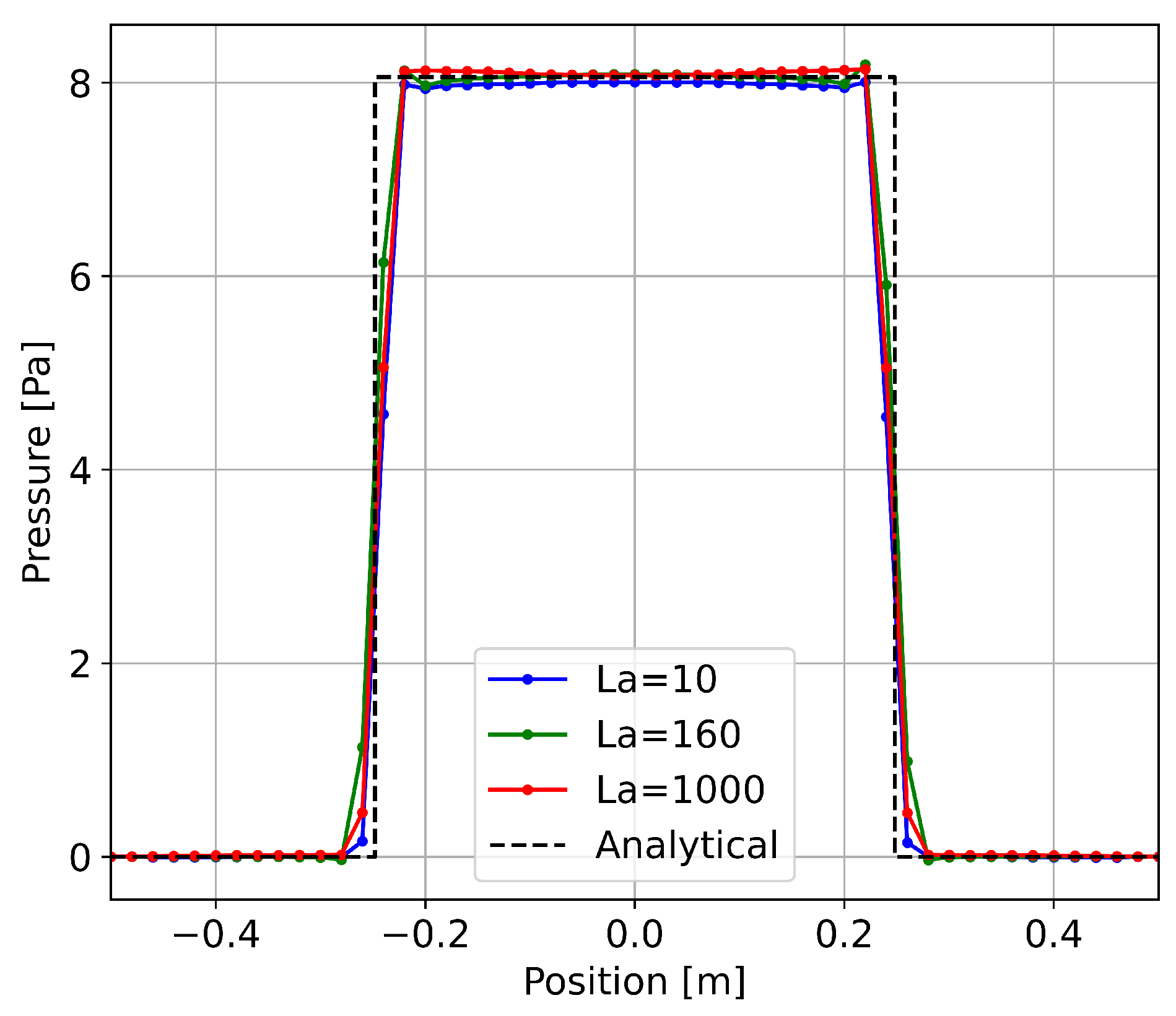
3.1. Square Droplet Relaxation
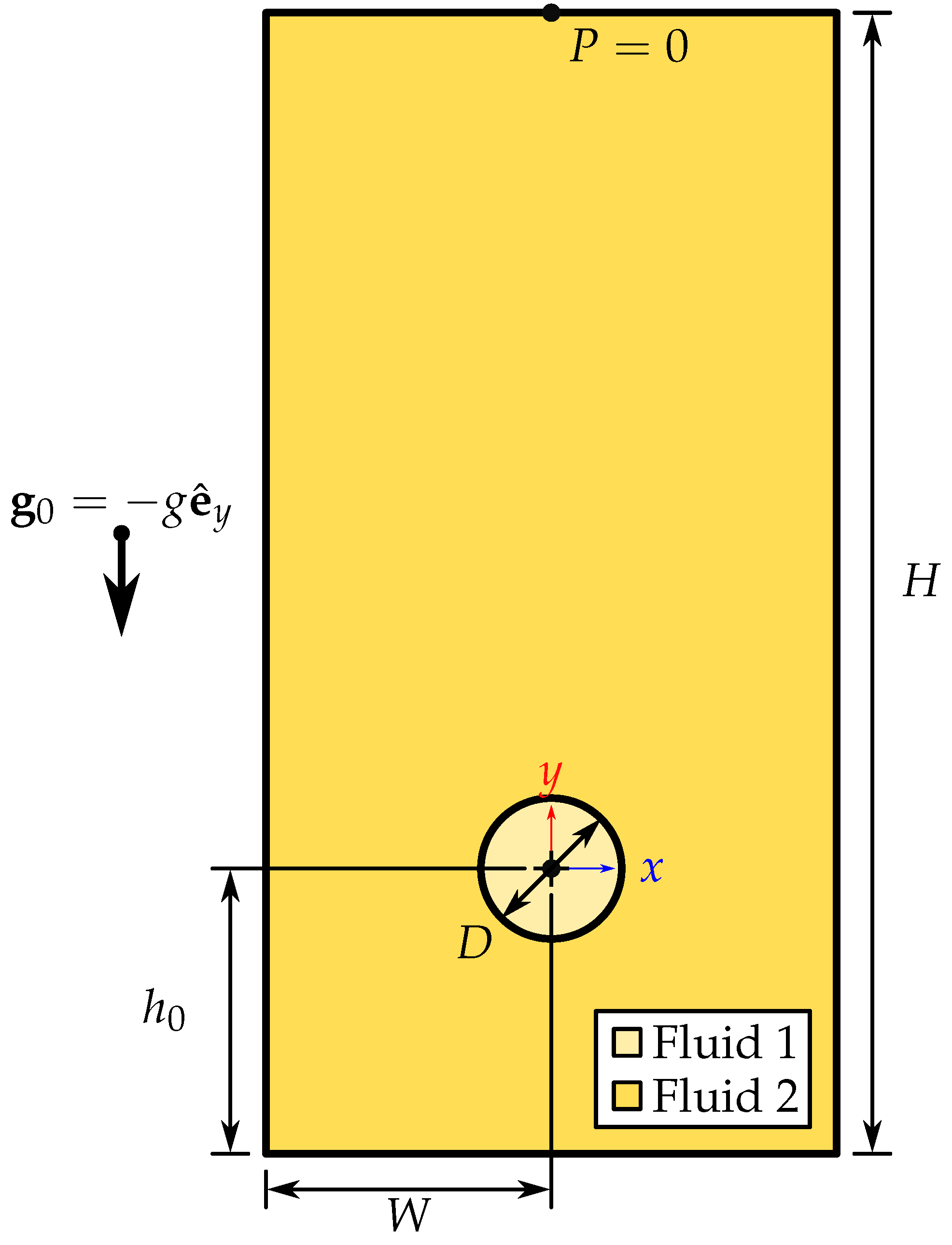
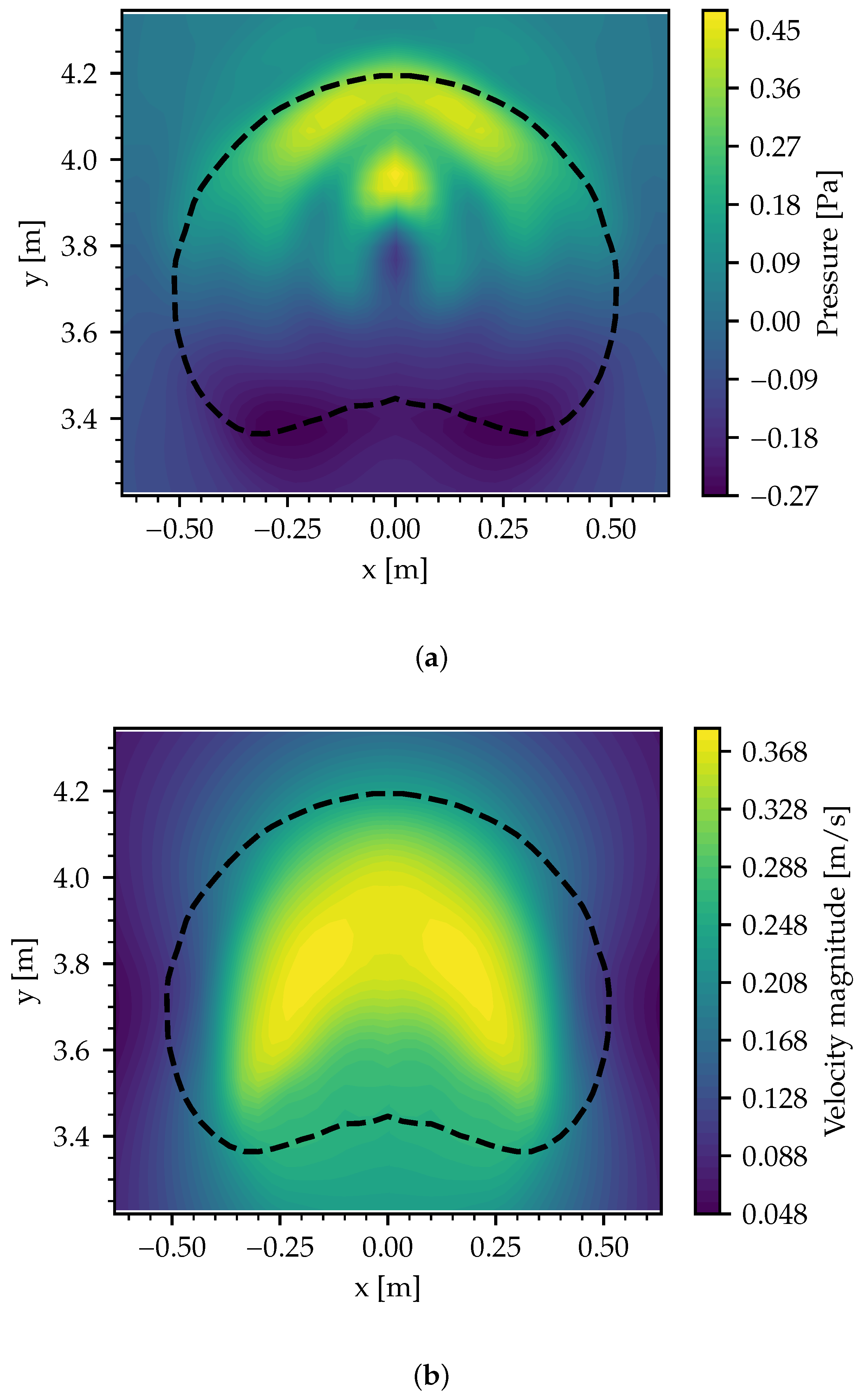
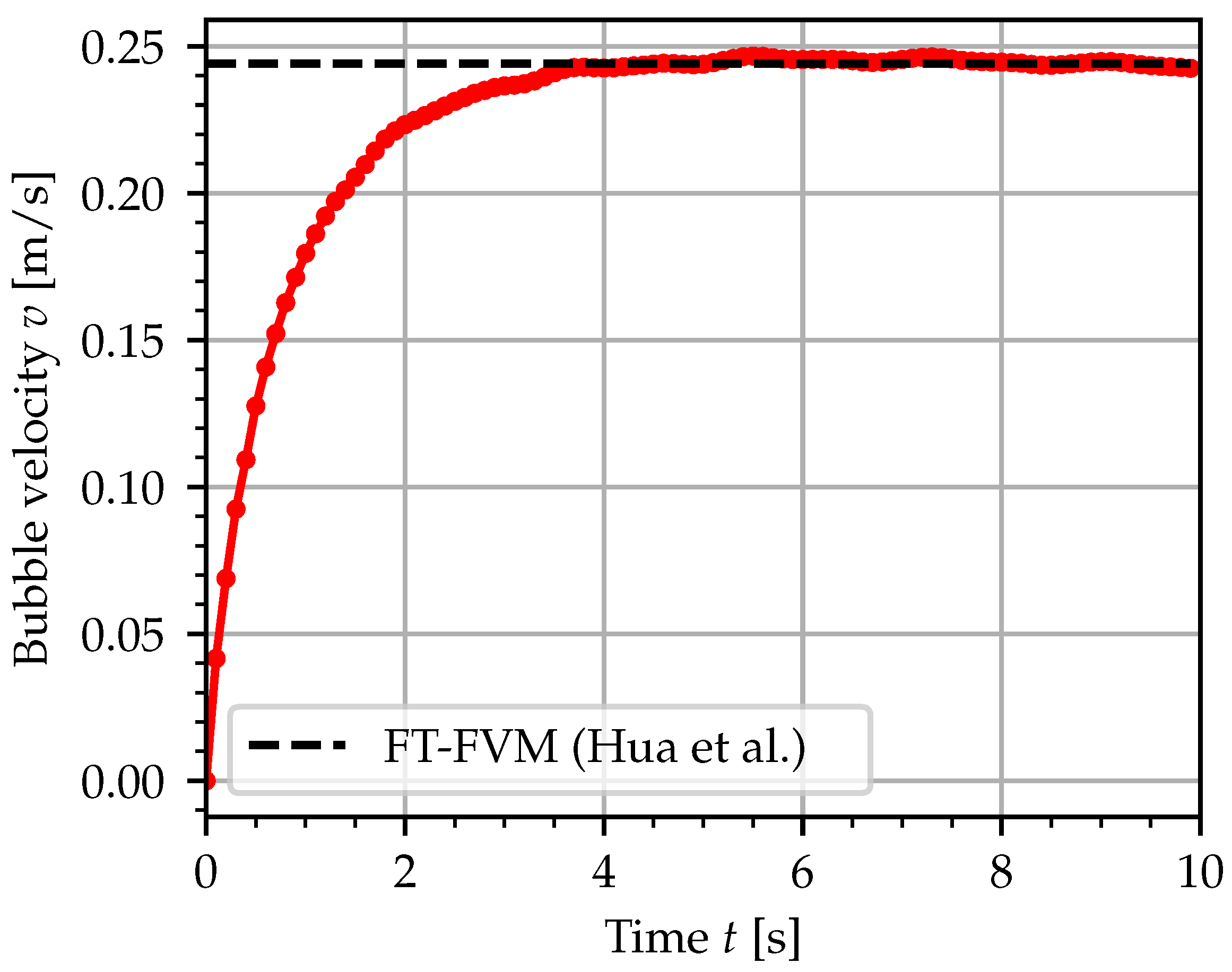
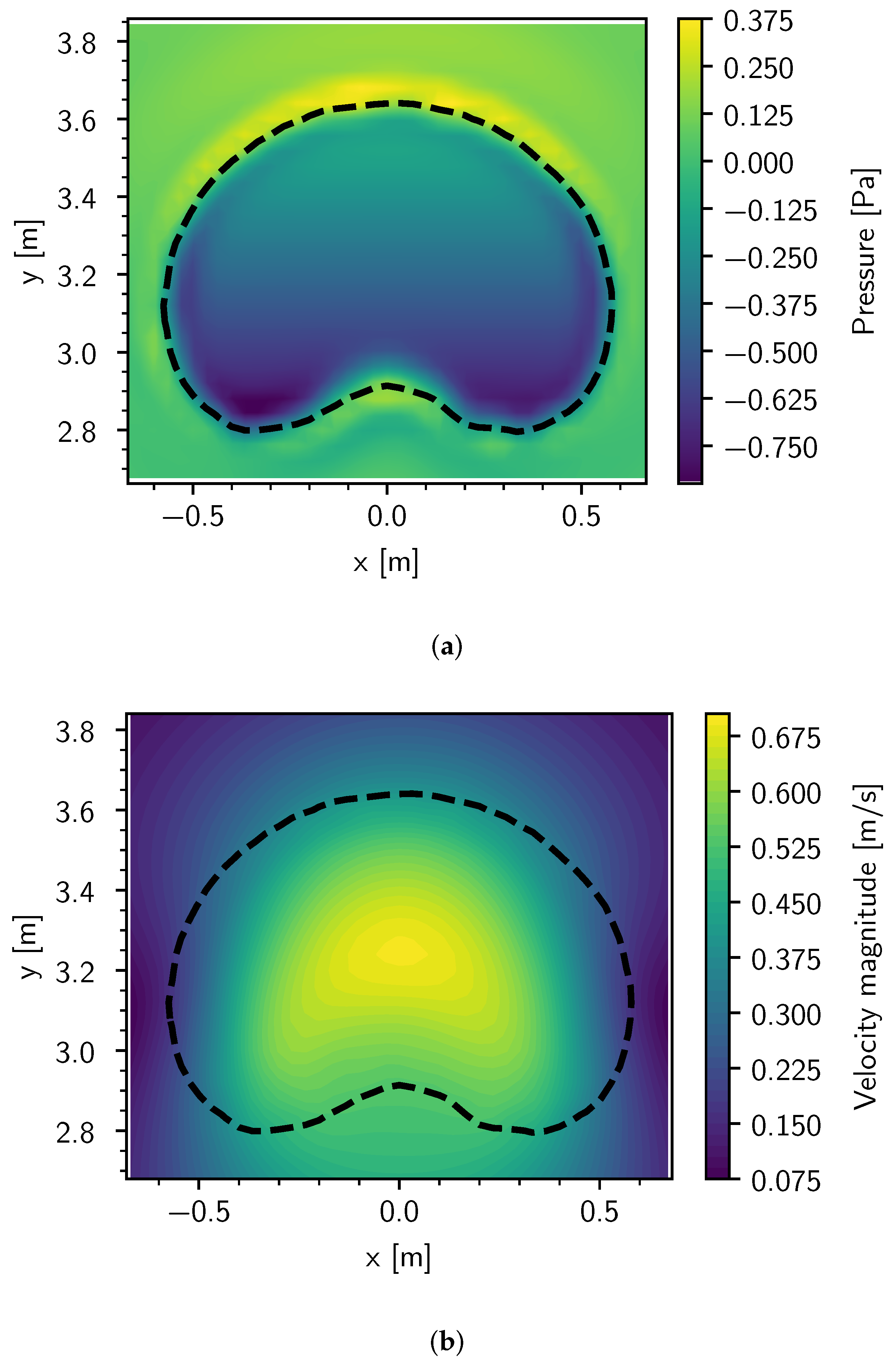
Verification of the surface tension resolution followed the same procedure as that presented in [48]. The case was constructed by initializing a primary fluid inside a cube with sides of a length l c = 0.4 m. An external fluid filled the volume between the primary fluid and a larger cube with sides of a length L = 1 m. A no-slip condition was enforced on all boundary surfaces. A pointwise zero-pressure condition was enforced at ( L / 2 , L / 2 , L / 2 ) , uniquely defining the pressure field. A schematic description of the system is shown in Figure 2.
Surface tension drives the evolution of this multiphase interface. To minimize the interface energy, the interface tends toward a sphere. The internal fluid pressure tends toward a constant value based on the curvature of the sphere and surface tension coefficient given by Δ P = 2 σ / R , with R = l c 3 / 4 π 3 as the spherical droplet radius. All simulations made use of the same l c and σ and thus shared this analytical solution.
Three simulations are performed in this section. A reference simulation with the same non-dimensional parameters as those in [48] is performed. This is followed by two simulations with increasing density ratios. A viscosity ratio of ν 1 : ν 2 = 1:1 was used for all simulations. The simulations were characterized by a Laplace number La = σ l c / ρ 1 ν 1 2 and density ratio ρ 1 : ρ 2 . The material properties and non-dimensional numbers can be seen in Table 2. A particle spacing of δ = L / 100 was used for all simulations, resulting in a 970,000 particle simulation. A support radius of 3 h = 3 δ was used for all simulations.
Figure 3 shows snapshots of the droplet for La = 1000 . As expected, the regions with higher curvature were driven such that the curvature essentially diffused over the surface. The viscosity dampened the flow to produce subsequently smoother interfaces until a spherical droplet was obtained.
Figure 4a–c shows the mid-plane pressure field at time t = 1 s for all three cases. When matching the analytical solution’s prediction, the pressure field is uniform over the spherical droplet. Figure 5 shows the evolution of the averaged pressure difference between the two phases for the three cases. As expected, the relaxation time increased with a decrease in viscosity. However, since the droplet volume and surface tension coefficient were fixed over the simulations, each case oscillated around P . The steady state pressure along the centerline in the x direction is presented in Figure 6. The integrated error for La = 10 , La = 160 , and La = 1000 was 2.23%, 1.64%, and 1.56%, respectively. As highlighted by Figure 6, this error was mainly due to the pressure discontinuity being resolved by the CSF over a finite width.

3.2. Rising Bubble

This section presents the proposed scheme’s handling of a bubble rising in a denser and more viscous fluid. The results are compared against the FT-FVM of Hua et al. [3] and the axisymmetric WCSPH of Li et al. [49].
Following [3], gravity was only applied to the bubble. As such, the body force used in this section is given by ρ g = ( ρ ρ 2 ) g 0 , where ρ 2 is the outer fluid’s density and g 0 is the acceleration due to gravity. It should be noted that the density used in the body force was the unmodified density of the phase before smoothing.
The full 3D system was simulated. The bubble was initialized in a spherical domain, while the dense fluid was initialized in the remaining volume between the bubble and a cylindrical wall with full-slip conditions. No-slip conditions were enforced on the cylinder caps. A pointwise zero-pressure condition was enforced on the top cap at ( 0 , H h 0 , 0 ) . A schematic description of the system can be seen in Figure 7. The geometry was configured with H = 24 D , W = 2 D , h 0 = 2 D , and D = 1 m, and gravity was set to g = 1.0 m / s 2 .
The flow was categorized by the density ratio ρ 1 : ρ 2 , the viscosity ratio μ 1 : μ 2 , the Reynolds number Re = U c D / ν 2 , and the Bond number B o = ρ 2 D U c 2 / σ , with U c = g D as the characteristic velocity. The material properties and non-dimensional numbers for this system can be seen in Table 3. A support radius of 3 h = 3.6 δ and an initial particle spacing of δ = D / 32 was used for this simulation. As such, 4.2 million particles were used to discretize the fluid domain. A low and high density ratio case are considered in this section.
The pressure and velocity fields for Case 1 at t = 8.1 s can be seen in Figure 8a,b, respectively. As expected, a high-pressure zone developed on the leading surface, while a low-pressure region was observed in the bubble’s wake. The lower viscosity of the bubble resulted in a high internal velocity that decayed toward the multiphase interface.
Figure 9 compares the steady state bubble shape to the results of both [3,49]. A qualitatively good agreement between both shapes was observed. However, it can be noticed that both the FVM and WCSPH results predicted slightly wider bubbles at 1.09 m and 1.07 m, respectively, compared with the current method’s predicted width of 1.03 m. Interestingly, although the trailing surface lied between the FVM and WCSPH results, this scheme predicted a shape with pronounced lobes on the trailing surface similar to that of the FVM results.
Figure 10 presents the bulk behavior of the bubble over time. The bubble’s average velocity is shown. The velocity was compared against the steady state value obtained in [3]. Again, good agreement with the FVM results is shown. It should be noted that unlike in [49], the velocity monotonically increased up to its steady state conditions, after which small fluctuations could be noticed. This was due to gravity only being applied to the bubble, thus ignoring the effects of the dense phase’s pressure field evolving to include hydrostatic conditions. Furthermore, the non-physical high-frequency terms in the bubble’s bulk velocity obtained in [49] were not generated by the current scheme. This was due to the incompressible model resolving the pressure at a global level and thus not generating the high-frequency pressure oscillation typical of the WC mass–momentum coupling model.
As with Case 1, the steady state pressure and velocity fields around the bubble can be seen in Figure 11a,b, respectively. The effects of the high-density ratio were especially prevalent in the pressure field. While the pressure difference across the bubble was similar to the low density ratio case, a significant pressure jump over the interface can be seen. This led to the bubble pressure being lower than the external pressure field.
The evolution of the bubble’s vertical velocity was compared to the results of Hua et al. [3]. These results can be seen in Figure 12. A good correlation between the results was obtained, but it was found that the bubble accelerated slightly faster early in the simulation. Slight fluctuations in the vertical velocity can also be seen before the bubble settled into its steady state condition.

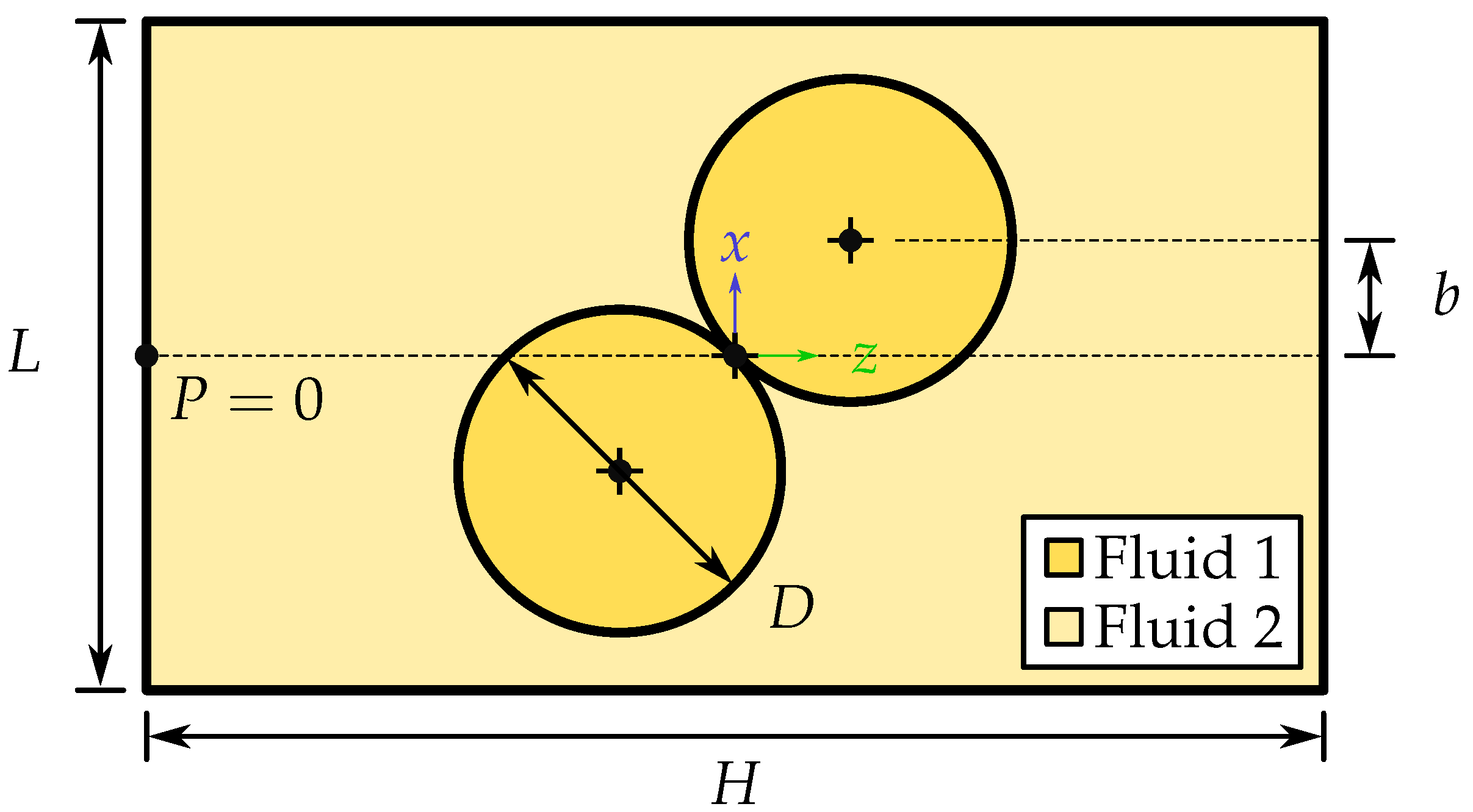
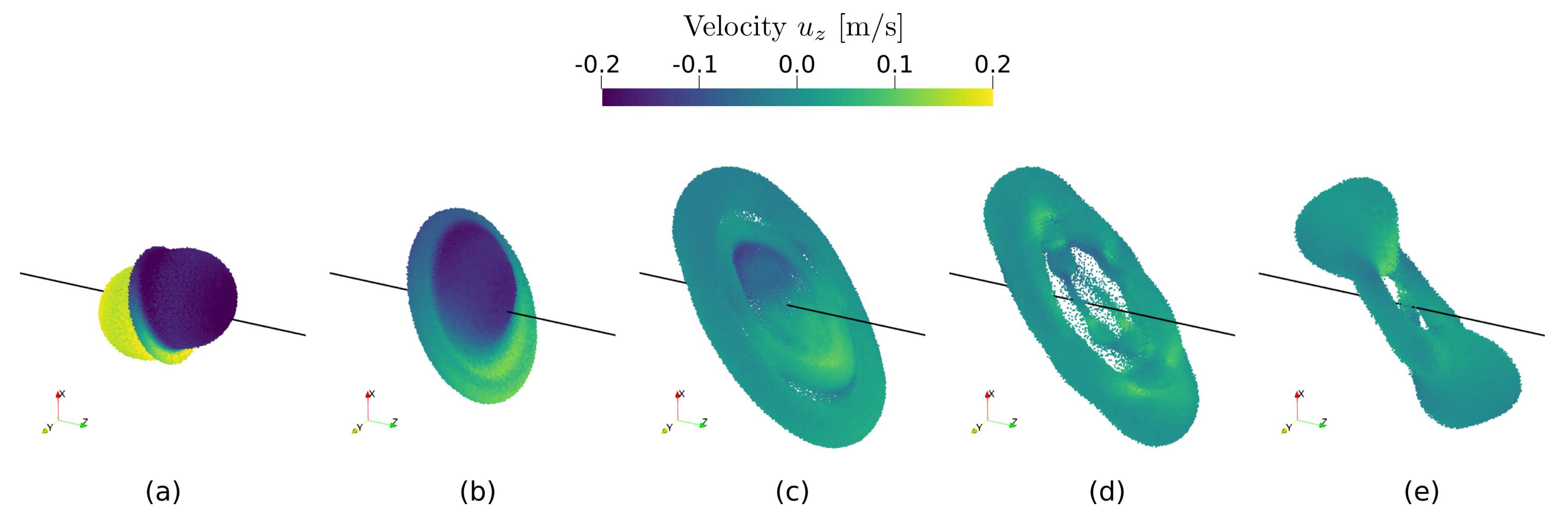
3.3. Colliding Droplets

The final set of simulations presents the behavior of binary droplets interacting. The purpose of this section is to demonstrate the scheme’s behavior when dealing with two distinct multiphase mechanisms, namely coalescence and break-up.
The geometry shown in Figure 13 is used in all cases. Two droplets, each with a diameter D = 1 m, were initialized with an offset of b = 0.135 m away from the cylindrical domain’s centerline. The length of the cylinder was set to H = 4 D , and the diameter was given by L = 4 D . Full-slip conditions were applied to all domain surfaces. The droplets were initialized with a relative velocity of U r = 0.5 m / s .
The cases were constructed to investigate the scheme’s response over several flow regimes characterized by the Reynolds number Re = ρ 1 U r D / μ 1 and Weber number We = ρ 1 U r 2 D / σ . High density ratio cases were explored with both low and high We values to show the effects of surface tension. With high density ratio systems being more resistant to break-up, a low density ratio case was also simulated at high We values. Table 4 shows the fluid material properties of the cases along with their non-dimensional numbers. A support radius of 3 h = 3.6 δ and an initial particle spacing of δ = D / 48 were used, leading to simulations with 5.4 million particles each.
The 3D evolution of the droplet particles can be seen in Figure 14, Figure 15 and Figure 16. These results are colored by their z-velocities, with the black line indicating the cylinder centerline. Qualitatively distinct behavior was observed between the systems. Specifically, the large surface tension of the low We case was sufficient to prevent fluid separation after the droplets coalesced. As a result, the net angular momentum of the system resulted in the combined droplet rotating about the system’s center. Large deformations in the interface were observed initially but were soon dampened out by viscous effects.
Alternatively, the restoring surface tension forces of the high We cases were not large enough to overcome the momentum of the droplets. Considering the high density ratio case, the droplets can be seen to have initially merged, followed by large surface deformation, leading to the formation of a torus seen at t = 11.25 s. It should be noted that a thin film formed in the center of the torus. Once this film thickness reduced beyond the GFD particle diameter, a numerical rupture took place, and the fluid that was originally part of the film recombined to form a separate structure. Ultimately, the surface tension pulled the torus inward and created two growing droplets connected by the shrinking arms of the torus.
Similar behavior can be seen between the high and low density ratio case initially, with both cases producing a thin film structure, but as the system progressed, it can be seen that the generated torus remained intact over the simulation period. Furthermore, although a thin film structure formed again, the film evolved to form a second smaller torus separate from the main structure. This secondary torus eventually experienced further break-up and formed smaller droplets. This behavior is qualitatively similar to a similar case investigated in [2].
The mean velocity moment of the droplets around the computational domain’s centroid was used to quantitatively compare the systems:
t = 1 | I D | i I D r i × u i ,
where I D is the set indexing of all particles belonging to the droplet and | I D | is the size of I D . Due to particle spacing remaining uniform over the simulations, the volume associated with each particle was approximately uniform and constant. As such, t measured the angular momentum of the droplets normalized by mass. Figure 17 shows the evolution of the velocity moment around the y axis t y .
The low density ratio case lost energy much faster than the high density ratio case. This was expected since, in the low density ratio case, the droplets acted against an external fluid of a similar density, as opposed to the high density ratio case, where the droplets carried most of the system’s energy. Fluctuations in the velocity moment can be seen between t = 10 s and t = 15 s for the low density ratio case. This coincided with the rupture of the film structure and the formation of the internal torus.
When comparing the We = 8 and We = 180 cases, the high-We case damped out faster despite having a higher Re. This can be explained by the differences in the fluid motion induced by the surface tension. When considering the initial collision, the We = 8 case did damp out faster during this period, but once the droplets coalesced, they started rotating as a single droplet around the domain’s center, with any further dampening being almost exclusively due to momentum diffusion due to shear at the surface interface. In contrast, the We = 180 case had a more dynamic response, providing more modes for momentum diffusion. Furthermore, this case was subject to significant surface formation, which served as an additional mechanism to store the system’s energy.

4. Conclusions

This work presented a GFD scheme for incompressible multiphase flow that is suitable for high density ratios. This was achieved by introducing a dampening term in the predictor step based on a Riemann solver pressure gradient correction term that resulted in the dampening of high-frequency responses arising at multiphase interfaces. This allowed the cost-effective, first-order accurate GFD differential operators to be used in incompressible multiphase environments. Furthermore, the dampening scheme only requires the resolution of one additional gradient operator. This keeps the complexity and the incurred computational cost low.
The scheme was verified against analytical and numerical solutions. When simulating the relaxation of a square droplet, the accuracy of the steady state solution was comparable between all cases. It was found that the primary source of errors was the CSF model introducing a finite pressure gradient over the interface. Good agreement with the analytical solution was shown outside the interface’s support domain.
Similarly, good agreement between the FVM and SPH results was found when simulating a bubble rising in a dense fluid. Although slight discrepancies were obtained in the shape of the bubble, this work predicted a bubble shape similar to both the FVM and SPH results. Furthermore, the vertical velocity of the bubble closely matched the FVM results as well.
Finally, the collision of two droplets was numerically investigated as well. The scheme’s ability to treat both low and high density ratios was shown. Furthermore, it was shown that the scheme could handle a wide range of flow regimes as well. The scheme’s treatment of thin fluid structures was highlighted and shown to be stable, even to the point of numerical rupture for both the high and low density ratio cases. Although the scheme was shown to be robust in the presence of thin fluid structures, a future study is recommended to validate the collision results and to further investigate the accuracy of the dynamics of the thin film structures.
The cases investigated in this work only considered slow surface dynamics. In more dynamic environments, it is expected that the dampening introduced at the interface will smooth out the response, leading to an underprediction of the surface shear, especially for high viscosity ratio cases. As such, the applicability of this scheme to violent surface dynamics should be explored further to assess the significance of this behavior.

Author Contributions

Conceptualization, methodology, software, formal analysis, investigation, writing—original draft preparation, and visualization, J.C.J.; conceptualization, methodology, investigation, writing—review and editing, and supervision, D.N.W.; resources, writing—review and editing, and supervision, P.P. All authors have read and agreed to the published version of this manuscript.

Funding

The authors wish to express their gratitude for the financial support provided by the University of Pretoria Co-Funding Postdoctoral Fellowship Programme.

Conflicts of Interest

The authors declare no conflict of interest.

References

  1. Brackbill, J.; Kothe, D.; Zemach, C. A continuum method for modeling surface tension. J. Comput. Phys. 1992, 100, 335–354. [Google Scholar] [CrossRef]
  2. Lafaurie, B.; Nardone, C.; Scardovelli, R.; Zaleski, S.; Zanetti, G. Modelling Merging and Fragmentation in Multiphase Flows with SURFER. J. Comput. Phys. 1994, 113, 134–147. [Google Scholar] [CrossRef]
  3. Hua, J.; Lou, J. Numerical simulation of bubble rising in viscous liquid. J. Comput. Phys. 2007, 222, 769–795. [Google Scholar] [CrossRef]
  4. Hu, X.; Adams, N. A multi-phase SPH method for macroscopic and mesoscopic flows. J. Comput. Phys. 2006, 213, 844–861. [Google Scholar] [CrossRef]
  5. Douillet-Grellier, T.; Leclaire, S.; Vidal, D.; Bertrand, F.; De Vuyst, F. Comparison of multiphase SPH and LBM approaches for the simulation of intermittent flows. Comput. Part. Mech. 2019, 6, 695–720. [Google Scholar] [CrossRef] [Green Version]
  6. Adami, S.; Hu, X.Y.; Adams, N.A. A new surface-tension formulation for multi-phase SPH using a reproducing divergence approximation. J. Comput. Phys. 2010, 229, 5011–5021. [Google Scholar] [CrossRef]
  7. Zhang, A.; Sun, P.; Ming, F. An SPH modeling of bubble rising and coalescing in three dimensions. Comput. Methods Appl. Mech. Eng. 2015, 294, 189–209. [Google Scholar] [CrossRef]
  8. Ming, F.R.; Sun, P.N.; Zhang, A.M. Numerical investigation of rising bubbles bursting at a free surface through a multiphase SPH model. Meccanica 2017, 52, 2665–2684. [Google Scholar] [CrossRef]
  9. Yan, J.; Li, S.; Zhang, A.M.; Kan, X.; Sun, P.N. Updated Lagrangian Particle Hydrodynamics (ULPH) modeling and simulation of multiphase flows. J. Comput. Phys. 2019, 393, 406–437. [Google Scholar] [CrossRef]
  10. Zainali, A.; Tofighi, N.; Shadloo, M.S.; Yildiz, M. Numerical investigation of Newtonian and non-Newtonian multiphase flows using ISPH method. Comput. Methods Appl. Mech. Eng. 2013, 254, 99–113. [Google Scholar] [CrossRef]
  11. Szewc, K.; Pozorski, J.; Minier, J.P. Spurious interface fragmentation in multiphase SPH. Int. J. Numer. Methods Eng. 2015, 103, 625–649. [Google Scholar] [CrossRef]
  12. Yeganehdoust, F.; Yaghoubi, M.; Emdad, H.; Ordoubadi, M. Numerical study of multiphase droplet dynamics and contact angles by smoothed particle hydrodynamics. Appl. Math. Model. 2016, 40, 8493–8512. [Google Scholar] [CrossRef]
  13. Yang, L.; Rakhsha, M.; Hu, W.; Negrut, D. A consistent multiphase flow model with a generalized particle shifting scheme resolved via incompressible SPH. J. Comput. Phys. 2022, 458, 111079. [Google Scholar] [CrossRef]
  14. Muradoglu, M.; Tryggvason, G. Simulations of soluble surfactants in 3D multiphase flow. J. Comput. Phys. 2014, 274, 737–757. [Google Scholar] [CrossRef]
  15. Colagrossi, A.; Landrini, M. Numerical simulation of interfacial flows by smoothed particle hydrodynamics. J. Comput. Phys. 2003, 191, 448–475. [Google Scholar] [CrossRef]
  16. Meng, Z.F.; Wang, P.P.; Zhang, A.M.; Ming, F.R.; Sun, P.N. A multiphase SPH model based on Roe’s approximate Riemann solver for hydraulic flows with complex interface. Comput. Methods Appl. Mech. Eng. 2020, 365, 112999. [Google Scholar] [CrossRef]
  17. Yang, Q.; Xu, F.; Yang, Y.; Wang, L. A multi-phase SPH model based on Riemann solvers for simulation of jet breakup. Eng. Anal. Bound. Elem. 2020, 111, 134–147. [Google Scholar] [CrossRef]
  18. Cheng, H.; Liu, Y.; Ming, F.; Sun, P. Investigation on the bouncing and coalescence behaviors of bubble pairs based on an improved APR-SPH method. Ocean. Eng. 2022, 255, 111401. [Google Scholar] [CrossRef]
  19. Chen, Z.; Zong, Z.; Liu, M.; Zou, L.; Li, H.; Shu, C. An SPH model for multiphase flows with complex interfaces and large density differences. J. Comput. Phys. 2015, 283, 169–188. [Google Scholar] [CrossRef]
  20. Zheng, B.; Chen, Z. A multiphase smoothed particle hydrodynamics model with lower numerical diffusion. J. Comput. Phys. 2019, 382, 177–201. [Google Scholar] [CrossRef]
  21. Rezavand, M.; Zhang, C.; Hu, X. A weakly compressible SPH method for violent multi-phase flows with high density ratio. J. Comput. Phys. 2020, 402, 109092. [Google Scholar] [CrossRef] [Green Version]
  22. Vahabi, M.; Kamkari, B. Simulating gas bubble shape during its rise in a confined polymeric solution by WC-SPH. Eur. J. Mech.-B/Fluids 2019, 75, 1–14. [Google Scholar] [CrossRef]
  23. He, F.; Zhang, H.; Huang, C.; Liu, M. A stable SPH model with large CFL numbers for multi-phase flows with large density ratios. J. Comput. Phys. 2022, 453, 110944. [Google Scholar] [CrossRef]
  24. Tong, M.; Browne, D.J. An incompressible multi-phase smoothed particle hydrodynamics (SPH) method for modelling thermocapillary flow. Int. J. Heat Mass Transf. 2014, 73, 284–292. [Google Scholar] [CrossRef]
  25. Cummins, S.J.; Rudman, M. An SPH Projection Method. J. Comput. Phys. 1999, 152, 584–607. [Google Scholar] [CrossRef]
  26. Xu, R.; Stansby, P.; Laurence, D. Accuracy and stability in incompressible SPH (ISPH) based on the projection method and a new approach. J. Comput. Phys. 2009, 228, 6703–6725. [Google Scholar] [CrossRef]
  27. Grenier, N.; Antuono, M.; Colagrossi, A.; Le Touzé, D.; Alessandrini, B. An Hamiltonian interface SPH formulation for multi-fluid and free surface flows. J. Comput. Phys. 2009, 228, 8380–8393. [Google Scholar] [CrossRef]
  28. Rezavand, M.; Taeibi-Rahni, M.; Rauch, W. An ISPH scheme for numerical simulation of multiphase flows with complex interfaces and high density ratios. Comput. Math. Appl. 2018, 75, 2658–2677. [Google Scholar] [CrossRef]
  29. Xu, Y.; Yang, G.; Zhu, Y.; Hu, D. A coupled SPH–FVM method for simulating incompressible interfacial flows with large density difference. Eng. Anal. Bound. Elem. 2021, 128, 227–243. [Google Scholar] [CrossRef]
  30. Zheng, B.; Sun, L.; Yu, P. A novel interface method for two-dimensional multiphase SPH: Interface detection and surface tension formulation. J. Comput. Phys. 2021, 431, 110119. [Google Scholar] [CrossRef]
  31. Geara, S.; Martin, S.; Adami, S.; Petry, W.; Allenou, J.; Stepnik, B.; Bonnefoy, O. A new SPH density formulation for 3D free-surface flows. Comput. Fluids 2022, 232, 105193. [Google Scholar] [CrossRef]
  32. Joubert, J.C.; Wilke, D.N.; Govender, N.; Pizette, P.; Basic, J.; Abriak, N.E. Boundary condition enforcement for renormalised weakly compressible meshless Lagrangian methods. Eng. Anal. Bound. Elem. 2021, 130, 332–351. [Google Scholar] [CrossRef]
  33. Basic, J.; Blagojevic, B.; Andrun, M.; Degiuli, N. A Lagrangian Finite Difference Method for Sloshing: Simulations and Comparison with Experiments. In Proceedings of the Twenty-Ninth International Ocean and Polar Engineering Conference, Honolulu, HI, USA, 11–16 October 2019; pp. 3412–3418. [Google Scholar]
  34. Joubert, J.C.; Wilke, D.N.; Pizette, P. On the momentum diffusion over multiphase surfaces with meshless methods. arXiv 2023, arXiv:2303.09978. [Google Scholar]
  35. Morris, J.P.; Fox, P.J.; Zhu, Y. Modeling low Reynolds number incompressible flows using SPH. J. Comput. Phys. 1997, 136, 214–226. [Google Scholar] [CrossRef]
  36. Lanson, N.; Vila, J.P. Renormalized Meshfree Schemes I: Consistency, Stability, and Hybrid Methods for Conservation Laws. SIAM J. Numer. Anal. 2008, 46, 1912–1934. [Google Scholar] [CrossRef]
  37. Lanson, N.; Vila, J.P. Renormalized Meshfree Schemes II: Convergence for Scalar Conservation Laws. SIAM J. Numer. Anal. 2008, 46, 1935–1964. [Google Scholar] [CrossRef]
  38. Basic, J.; Degiuli, N.; Ban, D. A class of renormalised meshless Laplacians for boundary value problems. J. Comput. Phys. 2018, 354, 269–287. [Google Scholar] [CrossRef]
  39. Inutsuka, S.-I. Reformulation of Smoothed Particle Hydrodynamics with Riemann Solver. J. Comput. Phys. 2002, 179, 238–267. [Google Scholar] [CrossRef] [Green Version]
  40. Puri, K.; Ramachandran, P. Approximate Riemann solvers for the Godunov SPH (GSPH). J. Comput. Phys. 2014, 270, 432–458. [Google Scholar] [CrossRef]
  41. Zhang, C.; Hu, X.; Adams, N. A weakly compressible SPH method based on a low-dissipation Riemann solver. J. Comput. Phys. 2017, 335, 605–620. [Google Scholar] [CrossRef]
  42. Mao, Z.; Liu, G.R. A Lagrangian gradient smoothing method for solid-flow problems using simplicial mesh. Int. J. Numer. Methods Eng. 2018, 113, 858–890. [Google Scholar] [CrossRef]
  43. Xia, X.; Liang, Q. A GPU-accelerated smoothed particle hydrodynamics (SPH) model for the shallow water equations. Environ. Model. Softw. 2016, 75, 28–43. [Google Scholar] [CrossRef]
  44. Zhan, L.; Peng, C.; Zhang, B.; Wu, W. A stabilized TL–WC SPH approach with GPU acceleration for three-dimensional fluid–structure interaction. J. Fluids Struct. 2019, 86, 329–353. [Google Scholar] [CrossRef]
  45. Afrasiabi, M.; Klippel, H.; Roethlin, M.; Wegener, K. An improved thermal model for SPH metal cutting simulations on GPU. Appl. Math. Model. 2021, 100, 728–750. [Google Scholar] [CrossRef]
  46. Zhang, H.; Zhang, Z.; He, F.; Liu, M. Numerical investigation on the water entry of a 3D circular cylinder based on a GPU-accelerated SPH method. Eur. J. Mech.-B/Fluids 2022, 94, 1–16. [Google Scholar] [CrossRef]
  47. Mao, Y.; Kong, Y.; Guan, M. GPU-accelerated SPH modeling of flow-driven sediment erosion with different rheological models and yield criteria. Powder Technol. 2022, 412, 118015. [Google Scholar] [CrossRef]
  48. Wen, X.; Zhao, W.; Wan, D. A multiphase MPS method for bubbly flows with complex interfaces. Ocean. Eng. 2021, 238, 109743. [Google Scholar] [CrossRef]
  49. Li, M.K.; Zhang, A.M.; Ming, F.R.; Sun, P.N.; Peng, Y.X. An axisymmetric multiphase SPH model for the simulation of rising bubble. Comput. Methods Appl. Mech. Eng. 2020, 366, 113039. [Google Scholar] [CrossRef]
Figure 1. Flow diagram of the numerical scheme.
Mca 28 00051 g001
Figure 2. Schematic description of the square droplet case.
Mca 28 00051 g002
Figure 3. Droplet curvature for La = 1000 at (a) t = 0 s, (b) t = 0.015 s, (c) t = 0.030 s, (d) t = 0.045 s, (e) t = 0.100 s, and (f) t = 0.500 s.
Mca 28 00051 g003
Figure 4. Mid-plane pressure field at t = 1 s for (a) La = 10 , (b) La = 160 , and (c) La = 1000 .
Mca 28 00051 g004
Figure 5. Time evolution of the pressure difference between fluid phases.
Mca 28 00051 g005
Figure 6. Steady state fluid pressure along the centerline in the x direction.
Mca 28 00051 g006
Figure 7. Schematic description of the rising bubble case.
Mca 28 00051 g007
Figure 8. Mid-plane continuum results for the rising bubble in Case 1, showing (a) the pressure field and (b) the velocity field at t = 8.1 s.
Mca 28 00051 g008
Figure 9. Terminal bubble shape compared against [3,49].
Mca 28 00051 g009
Figure 10. Bubble velocity evolution compared against the terminal velocity in [3].
Mca 28 00051 g010
Figure 11. Mid-plane continuum results for the rising bubble Case 2, showing (a) the pressure field and (b) the velocity field at t = 4.0 s.
Mca 28 00051 g011
Figure 12. Bubble velocity evolution compared against the results in [3].
Mca 28 00051 g012
Figure 13. Schematic description of the colliding droplets case.
Mca 28 00051 g013
Figure 14. Droplet collision for Re = 250, We = 8, and ρ 1 : ρ 2 = 1000 : 1 at (a) t = 0.25 s, (b) t = 1 s, (c) t = 2.75 s, (d) t = 5 s, and (e) t = 7.5 s.
Mca 28 00051 g014
Figure 15. Droplet collision for Re = 550, We = 180, and ρ 1 : ρ 2 = 1000 : 1 at (a) t = 1 s, (b) t = 3.25 s, (c) t = 11.25 s, (d) t = 15 s, and (e) t = 22.5 s.
Mca 28 00051 g015
Figure 16. Droplet collision for Re = 550, We = 180, and ρ 1 : ρ 2 = 2 : 1 at (a) t = 1 s, (b) t = 5 s, (c) t = 11.25 s, (d) t = 15 s, and (e) t = 25 s.
Mca 28 00051 g016
Figure 17. Evolution of the velocity moment of the droplets about the domain’s center along the y axis for all cases.
Mca 28 00051 g017
Table 1. FLOPS per pairwise interaction for all GFD operators utilized in this scheme for systems in dimension d.
Differential Operator Pairwise Term FLOPS
Truncation tensor B d 2 + 2 d + 1
Offset vector o 2 d + 1
Velocity gradient u d 2 + 3 d + 1
Velocity Laplacian 2 u 5 d + 2
Velocity divergence · u * 2 d 2 + 3 d + 1
Color gradient C 0 / ρ 2 d + 5
Curvature · n ^ 2 d 2 + 3 d + 1
Dampening term D 8 d + 1
Pressure gradient p / ρ 2 d + 5
Pressure Laplacian 2 p / ρ 3 d + 4
Table 2. Material and system properties for the square droplet cases.
Parameter Case 1Case 2Case 3
Droplet density ρ 1 111 kg / m 3
Kinematic viscosity ν 1 , ν 2 2 × 10 1 2 × 10 2 2 × 10 3 m 2 / s
Surface tension coefficient σ 111 N / m
Density ratio ρ 1 : ρ 2 1:110:1100:1
Laplace numberLa101601000
Table 3. Material and system properties for the rising bubble cases.
Parameter Case 1Case 2
Bubble density ρ 1 10.001 kg / m 3
Bubble dynamic viscosity μ 1 2 / 875 200 / 279 Pa · s
Surface tension coefficient σ 1 / 58 1 / 116 N / m
Density ratio ρ 1 : ρ 2 1 : 2 1 : 1000
Viscosity ratio μ 1 : μ 2 1 : 100 1 : 100
Reynolds numberRe8.7513.95
Bond numberBo116116
Table 4. Material and system properties for the colliding droplet cases.
Parameter Case 1Case 2Case 3
Droplet density ρ 1 100010002 kg / m 3
Droplet viscosity μ 1 210/112/1100 Pa · s
Surface tension coefficient σ 125/425/181/360 N / m
Density ratio ρ 1 : ρ 2 1000 : 1 1000 : 1 2 : 1
Viscosity ratio μ 1 : μ 2 100 : 1 100 : 1 1 : 1
Reynolds numberRe250550550
Weber numberWe8180180
Disclaimer/Publisher’s Note: The statements, opinions and data contained in all publications are solely those of the individual author(s) and contributor(s) and not of MDPI and/or the editor(s). MDPI and/or the editor(s) disclaim responsibility for any injury to people or property resulting from any ideas, methods, instructions or products referred to in the content.

