

Global Stability of Multi-Strain SEIR Epidemic Model with Vaccination Strategy

Laboratory of Mathematics, Computer Science and Applications, Faculty of Sciences and Technologies, University Hassan II of Casablanca, P.O. Box 146, Mohammedia 20650, Morocco
*
Authors to whom correspondence should be addressed.
Math. Comput. Appl. 2023, 28(1), 9; https://doi.org/10.3390/mca28010009
Submission received: 11 December 2022
/
Revised: 4 January 2023
/
Accepted: 5 January 2023
/
Published: 7 January 2023
(This article belongs to the Special Issue Ghana Numerical Analysis Day)
Abstract
:A three-strain SEIR epidemic model with a vaccination strategy is suggested and studied in this work. This model is represented by a system of nine nonlinear ordinary differential equations that describe the interaction between susceptible individuals, strain-1-vaccinated individuals, strain-1-exposed individuals, strain-2-exposed individuals, strain-3-exposed individuals, strain-1-infected individuals, strain-2-infected individuals, strain-3-infected individuals, and recovered individuals. We start our analysis of this model by establishing the existence, positivity, and boundedness of all the solutions. In order to show global stability, the model has five equilibrium points: The first one stands for the disease-free equilibrium, the second stands for the strain-1 endemic equilibrium, the third one describes the strain-2 equilibrium, the fourth one represents the strain-3 equilibrium point, and the last one is called the total endemic equilibrium. We establish the global stability of each equilibrium point using some suitable Lyapunov function. This stability depends on the strain-1 reproduction number , the strain-2 basic reproduction number , and the strain-3 reproduction number . Numerical simulations are given to confirm our theoretical results. It is shown that in order to eradicate the infection, the basic reproduction numbers of all the strains must be less than unity.
1. Introduction
Multi-strain models present a very important part in mathematical modeling in order to well understand infectious disease spread. Indeed, many infectious diseases such as human immunodeficiency virus (VIH), tuberculosis, and coronavirus disease (COVID-19) can be analyzed by using different multi-strain epidemic models because these diseases contain usually two or more strains [1,2,3,4,5].
To describe the infection, many works use the classical epidemic model, with S representing the susceptible individuals, I the infected individuals, and R the removed individuals. The first epidemic model was proposed by Kermack and Mc Kendrick in [6]. When infection takes a specific time to appear in infected individuals, another class describing the exposed individuals is added to the epidemic model for a good description of the infection dynamics. These new categories of epidemic models are abbreviated as . Many works have used this model to describe the infection dynamic of infectious diseases [7,8,9,10,11,12,13]. The infection rate of a disease can be defined as the number of newly infected individuals in a specific time [14]. The famous one is a bilinear incidence under the form or , with zeta as the infection rate and N as the population size. Some mathematical models have used these incidence functions [15,16,17,18,19]. Since mutation is among the characteristics of viruses, a virus can experience several strains. In the case of two strains, the exposed class of the individual for is divided into two sub-classes, and ; the first one stands for strain-1-exposed individuals, and stands for strain-2-exposed individuals. The same process applies to the infected population and , and they are divided into two sub-populations; the first refers to strain-1-infected individuals, and stands for strain-2-infected individuals. Some multi-strain epidemic models have used bilinear or non-monotonic incidence rates [20,21,22,23]. Likewise and recently, Bentaleb and Amine [24] suggested a two-strain epidemic model with bilinear and non-monotonic incidence rates. The authors began the analysis of the model by giving the different theorems of existence, positivity, and boundedness of the model solutions, which they demonstrated after the global stability of the equilibrium points, and they gave some numerical simulations in the last part of their work. This last proposed model was improved by Meskaf et al. in [25] by proposing a two-strain epidemic model with non-monotonic incidence rates. More recently, in [26], Yaagoub et al. suggested a two-strain epidemic model with treatment. The authors started their work by proving the existence, positivity, and boundedness of the suggested model solution, and they gave different theorems of the global stability of the equilibria in order to perform numerical simulations for confirming the theoretical results and showing the effect of treatment on infection.
Vaccination is a very effective way to fight most infectious diseases such as COVID-19 [27]. Therefore, developing safe and effective vaccines significantly reduces morbidity and mortality rates. Some mathematical models considered this vaccination strategy in their proposed model [28,29,30,31,32,33,34,35,36]. The model is inspired by models, which take into consideration the vaccination strategy. In the literature, some authors use these models to describe the infection transmission of some diseases [37,38,39,40,41,42]. Recently, in [43], Baba et al. suggested a two-strain model with a bilinear incidence rate and vaccination strategy. They gave the different theorems of existence, positivity, and boundedness of solutions and also showed the global stability of the equilibria; they finished their work with some numerical simulations and discussions. In this context, and motivated by the previous works, we suggest an three-strain epidemic model with a vaccination strategy. More precisely, in our model, we investigate the vaccine effect only on the first strain because several studies have shown that vaccination of only one strain reduces the total infection.
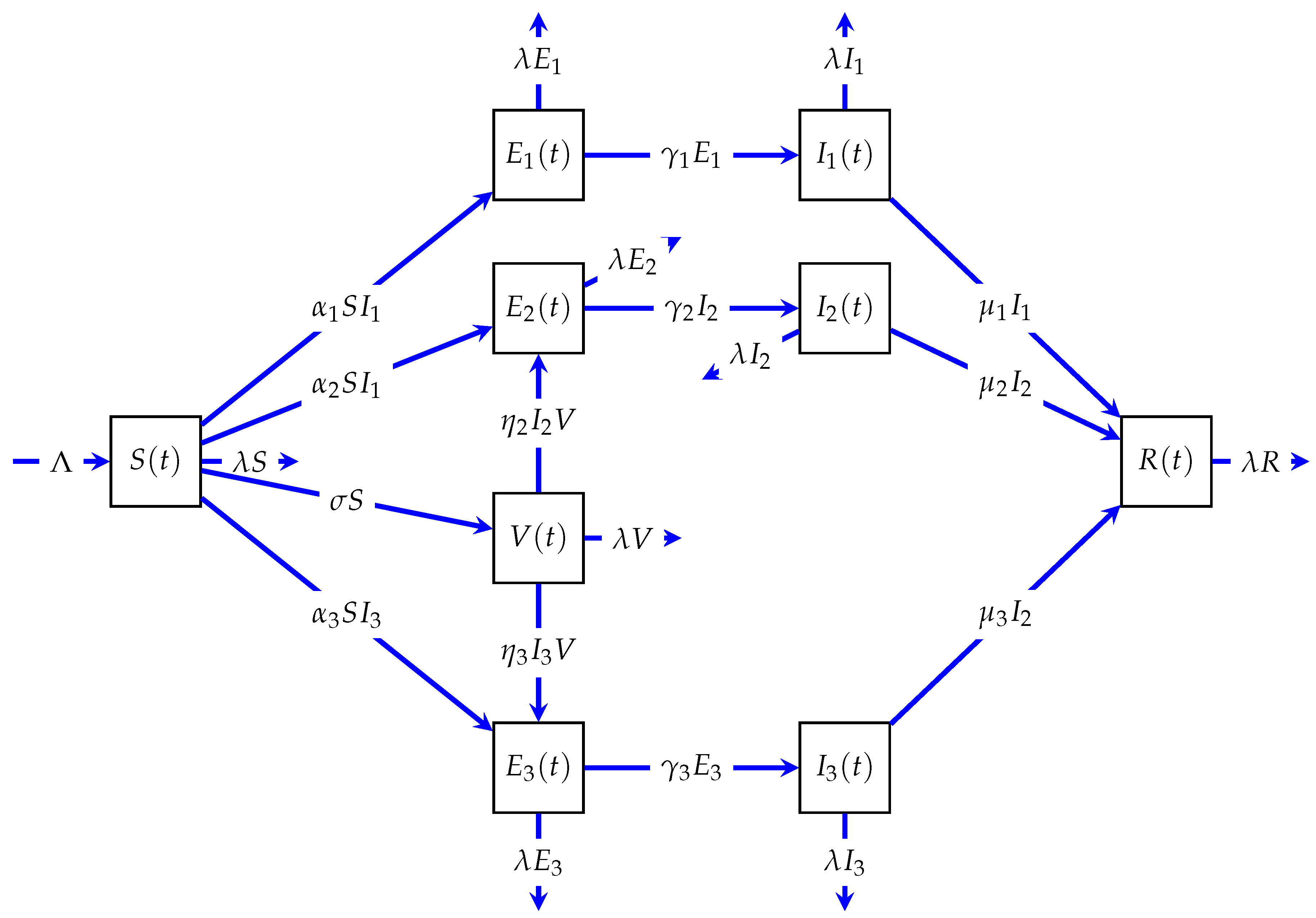
In the above, , and R represent, respectively, the compartment of susceptible individuals, vaccinated individuals, strain-1-exposed individuals, stain-2-exposed individuals, stain-3-exposed individuals, strain-1-infected individuals, stain-2-infected individuals, stain-3-infected individuals, and recovered individuals. The parameters of this model (1) are given in Table 1, and the description of all model (1) elements is represented in Figure 1. We assume that there is no reinfection of recovered individuals.
This work is divided as follows: In Section 2, we give some results of the existence, positivity, and boundedness of model (1) solutions. In Section 3, we prove the global stability of equilibrium points. Numerical simulations are presented in Section 4 to validate the different results found in the theoretical part. The last section concludes this work.
2. Existence, Positivity, and Boundedness of Solutions
In this section, we prove that model (1) has a unique, non-negative, and bounded solution for all .
Proposition 1.
For any non-negative initial condition, model (1) has a unique solution. In addition, this solution remains non-negative and bounded for all .
Proof.
First, we prove that system (1) has a unique solution. We can reformulate the model (1) as follows:
with
and
We remark that F is a Lipschitz function; moreover, we have
with
and
Thus, model (1) has a unique solution in .
Now, we prove that this solution remains non-negative.
Thus, this solution remains non-negative for all .
Finally, for the boundedness of this solution, we verify that the biologically feasible region
is positively invariant.
Let the total population
Then, we conclude that P is positively invariant. Therefore, we can conclude that model (1) has a unique, positive, and bounded solution . □
3. Analysis of the Model
In this section, we prove that there exists a disease-free equilibrium point and four equilibrium points. The global stability of these equilibrium points using the Lyapunov functional method is proved. As the first eight equations of system (1) are independent of the ninth equation, and also the total number of population N is determined using Equation (15), system (1) can be reduced to the following system:
with
3.1. The Basic Reproduction Number Calculation
The basic reproduction number is the number of secondary infection cases caused by one infected individual in a population constituted only by susceptible individuals, and mathematically, the basic reproduction number is the spectral radius of the matrix called the next-generation matrix , with F as the positive matrix of new infection cases and V as the matrix of the transition of the infections.
Let
and
Thus, we have
3.2. Steady States
Model (14) has one disease-free equilibrium point, and the other four endemic equilibrium points are given by
- The disease-free equilibrium , where
- The strain-1 endemic equilibrium , where
- The strain-2 endemic equilibrium , wherewhere is solution of the equation with .
- The strain-3 endemic equilibrium , wherewhere is solution of the equation with .
- The total strain endemic equilibrium , wherewhere and are the roots of the following equations:andwhere
Remark 1.
From the components of the equilibrium points, we conclude that points exist when, and.
3.3. Global Stability
In this section, we give the different theorems concerning the global stability of the different equilibrium points:
Theorem 1.
If , and , then the disease-free equilibrium is globally asymptotically stable.
Proof.
We consider the following Lyapunov function in :
The time derivative of is given by
As and , we will have
Thus, when and , we will have . Thus, the disease-free equilibrium point is globally asymptotically stable. □
Theorem 2.
If , and , then the strain-1 endemic equilibrium point is globally asymptotically stable.
Proof.
We consider the following Lyapunov function in :
The time derivative of is given by
As is an equilibrium point of system (14), we will have
Thus, after some simplifications and factorizations, we will have
As the arithmetic mean is greater than or equal to the geometric mean, we will have
and
Moreover,
Then, when and , we will have . Thus, the strain-1 endemic equilibrium point is globally asymptotically stable. □
For the global stability of the equilibrium point , we assume that this point verifies the following condition:
Theorem 3.
If , and , then the strain-2 endemic equilibrium point is globally asymptotically stable.
Proof.
We consider the following Lyapunov function in :
The time derivative of is given by
As is an equilibrium point of system (14), we will have
Thus, after some simplifications and factorizations, we will have
As the arithmetic mean is greater than or equal to the geometric mean, we will have
and
As verifies condition , when and , we will have . Thus, the strain-2 endemic equilibrium point is globally asymptotically stable. □
For the global stability of the equilibrium point , we assume that this point verifies the following condition:
Theorem 4.
If and , then the strain-3 endemic equilibrium point is globally asymptotically stable.
Proof.
We consider the following Lyapunov function in :
The time derivative of is given by
As is an equilibrium point of system (14), we will have
Thus, after some simplifications and factorizations, we will have
As the arithmetic mean is greater than or equal to the geometric mean, we will have
and
As verifies condition , when and , we will have . Thus, the strain-3 endemic equilibrium is globally asymptotically stable. □
Theorem 5.
If , then the total endemic equilibrium point is globally asymptotically stable.
Proof.
We consider the following Lyapunov function in :
The time derivative of is given by
As is an equilibrium point of system (14), we will have
Thus, after some simplifications and factorizations, we will have
As the arithmetic mean is greater than or equal to the geometric mean, we will have
and
Moreover, if and , we will have
and
Then, when , we will have .Thus, the total endemic equilibrium is globally asymptotically stable. □
4. Numerical Simulations
In order to confirm our theoretical results, some numerical simulations and discussions are presented in this section by using the value of the parameter given in Table 2. We performed our numerical simulations with the Runge–Kutta method [44] to test the effect of the vaccine in reducing the infection; in reality, the vaccination against a strain of an infectious disease such as COVID-19 leads to a reduction in the total number of infections.
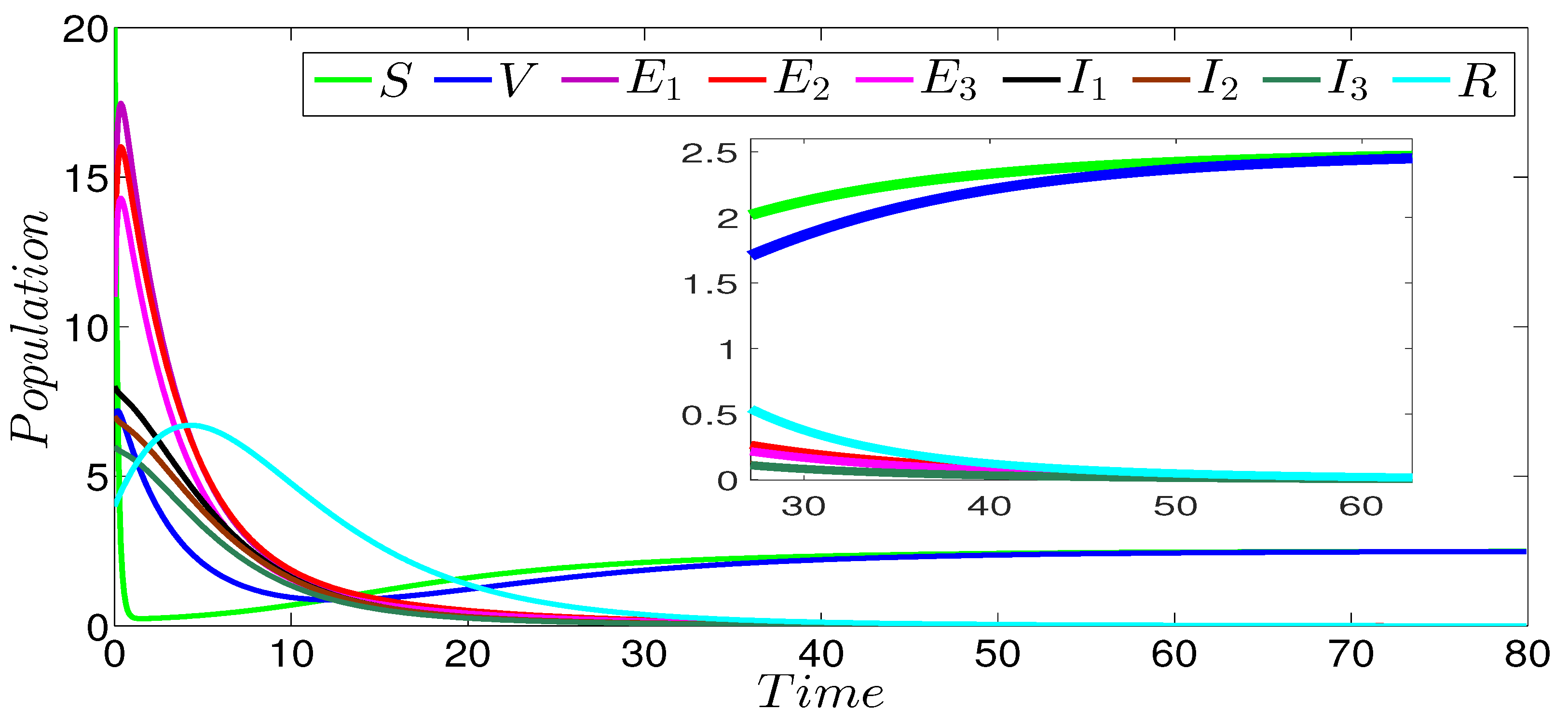
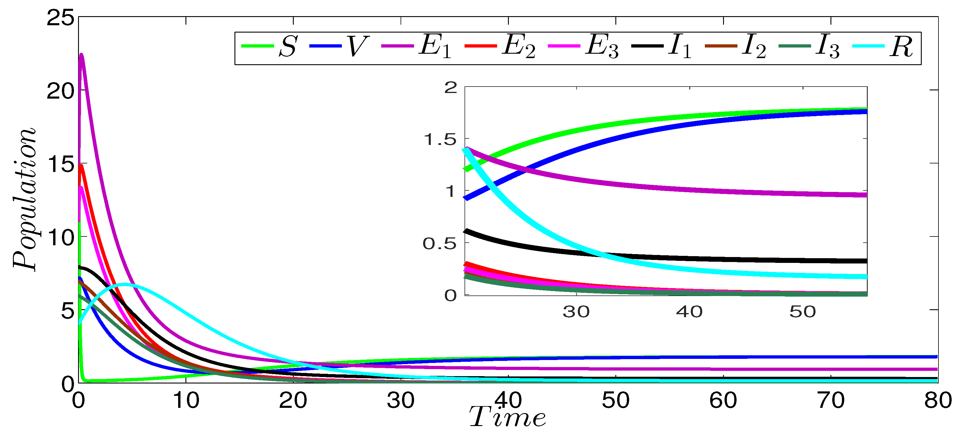
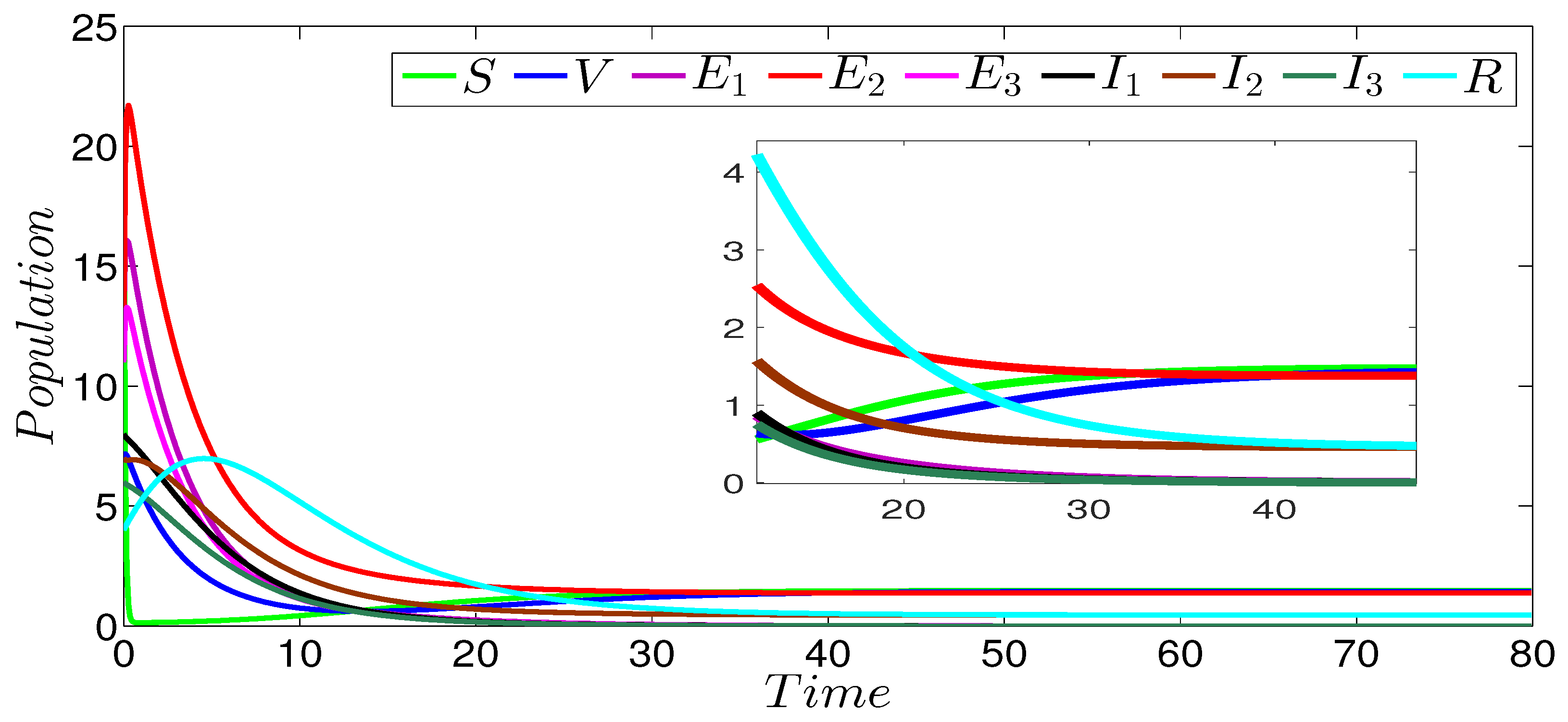
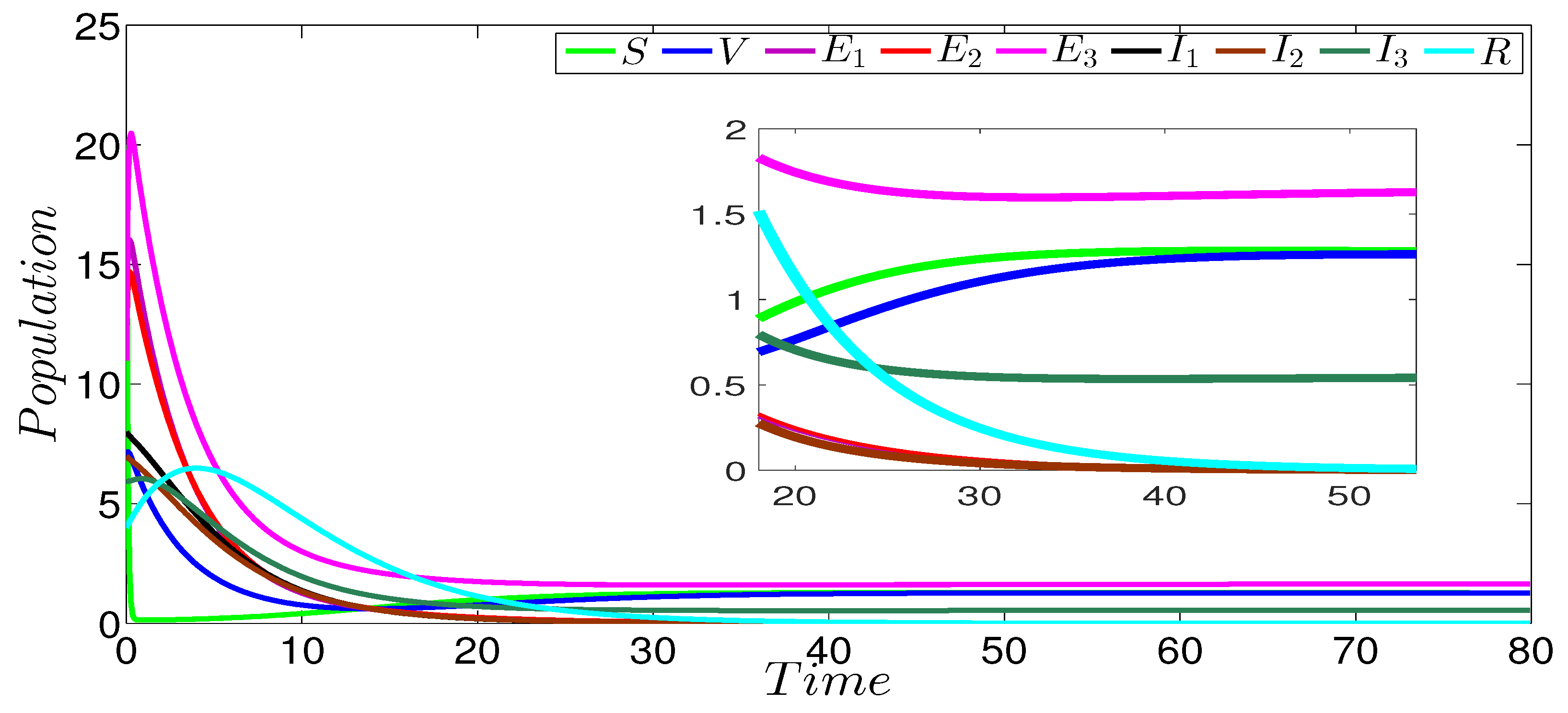
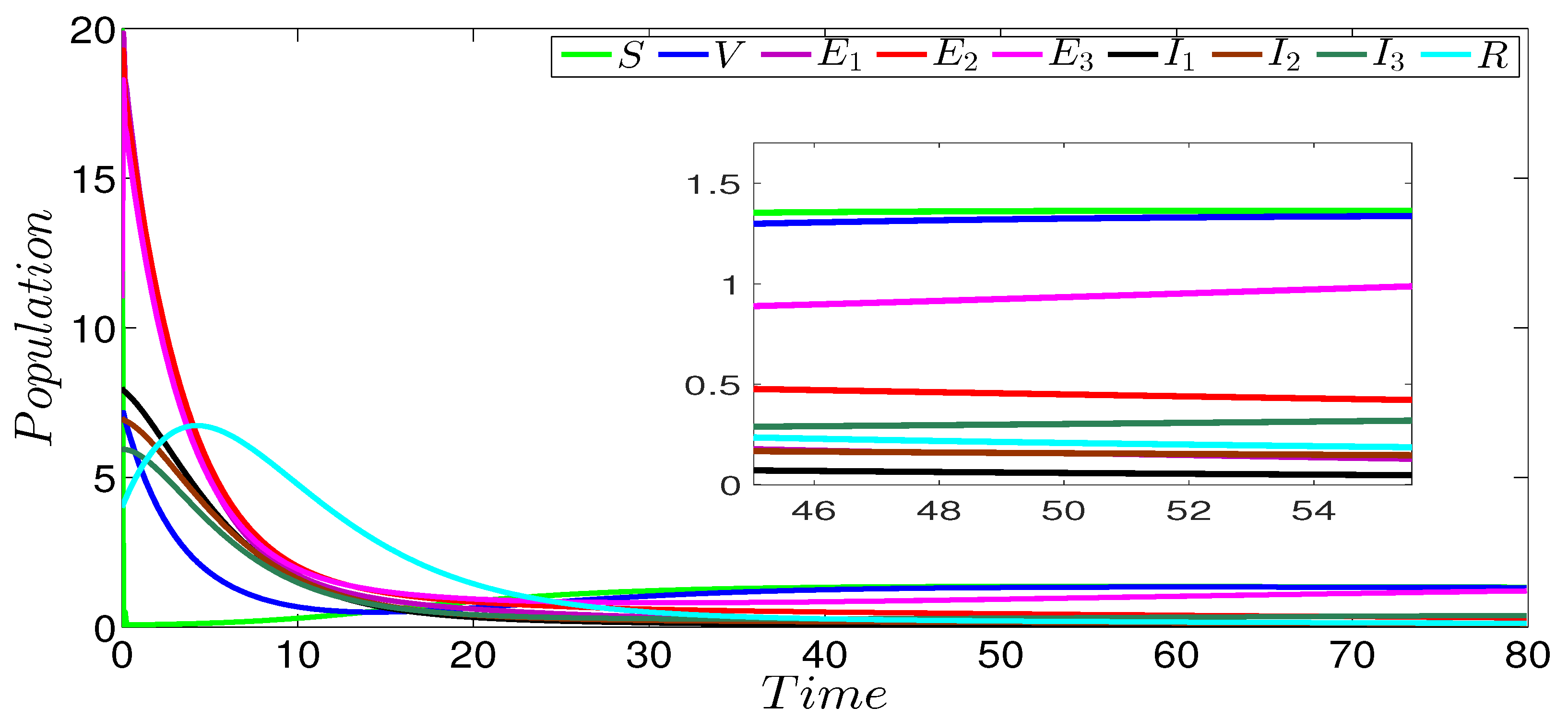
Figure 2 shows the dynamics of the infection of the three strains SVEIR model. In this figure, we can see that the curves drop to zero, except the curves representing the susceptible and vaccinated individuals. This behavior is clearly observed in the zoomed part of the same figure. The obtained numerical result perfectly coincides with our theoretical result given in Theorem 1 concerning the global stability of the disease-free equilibrium ( and ). Figure 3 describes the evolution of the different three strains of model components. In this figure, we notice that the first strain persists in contrast to the others strains that die out. The zoomed part of the same figure more clearly shows the persistence of the first strain. The strain-1 basic reproduction number is greater than 1 (), and the basic reproduction numbers of the other strains are less than 1 (). This numerical result verifies our theoretical result given in Theorem 2 concerning the global stability of the strain-1 endemic equilibrium. Figure 4 shows the global stability of the strain-2 endemic equilibrium, it is easy to observe that strain-2 persists while the other strains die out. The zoomed part of the same figure more clearly shows the persistence of the second strain. The basic reproduction number of this strain is greater than 1 (), while the basic reproduction numbers of the other strains are less than 1 (), which confirms our theoretical result given in Theorem 3 concerning the global stability of the strain-2 endemic equilibrium. Figure 5 describes the global stability of the strain-3 endemic equilibrium. This figure shows that strain-3 persists, while the other strains die out. The zoomed part of the same figure more clearly shows the persistence of the third strain. The basic reproduction number of this strain is greater than 1 (), while the basic reproduction numbers of the other strains are less than 1 (, ), which confirms our theoretical result given in Theorem 4 concerning the global stability of this equilibrium point. For the case of the global stability of the total endemic equilibrium, Figure 6 shows that all the strains persist. The zoomed part of the same figure more clearly shows the persistence of the all acting strains. Indeed, the basic reproduction number of every strain is greater than 1 ( and ); this numerical result is in a good argument with our theoretical result given in Theorem 5 concerning the global stability of this equilibrium point.
5. Conclusions
In this paper, we analyzed a three-strain epidemic model with a vaccination strategy. The model contains nine compartments, namely susceptible individuals, vaccinated individuals, the three categories of exposed individuals, the three categories of infected individuals, and the recovered individuals. We started the analysis of this model by giving the different results of the existence, positivity, and boundedness of the model solutions. The suggested model has five steady states, namely the disease-free equilibrium, the strain-1 endemic equilibrium, the strain-2 endemic equilibrium, the strain-3 endemic equilibrium, and the total endemic equilibrium. By using the new generation method, we obtained the three basic reproduction numbers , and . Next, by using some suitable Lyapunov functions, we gave the global stability of the different steady states. This stability depends on different values of basic reproduction numbers. More precisely, if the three basic reproduction numbers are less than 1, the free equilibrium point is globally asymptotically stable. In addition, if , and , the strain-1 endemic equilibrium point is globally asymptotically stable, while the strain-2 endemic equilibrium point and strain-3 endemic equilibrium point are, respectively, globally asymptotically stable if , and ; and , and . Finally, the total endemic equilibrium is globally asymptotically stable if all reproduction numbers are greater than 1. We showed that any strain with a higher reproduction number value outperforms the other strains. Numerical simulations were given in order to confirm and validate our theoretical results. It was observed that, in order to eradicate an infection, the basic reproduction numbers of all the strains must be less than unity.
Author Contributions
Writing—original draft, Z.Y.; Writing—review & editing, Z.Y. and K.A.; Visualization, K.A.; Supervision, K.A. All authors have read and agreed to the published version of the manuscript.
Funding
This research received no external funding.
Conflicts of Interest
The authors declare no conflict of interest.
References
- Arruda, E.F.; Das, S.S.; Dias, C.M.; Pastore, D.H. Modelling and optimal control of multi strain epidemics, with application to COVID-19. PLoS ONE 2021, 16, e0257512. [Google Scholar] [CrossRef] [PubMed]
- Khyar, O.; Allali, K. Global dynamics of a multi-strain SEIR epidemic model with general incidence rates: Application to COVID-19 pandemic. Nonlinear Dyn. 2020, 102, 489–509. [Google Scholar] [CrossRef] [PubMed]
- Chen, W.; Tuerxun, N.; Teng, Z. The global dynamics in a wild-type and drug-resistant HIV infection model with saturated incidence. Adv. Differ. Equ. 2020, 2020, 1–16. [Google Scholar] [CrossRef] [Green Version]
- Amine, S.; Allali, K. Dynamics of a time-delayed two-strain epidemic model with general incidence rates. Chaos Solitons Fractals 2021, 153, 111527. [Google Scholar]
- Sweilam, N.H.; AL–Mekhlafi, S.M. Optimal control for a time delay multi-strain tuberculosis fractional model: A numerical approach. IMA J. Math. Control. Inf. 2019, 36, 317–340. [Google Scholar] [CrossRef]
- Kermack, W.O.; McKendrick, A.G. A contribution to the mathematical theory of epidemics. Proc. R. Soc. Lond. Ser. A 1927, 115, 700–721. [Google Scholar]
- Godio, A.; Pace, F.; Vergnano, A. SEIR modeling of the Italian epidemic of SARS-CoV-2 using computational swarm intelligence. Int. J. Environ. Res. Public Health 2020, 17, 3535. [Google Scholar] [CrossRef] [PubMed]
- Rangasamy, M.; Chesneau, C.; Martin-Barreiro, C.; Leiva, V. On a novel dynamics of SEIR epidemic models with a potential application to COVID-19. Symmetry 2022, 14, 1436. [Google Scholar] [CrossRef]
- Marinca, B.; Marinca, V.; Bogdan, C. Dynamics of SEIR epidemic model by optimal auxiliary functions method. Chaos Solitons Fractals 2021, 147, 110949. [Google Scholar] [CrossRef]
- Bajiya, V.P.; Tripathi, J.P.; Kakkar, V.; Wang, J.; Sun, G. Global dynamics of a multi-group SEIR epidemic model with infection age. Chin. Ann. Math. Ser. B 2021, 42, 833–860. [Google Scholar] [CrossRef]
- Paul, S.; Mahata, A.; Ghosh, U.; Roy, B. Study of SEIR epidemic model and scenario analysis of COVID-19 pandemic. Ecol. Genet. Genom. 2021, 19, 100087. [Google Scholar] [CrossRef] [PubMed]
- Weinstein, S.J.; Holl, M.S.; Rogers, K.E.; Barlow, N.S. Analytic solution of the SEIR epidemic model via asymptotic approximant. Phys. D Nonlinear Phenom. 2020, 411, 132633. [Google Scholar] [CrossRef] [PubMed]
- Upadhyay, R.K.; Pal, A.K.; Kumari, S.; Roy, P. Dynamics of an SEIR epidemic model with nonlinear incidence and treatment rates. Nonlinear Dyn. 2019, 96, 2351–2368. [Google Scholar] [CrossRef]
- Qiu, X.; Nergiz, A.I.; Maraolo, A.E.; Bogoch, I.I.; Low, N.; Cevik, M. The role of asymptomatic and presymptomatic infection in SARS-CoV-2 transmission—A living systematic review. Clin. Microbiol. Infect. 2021, 27, 511–519. [Google Scholar] [CrossRef] [PubMed]
- Wang, J.J.; Zhang, J.Z.; Jin, Z. Analysis of an SIR model with bilinear incidence rate. Nonlinear Anal. Real World Appl. 2010, 11, 2390–2402. [Google Scholar] [CrossRef]
- Junhua, C.; Shengjun, W. Modeling and analyzing the spread of worms with bilinear incidence rate. In Proceedings of the 2009 Fifth International Conference on Information Assurance and Security, Xi’an, China, 18–20 August 2009; IEEE: Piscataway, NJ, USA, 2009; Volume 2, pp. 167–170. [Google Scholar]
- Roy, M.; Pascual, M. On representing network heterogeneities in the incidence rate of simple epidemic models. Ecol. Complex. 2006, 3, 80–90. [Google Scholar] [CrossRef]
- Li, J.H.; Cui, N.; Niu, L.; Zhang, J. Dynamic analysis of an SEIS model with bilinear incidence rate. In Proceedings of the 2011 International Conference on Computer Science and Network Technology, Harbin, China, 24–26 December 2011; IEEE: Piscataway, NJ, USA, 2011; Volume 4, pp. 2268–2271. [Google Scholar]
- Liu, S.; Zhang, L.; Zhang, X.B.; Li, A. Dynamics of a stochastic heroin epidemic model with bilinear incidence and varying population size. Int. J. Biomath. 2019, 12, 1950005. [Google Scholar] [CrossRef]
- Kuddus, M.A.; McBryde, E.S.; Adekunle, A.I.; Meehan, M.T. Analysis and simulation of a two-strain disease model with nonlinear incidence. Chaos Solitons Fractals 2022, 155, 111637. [Google Scholar] [CrossRef]
- Meehan, M.T.; Cocks, D.G.; Trauer, J.M.; McBryde, E.S. Coupled, multi-strain epidemic models of mutating pathogens. Math. Biosci. 2018, 296, 82–92. [Google Scholar] [CrossRef] [Green Version]
- Sardar, T.; Ghosh, I.; Rodó, X.; Chattopadhyay, J. A realistic two-strain model for MERS-CoV infection uncovers the high risk for epidemic propagation. PLoS Neglected Trop. Dis. 2020, 14, e0008065. [Google Scholar] [CrossRef]
- Khatua, A.; Pal, D.; Kar, T.K. Global Dynamics of a Diffusive Two-Strain Epidemic Model with Non-Monotone Incidence Rate. Iran. J. Sci. Technol. Trans. A Sci. 2022, 46, 859–868. [Google Scholar] [CrossRef]
- Bentaleb, D.; Amine, S. Lyapunov function and global stability for a two-strain SEIR model with bilinear and non-monotone incidence. Int. J. Biomath. 2019, 12, 1950021. [Google Scholar] [CrossRef]
- Meskaf, A.; Khyar, O.; Danane, J.; Allali, K. Global stability analysis of a two-strain epidemic model with non-monotone incidence rates. Chaos Solitons Fractals 2020, 133, 109647. [Google Scholar] [CrossRef]
- Yaagoub, Z.; Danane, J.; Allali, K. Global Stability Analysis of Two-Strain SEIR Epidemic Model with Quarantine Strategy. In Nonlinear Dynamics and Complexity; Springer: Cham, Switzerland, 2022; pp. 469–493. [Google Scholar]
- El-Shabasy, R.M.; Nayel, M.A.; Taher, M.M.; Abdelmonem, R.; Shoueir, K.R. Three wave changes, new variant strains, and vaccination effect against COVID-19 pandemic. Int. J. Biol. Macromol. 2022, 204, 161–168. [Google Scholar] [CrossRef] [PubMed]
- De León, U.A.P.; Avila-Vales, E.; Huang, K.L. Modeling COVID-19 dynamic using a two-strain model with vaccination. Chaos Solitons Fractals 2022, 157, 111927. [Google Scholar] [CrossRef] [PubMed]
- Tchoumi, S.Y.; Rwezaura, H.; Tchuenche, J.M. Dynamic of a two-strain COVID-19 model with vaccination. Results Phys. 2022, 39, 105777. [Google Scholar] [CrossRef] [PubMed]
- Guo, J.; Wang, S.M. Threshold dynamics of a time-periodic two-strain SIRS epidemic model with distributed delay. AIMS Math. 2022, 7, 6331–6355. [Google Scholar] [CrossRef]
- Chang, Y.C.; Liu, C.T. A Stochastic Multi-Strain SIR Model with Two-Dose Vaccination Rate. Mathematics 2022, 10, 1804. [Google Scholar] [CrossRef]
- Angeli, M.; Neofotistos, G.; Mattheakis, M.; Kaxiras, E. Modeling the effect of the vaccination campaign on the COVID-19 pandemic. Chaos Solitons Fractals 2022, 154, 111621. [Google Scholar] [CrossRef] [PubMed]
- Marinov, T.T.; Marinova, R.S. Adaptive SIR model with vaccination: Simultaneous identification of rates and functions illustrated with COVID-19. Sci. Rep. 2022, 12, 1–13. [Google Scholar] [CrossRef]
- Lin, L.; Zhao, Y.; Chen, B.; He, D. Multiple COVID-19 waves and vaccination effectiveness in the united states. Int. J. Environ. Res. Public Health 2022, 19, 2282. [Google Scholar] [CrossRef]
- Kayanja, A.; Abola, B.; Kikawa, C.; Oyo, B.; Ssematimba, A. Modelling the transmission dynamics of a multi-strain SARS-CoV-2 epidemic with vaccination for an emerging strain. Res. Sq. 2022. [Google Scholar] [CrossRef]
- Bugalia, S.; Tripathi, J.P.; Wang, H. Mutations make pandemics worse or better: Modeling SARS-CoV-2 variants and imperfect vaccination. arXiv 2022, arXiv:2201.06285. [Google Scholar]
- El Hajji, M.; Albargi, A.H. A mathematical investigation of an “SVEIR” epidemic model for the measles transmission. Math. Biosc. Eng. 2022, 19, 2853–2875. [Google Scholar] [CrossRef] [PubMed]
- Shoaib, M.; Anwar, N.; Ahmad, I.; Naz, S.; Kiani, A.K.; Raja, M.A.Z. Intelligent networks knacks for numerical treatment of nonlinear multi-delays SVEIR epidemic systems with vaccination. Int. J. Mod. Phys. B 2022, 36, 2250100. [Google Scholar] [CrossRef]
- Xu, J. Global dynamics for an SVEIR epidemic model with diffusion and nonlinear incidence rate. Bound. Value Probl. 2022, 2022, 1–13. [Google Scholar] [CrossRef]
- Nasution, H.; Khairani, N.; Ahyaningsih, F.; Alamsyah, F. Mathematical modeling of the spread of corona virus disease 19 (COVID-19) with vaccines. AIP Conf. Proc. 2022, 2659, 110009. [Google Scholar]
- Sun, D.; Li, Y.; Teng, Z.; Zhang, T.; Lu, J. Dynamical properties in an SVEIR epidemic model with age-dependent vaccination, latency, infection, and relapse. Math. Methods Appl. Sci. 2021, 44, 12810–12834. [Google Scholar] [CrossRef]
- Onwubuya, I.O.; Madubueze, C.E. SVEIR model of an infectious disease among infected immigrants with nonlinear incidence rate. J. Niger. Soc. Math. Biol. 2021, 4, 1–18. [Google Scholar]
- Baba, I.A.; Kaymakamzade, B.; Hincal, E. Two-strain epidemic model with two vaccinations. Chaos Solitons Fractals 2018, 106, 342–348. [Google Scholar] [CrossRef]
- Macías-Díaz, J.E.; Raza, A.; Ahmed, N.; Rafiq, M. Analysis of a nonstandard computer method to simulate a nonlinear stochastic epidemiological model of coronavirus-like diseases. Comput. Methods Programs Biomed. 2021, 204, 106054. [Google Scholar] [CrossRef]
Figure 1.
The diagram of three-strain model.

Figure 2.
Stability of disease-free equilibrium of the three-strain SVEIR model with = 0.55, = 0.82, and .
Figure 2.
Stability of disease-free equilibrium of the three-strain SVEIR model with = 0.55, = 0.82, and .

Figure 3.
Stability of the strain-1 endemic equilibrium of the three-strain SVEIR model with and .

Figure 4.
Stability of the strain-2 endemic equilibrium of the three-strain SVEIR model with , and .
Figure 4.
Stability of the strain-2 endemic equilibrium of the three-strain SVEIR model with , and .

Figure 5.
Stability of the strain-3 endemic equilibrium of three-strain SVEIR model with = 0.55, = 0.82, and .
Figure 5.
Stability of the strain-3 endemic equilibrium of three-strain SVEIR model with = 0.55, = 0.82, and .

Figure 6.
Stability the total endemic equilibrium of the three-strain SVEIR model with = 1.38, = 1.93, and .
Figure 6.
Stability the total endemic equilibrium of the three-strain SVEIR model with = 1.38, = 1.93, and .


Table 1.
Description of the parameters in the model.
| Parameters | Description |
|---|---|
| The recruitment rate of the population | |
| The natural mortality rate | |
| The infection rate of strain-1 | |
| The infection rate of strain-2 | |
| The infection rate of strain-3 | |
| The vaccination rate of the strain-1 individuals | |
| The transmission rate of vaccinated individuals to strain-2 | |
| The transmission rate of vaccinated individuals to strain-3 | |
| The average latency period of the strain-1 | |
| The average latency period of the strain-2 | |
| The average latency period of the strain-3 | |
| The average infection period of the strain-1 | |
| The average infection period of the strain-2 | |
| The average infection period of the strain-3 |
Table 2.
The parameter values of system (1).
Disclaimer/Publisher’s Note: The statements, opinions and data contained in all publications are solely those of the individual author(s) and contributor(s) and not of MDPI and/or the editor(s). MDPI and/or the editor(s) disclaim responsibility for any injury to people or property resulting from any ideas, methods, instructions or products referred to in the content. |
© 2023 by the authors. Licensee MDPI, Basel, Switzerland. This article is an open access article distributed under the terms and conditions of the Creative Commons Attribution (CC BY) license (https://creativecommons.org/licenses/by/4.0/).
Share and Cite
MDPI and ACS Style
Yaagoub, Z.; Allali, K. Global Stability of Multi-Strain SEIR Epidemic Model with Vaccination Strategy. Math. Comput. Appl. 2023, 28, 9. https://doi.org/10.3390/mca28010009
AMA Style
Yaagoub Z, Allali K. Global Stability of Multi-Strain SEIR Epidemic Model with Vaccination Strategy. Mathematical and Computational Applications. 2023; 28(1):9. https://doi.org/10.3390/mca28010009
Chicago/Turabian StyleYaagoub, Zakaria, and Karam Allali. 2023. "Global Stability of Multi-Strain SEIR Epidemic Model with Vaccination Strategy" Mathematical and Computational Applications 28, no. 1: 9. https://doi.org/10.3390/mca28010009