

Temperature Patterns in TSA for Different Frequencies and Material Properties: A FEM Approach

1
Faculty of Engineering, University of Porto, Rua Dr. Roberto Frias, s/n, 4200-465 Porto, Portugal
2
Institute of Science and Innovation in Mechanical and Industrial Engineering (INEGI), Rua Dr. Roberto Frias, Campus da FEUP, 400, 4200-465 Porto, Portugal
*
Author to whom correspondence should be addressed.
Math. Comput. Appl. 2023, 28(1), 8; https://doi.org/10.3390/mca28010008
Submission received: 17 October 2022
/
Revised: 26 December 2022
/
Accepted: 29 December 2022
/
Published: 6 January 2023
(This article belongs to the Special Issue Mathematical and Computational Modelling in Mechanics of Materials and Structures)
Abstract
:Thermography techniques are gaining popularity in structural integrity monitoring and analysis of mechanical systems’ behavior because they are contactless, non-intrusive, rapidly deployable, applicable to structures under harsh environments, and can be performed on-site. More so, the use of image optical techniques has grown quickly over the past several decades due to the progress in the digital camera, infrared camera, and computational power. This work focuses on thermoelastic stress analysis (TSA), and its main goal was to create a computational model based on the finite element method that simulates this technique, to evaluate and quantify how the changes in material properties, including orthotropic, affect the results of the stresses obtained with TSA. The numeric simulations were performed for two samples, compact and single lap joints. when comparing the numeric model developed with previous laboratory tests, the results showed a good representation of the stress test for both samples. The created model is applicable to various materials, including fiber-reinforced composites. This work also highlights the need to perform laboratory tests using anisotropic materials to better understand the TSA potential and improve the developed models.
Keywords:
TSA; mechanical stress; FEM; transient; material properties; orthotropic; composites; thermal conductivity1. Introduction
Structural integrity monitoring is a vital process of any mechanical system that analyzes its behavior in order to detect defects and prevent malfunctions and failures. With the major importance of structural integrity, there is interest in studying new and unconventional techniques with new characteristics and advantages. Thermography techniques are gaining popularity because they are contactless, real-time, non-intrusive, and can be performed on-site. The range of applications of these techniques is vast, going beyond structural integrity monitoring into failure detection, fatigue assessment, and residual stress measurement. There are some works that focus on fatigue assessment, determining fatigue limit, fatigue strength evaluation, damage location, and life prediction, showing the potential and advantages of thermography techniques [1,2,3]. The usage of thermography has also been employed to characterize material properties that are not directly measurable [4,5,6,7]. These measures can be used to obtain properties for numeric simulations or directly used in research or industrial applications. The use of image techniques has grown quickly over the past several decades due to the progress in the digital camera, infrared camera, and computational power [8,9]. Using image (or field) nature techniques enables the identification of strain concentrations and damage more accurately. This could be done for identifying the presence of defects or to quantify them. These analyses are more likely to be performed for high value and high-cost components, such as carbon-fiber-reinforced polymer (CFRP) [10,11]. One of the most interesting techniques in this field is thermoelastic stress analysis (TSA) [12,13,14,15,16].
TSA fundamentals are based on the thermoelastic effect, in which small temperature changes are induced in a solid component when a cyclic load is applied. The results of TSA depend on various parameters, including the load type (sinusoidal, square-wave, triangular, etc.), its amplitude/average, specimen mean temperature, and material type (isotropic, orthotropic or anisotropic). If adiabatic and reversible conditions are achieved, these temperature changes are proportional to the sum of the principal stresses. These temperature variations, which are in the order of tens of mK in metallic materials, can be measured at the surface of a component using infrared detectors. Therefore, by measuring the variations in temperature due to the applied cyclic load, the first stress invariant can be determined from the detector’s output. The stress fields obtained with computational modeling and the finite element method (FEM) are often used in comparisons, and the results obtained normally show a satisfying agreement [13,16,17,18,19,20].
Besides the typical applications of this technique, such as fatigue failure and crack analysis, a point of focus of TSA applications is their expansion to materials that are not isotropic, including composites, for example, which are of great interest to the engineering industry. Orthotropic materials have different property values in different directions, contrary to isotropic materials. This means that the considerations made in the classic thermoelastic theory are not applicable and the equations for these cases are different; the measured temperature variations are proportional to a linear combination of the principal stresses instead. The thermoelastic coefficient values change with direction also beacuse the coefficient of thermal expansion also varies. Besides this, the effects of the change on some thermal properties on the obtained stresses, such as the conductivity, are quite unclear. Regarding composite materials, TSA is more complicated, since the stresses depend on the constitutive material properties and the ply stacking sequence as well as the fiber orientation. Heat flux with the surroundings is usually negligible, but between plies of a laminate can be sufficient to negate the simpler thermoelasticity process of only measuring the surface stresses. Furthermore, the internal heat transfer effects can depend on the loading frequency. This influences the thermal patterns measured by TSA, in particular, in areas with great stress variation gradients. The TSA theory presented by William N.S. Jr. does not consider the influence of the stimulation frequency [12]. However, this has great influence in the TSA results [14] TSA allows one to analyze delamination failure in composites, the most common failure type in these materials. Estimation of the delamination crack length and crack growth can be carried out [21,22,23]. TSA can also evaluate fiber breakage and matrix cracking [24].
The relation between the thermoelastic theory and the material type is complex, and many studies focus on it. The main goal of this works was to take in account various effects that influence the obtained results, such as the mean stress at a crack tip, residual stresses, and non-isotropy. To take in account these effects, the authors propose new TSA models and equations that allow materials to undergo any loading conditions and orthotropic/anisotropic conditions too [25,26,27,28,29].
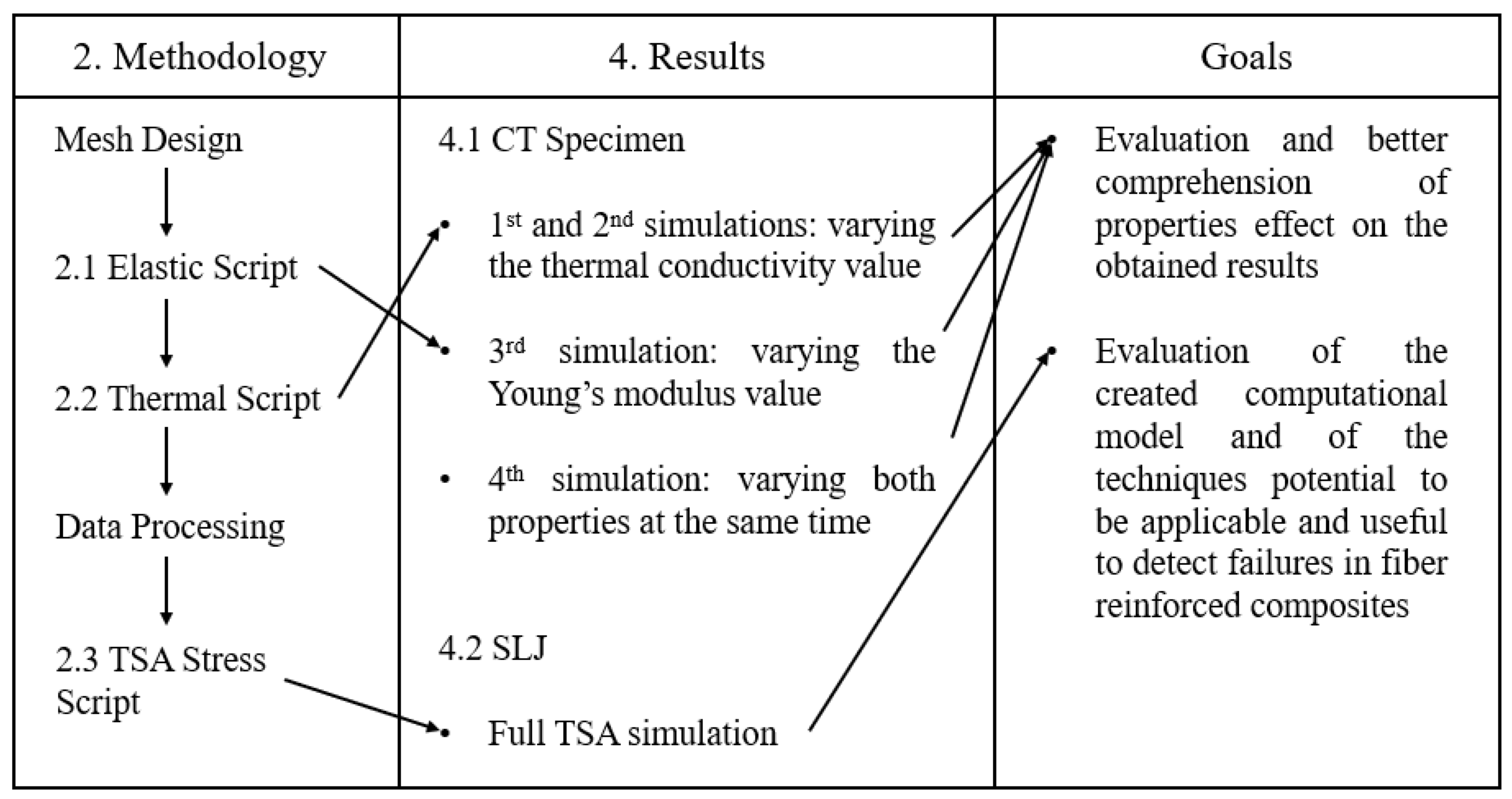
The goal for this work was to create a finite element-based computational model that simulates a material’s properties’ influences on TSA (including the frequency influence) that is applicable to orthotropic materials, including composites. The created model was tested in order to evaluate and quantify how the changes in material properties and load frequency affect the results of the obtained stresses with TSA. To have a better comprehension of this work’s goals and planifications, a workflow was designed, as shown in Figure 1. Throughout this document, the methodology of the model is presented first, followed by the procedure and results. The last part is reserved to results discussion and conclusions.
2. Methodology
This section describes the methodology used to create a computational model that simulates the TSA technique. A model was created using MATLAB software using the finite element method (FEM). The model and its approximations had a major influence on the results that are described by Erik G. Thompson in [30]. TSA relates the principal stresses’ sum and the temperature changes in a body due to the application of a cyclic load. Thus, the first step towards this goal is to perform a static elastic simulation to obtain a stress-sum distribution resulting from the application of a static load with a value equal to the amplitude value of the desired cyclic load. Next, the obtained results from this simulation are transformed into an external heat source to transpose the results to the next stage, a thermal simulation. Finally, with this information, and after data processing with the help of a fast Fourier transform (FFT), the signal amplitude is extracted, and the TSA equations can be applied. Then, a full-field stress-sum distribution map is obtained.
2.1. Elastic Simulation
Consider plane elasticity and its governing equation, Equation (1), where K is the global stiffness matrix, {u} is the unknown displacement’s vector, and {F} is the global external load vector. Then, Equation (1) can be applied to each element and then assembled to represent the entire domain [31].
The balance between size and accuracy was found considering only 2D analysis, more specifically in a plane-stress state. In the simulations, 4-node elements were used to balance the mesh detailing and computational cost [31]. The stiffness matrix for each element was calculated using Equation (2), where B, D, and J represent the strain, elasticity, and Jacobian matrices, and the following considerations were made:
- Usage of isoparametric elements, because it is suitable for numerical quadrature and systematic definition of the interpolation functions. This means a change from x and y coordinates to and , with the relationship between both being a matrix of interpolation functions, N. The interpolation function is relative to node i, and its value is one at that node and null in the finite elements that do not share this node;
- Application of numerical quadrature, where the obtained integral for the calculation of K according to the FEM can be replaced by a summation of the integrated function applied at several Gauss points, (with (, ) coordinates), multiplied by the respective weight, . The number of Gauss points chosen was four, meaning full integration (instead of 1 GP, reduced integration) because shear locking is not a problem in this study, and to prevent the hourglass effect [31].
The Jacobian matrix is obtained by multiplying a matrix of the interpolation functions’ partial derivatives of each node x and y coordinates. The strain matrix is obtained by multiplying the inverse of the Jacobian matrix by the same partial derivative matrix used before.
Since a plane stress state is being considered, and orthotropic materials, the elasticity matrix is given by Equation (3), where represents the Young’s modulus and the Poisson’s coefficient in i and j directions. The shear modulus, , is given by Equation (4) [32,33].
The external loading vector was calculated by applying Equation (5). As one can see, both external forces applied over the element area and surface traction, respectively, b and , take part in this relation. Included in the boundary conditions are also restricted movements, which can be applied in the global stiffness matrix by multiplying the value by , in the corresponding restricted nodal direction, originating an overly excessive stiffness and preventing movement in that direction. With both K and {F} calculated, the nodal displacements are obtained with the use of Equation (1). With these values known, both deformations and stress vectors can be easily calculated by applying Equation (6).
2.2. Thermal Simulation
With the FEM approximations, the problem comes in the form of Equation (7), where C is the mass matrix, {} is the temperature with respect to time, {} is the temperature’s time derivative, and {Q} is the external heat vector. This analysis is divided into two steps: (1) solving Equation (7) to extract the temperature derivative with respect to time, for s; and (2) using that result to calculate the temperature at the next time increment [34,35].
In order to calculate {}, we need s and {}, and is assumed that the analyzed components are initially at an ambient temperature of K. The matrices and vectors are given by Equations (8) and (9). In the stiffness matrix equation, {k} is the conductivity vector containing the conductivity values in both x and y directions, since the materials considered are orthotropic. Regarding the mass matrix equation, represents the density of the material, and the specific heat capacity at constant pressure.
For the external heat, Equation (10) is used, with Q being the effect of natural convection. An external heat source, proportional to the stress from the elastic simulation, is applied. In this relation (Equation (11)), h is the natural convection coefficient, with a chosen value of Hz (a normal value for this situation [36]); is a coefficient to relate both simulations, with the value of (value obtained in previous work done by the same authors [20]); and f is the frequency of the applied load. The external heat source is applied at all nodes, and the convection is only applied to the nodes on the boundaries.
The time increment is obtained using the forward difference method. This method becomes unstable if the value of is too high; see Equation (12). Here, represents the signal period and n is the total number of cycles. The maximum number of increments, , was established as 500, for 25 cycles, avoiding a computationally expensive simulation, and the number of iterations per cycle chosen was 20, which is a number big enough to accurately describe a cycle. Finally, {} is given by Equation (13) [30]. In the end, a matrix of the nodal temperatures at each time increment is obtained, .
2.3. TSA Stress
To extract the temperature signal amplitude, , a fast Fourier transform (FFT) function is applied. The TSA stresses are obtained using Equation (14), with being the thermal expansion coefficient for the i direction. This equation is a simplification of the general TSA equation, applied to an orthotropic solid [21,22,23]. Throught this work, and in the majority of the cases, a uniform was considered. In these cases, Equation (14) can be simplified, with being the thermoelastic coefficient.
The amplitude and phase information is not related to the first stress invariant, and so it is very difficult to extract information regarding the stress values in both principal directions to use in Equation (14). To solve this problem, the chosen approach was to consider a stress sum vector with (, ) coordinates, and we considered both stresses as versors, and . With this approach, Equation (15) was the one used to extract the first stress invariant with this TSA simulation.
3. Procedure
The methodology presented in the previous section was applied to two different components: a compact tension (CT) specimen and single lap joints (SLJ). The tests performed on the CT specimen had the intention of explaining the effects of the changes in material properties on the obtained results, and guaranteeing that orthotropy was well established in the TSA model created. The simulations performed on the SLJ had the intention of demonstrating a TSA simulation on a composite material, more specifically, with the purpose of trying to see if TSA is applicable for detecting internal delamination failures.
3.1. CT Specimen
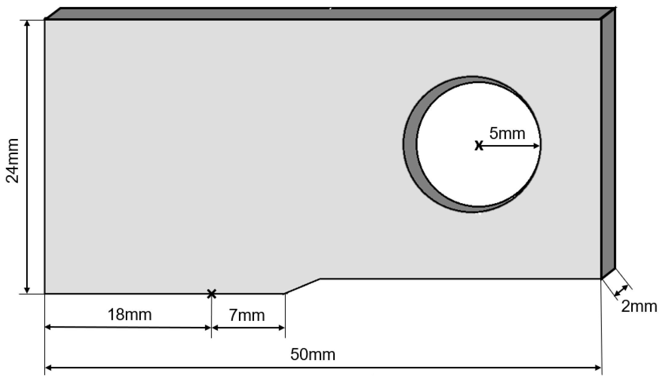
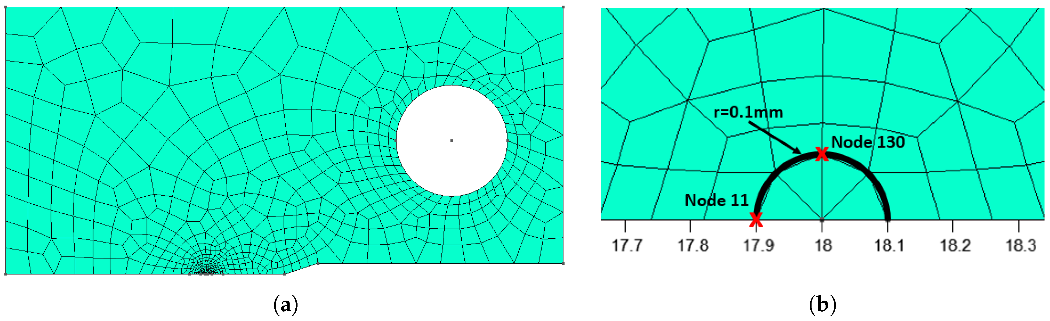
The CT specimen’s dimensions following the ASTM E 647-08 standard and an illustrative drawing, with the respective dimension values, are presented in Figure 2. With respect to this part, a mesh was designed, which is shown in Figure 3a. Although this mesh does not possess a structured form, the obtained results should be accurate enough for this purpose, even more so due to the small dimensions of the elements near the crack tip area, which is the area of most interest. The mesh refinement was performed using the same method as in other studies [9,37]. As the orthotropic characteristic is one of the points of focus, the analysis is centered a lot around two specific nodes near the crack tip, node 11 and node 130, presented in Figure 3b. Both nodes are at the same distance from the crack tip, mm, so there are no major differences when comparing the results.
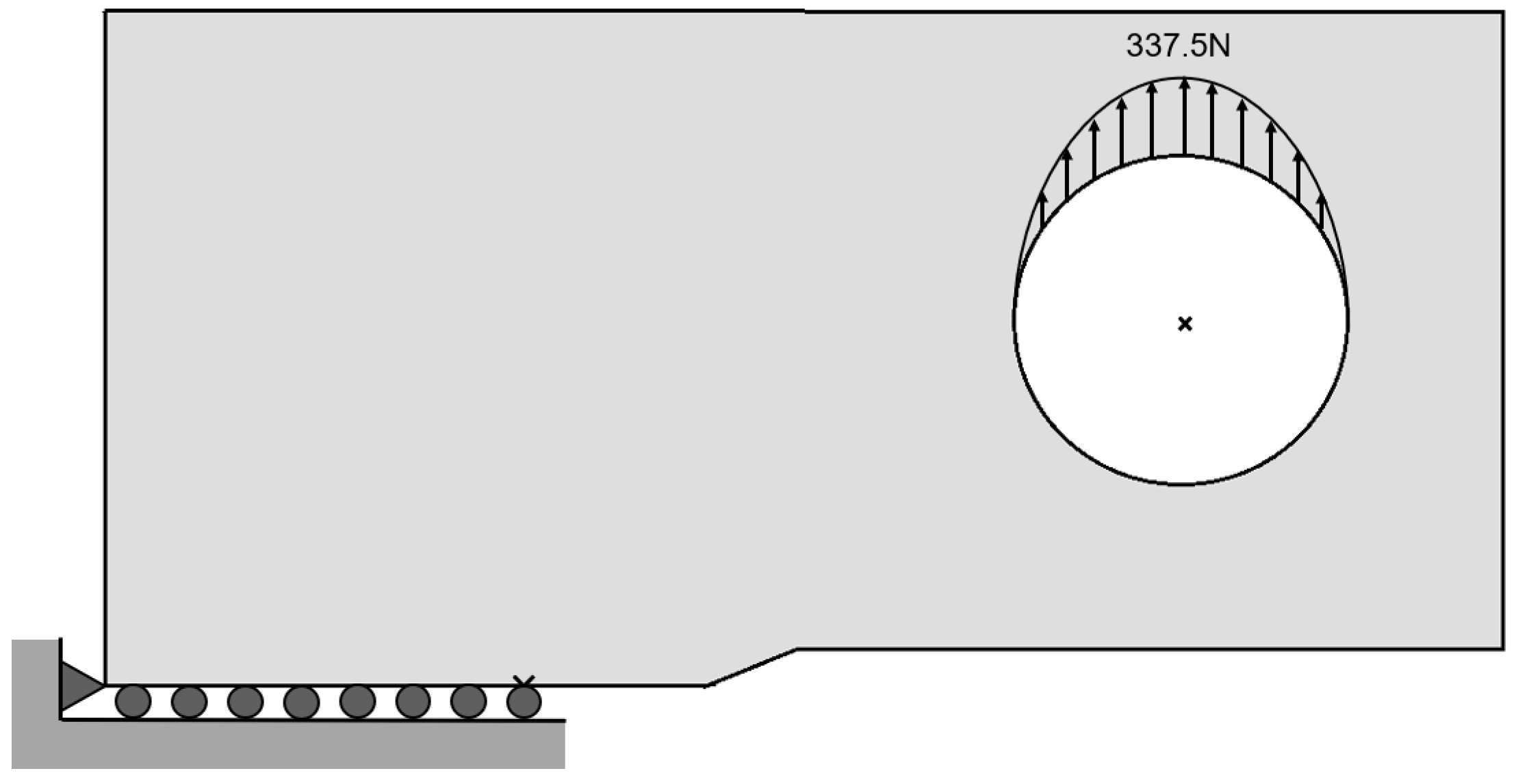
To perform the elastic simulations, boundary conditions have to be known. The boundary conditions considered are illustrated in Figure 4. Those were applied by differing various types of nodes:
- Node type 0—free movement and no load applied.
- Node type 1—free movement and load applied.
- Node type 2—constrained movement in the y direction and no load applied.
- Node type 3—constrained movement in both directions and no load applied.
A fixed node (node type 3) is necessary to prevent the parts free movement, that being the bottom left corner one. It is worth noting that the distributed load applied assumes a parabola-type behavior, as can be observed in Figure 4. Regarding the thermal simulation, the boundary conditions applied relate to the convection, and that was only applied at the boundary nodes, as already explained.
3.2. Single Lap Joint
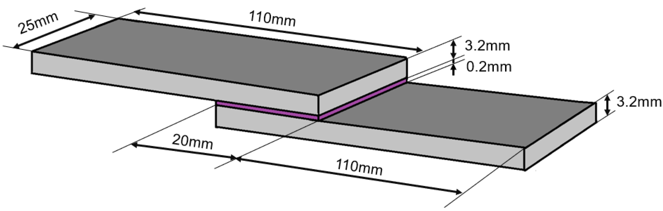
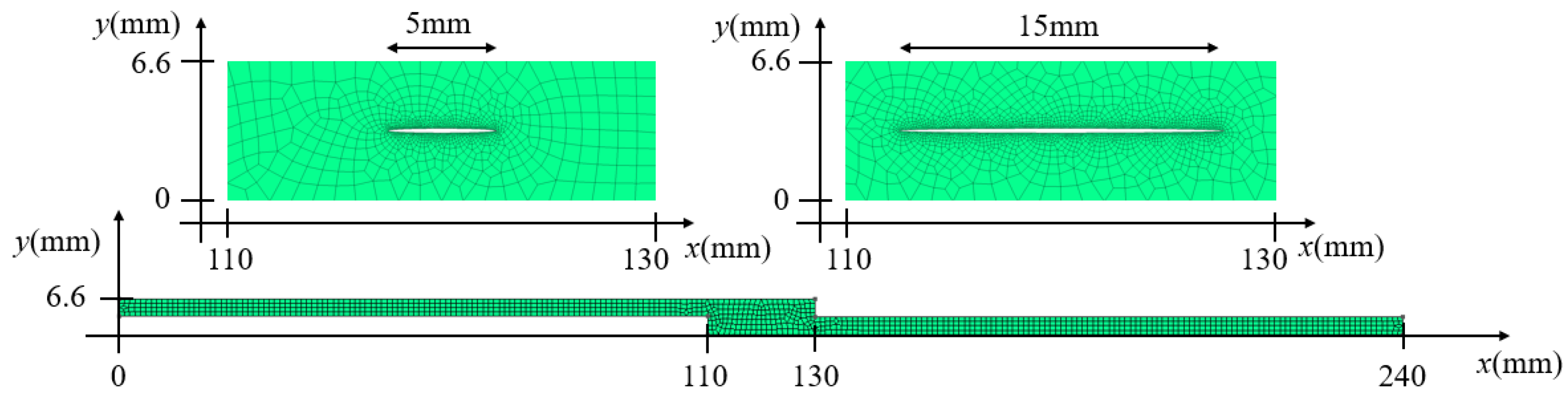
Regarding the SLJ, the dimensions, boundary conditions, and material properties were based on the work done in [38]. All the dimensions used in this SLJ specimens are presented in the illustration of Figure 5; the x and y directions being as represented in Figure 6, and the z direction represents the direction of the thickness. According to the figure shown, mm, mm, and mm. Differently from [38], we added a defect to this part, more specifically, an air bubble in the resin layer that connected both carbon fiber reinforced plastic (CFRP) plates, in the middle of the specimen, in order to study the potential of the TSA technique for detecting failures in composite materials. When designing the mesh, the air bubble was taken in account, and so, three identical meshes were designed, changing only in the length of the defect, called mesh 1, mesh 2, and mesh 3, respectively. The meshes were designed considering a middle plane at mm. Mesh 1 has no defect present, for comparison purposes. The bubble was considered an ellipse, and since the layer of resin was only mm thick, the radius in the y direction was kept constant ( mm). The value of the radius in the x direction: mm for mesh 2 and mm for mesh 3. Since the three meshes were identical, only mesh 1 is fully presented at the bottom of Figure 6. At the top of the figure, the zooms around the defect for mesh 2 and mesh 3 are presented. The meshes, away from the air bubble, had a structured form, and near it the, element was small enough and should produce good results.
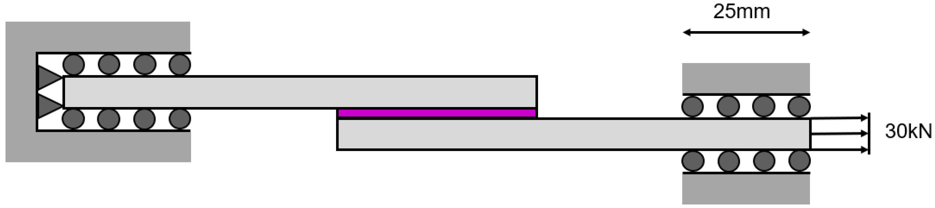
When it comes to the boundary conditions applied, the method applied was the same as to the CT specimen, i.e, considering the same different node types. A schematic illustration of the applied boundary conditions is presented in Figure 7. The restriction in the y direction that can be observed at the end of the plates corresponds to an alignment tab.
To perform the simulations, the material properties were needed, and so simplifications were made. It was to consider the part as one and made from the same material: an CFRP/epoxy composite (only the values for the Young’s modulus and Poisson’s coefficient are relative to a ply of CFRP) with the properties extracted from [5,38,39], which are presented in Table 1 and Table 2. It was considered that the Poisson’s ratio was the same in all directions and the yield strength used was an average value, which was considered constant as well in all directions.
4. Results
4.1. CT Specimen
The first test that was performed consisted in considering an isotropic material (in this case, aluminum 2219-T851). This means that the properties were the same in both x and y directions, and as presented in Table 3. Additionally, this means that Equation (14) was used with for the case of aluminum.
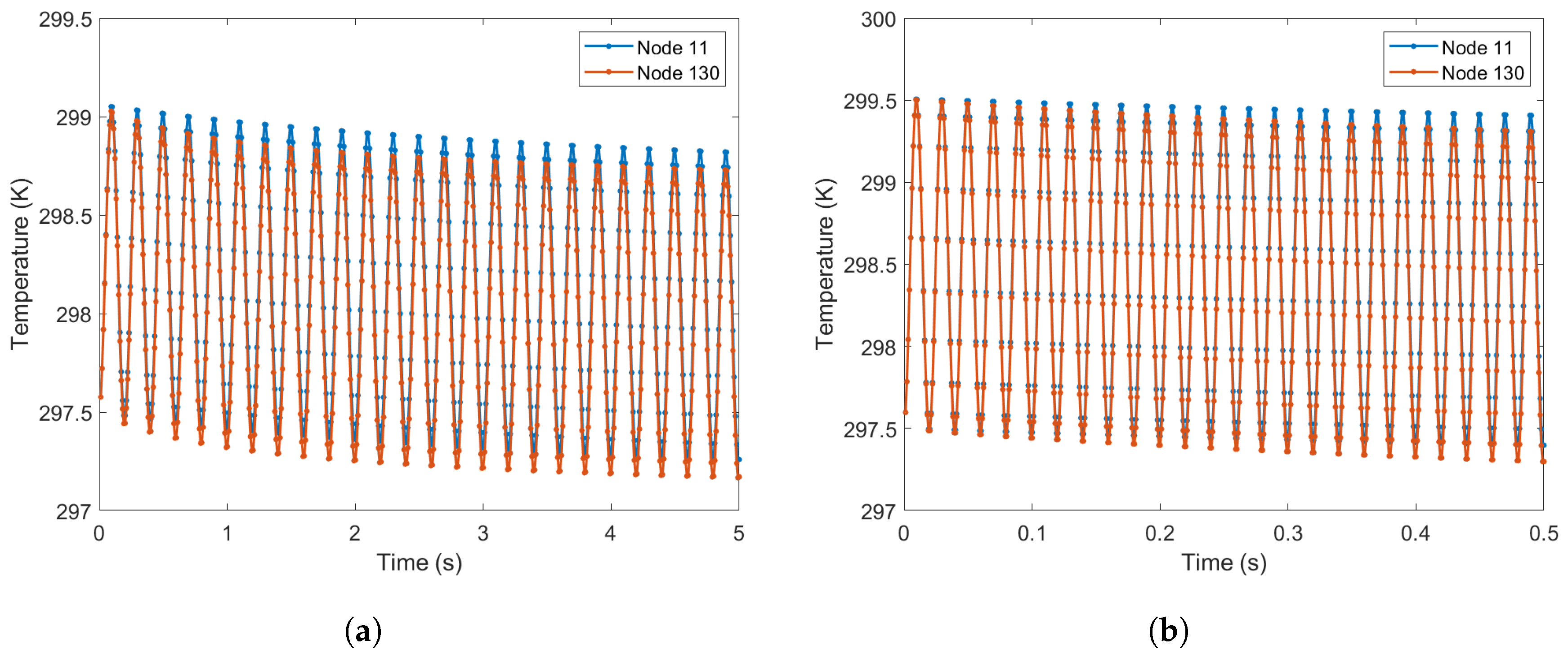
The goal of this first analysis was to understand the effect of conductivity, and so the thermal conductivity value was changed in each simulation performed to one the values presented in Table 4. The magnitude of differences between the chosen values was large in order to really see the effect of this parameter. After these first simulations were done, the temperature variation with time was plotted for both above-referenced nodes. As the lower conductivity values produced nearly no effect on the temperature variation, remaining almost constant, only the plots of the highest conductivity values are shown in Figure 8a,b.
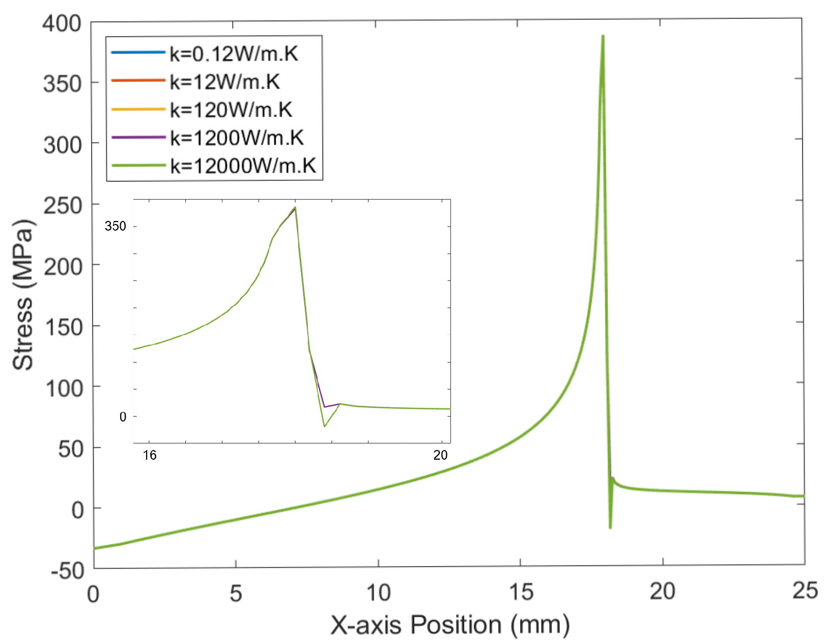
Besides these graphics, the stress profile along the symmetry axis is also plotted, see Figure 9, with a zoom around the crack tip area.
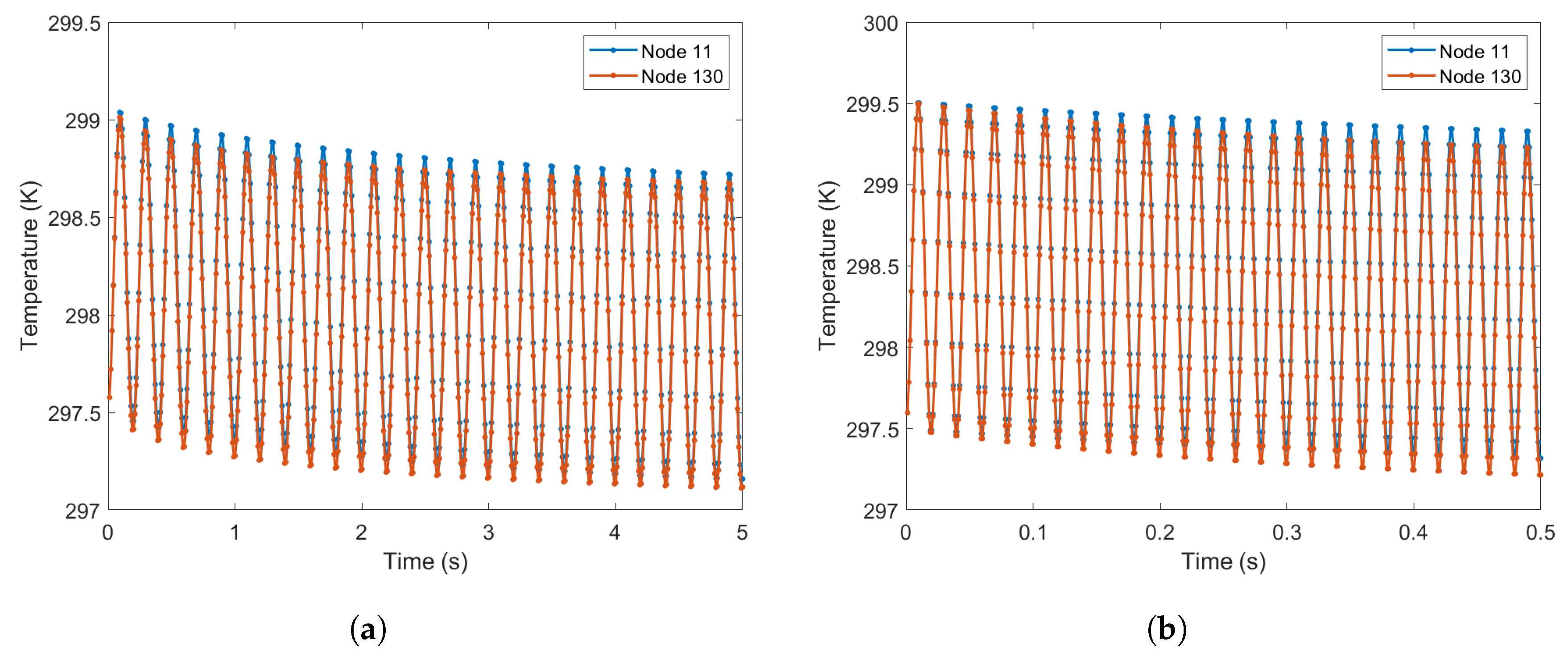
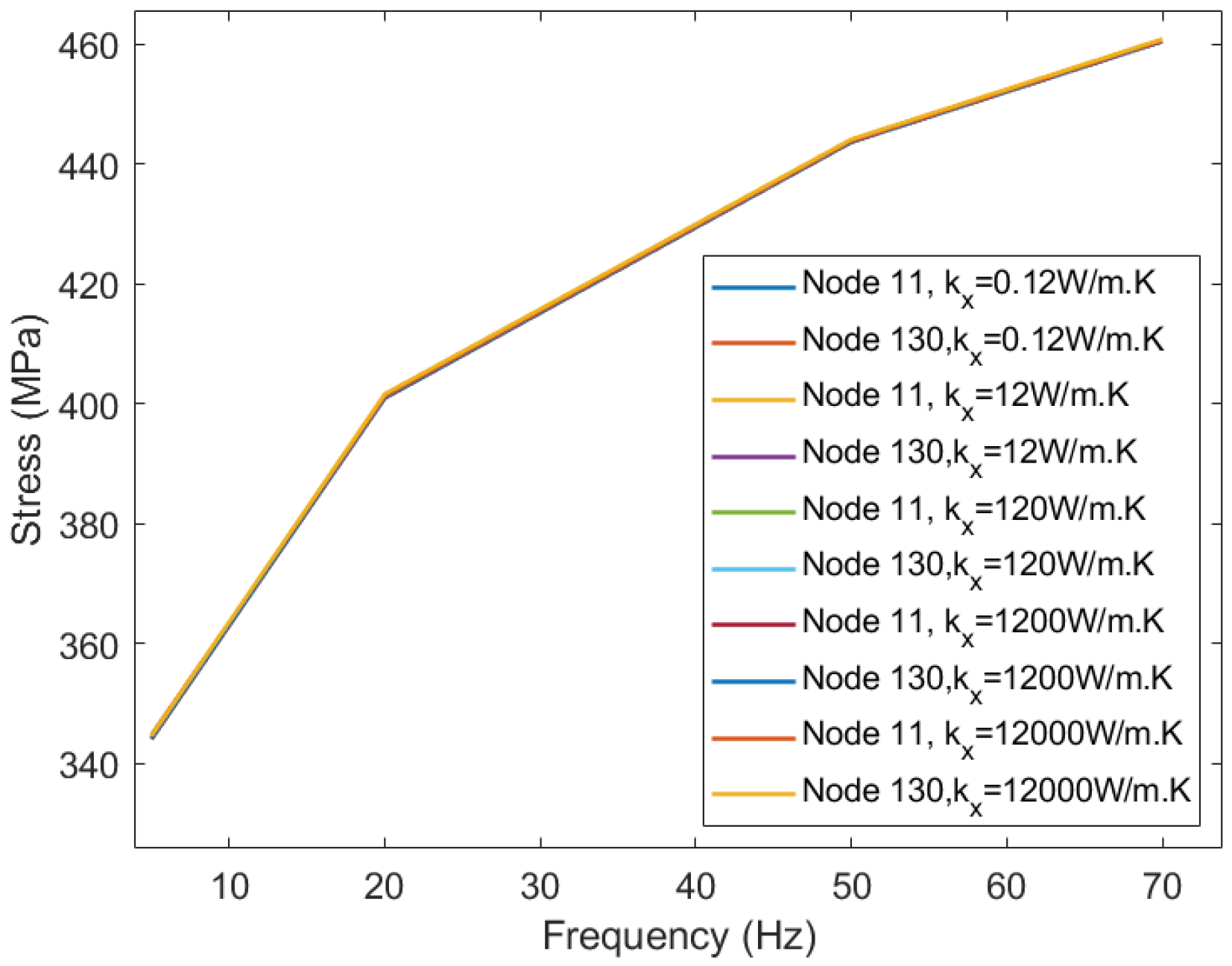
The second experiment that was conducted had the objectives of: (a) seeing if the model was property simulating the different values in the two directions; (b) analyzing the effect of having different conductivity’s in x and y directions. To realize these simulations, all properties used were the same as before; only the conductivity in the x direction, , was changed, to the values presented in Table 4. As before, the temperature variation with time was plotted for different cases, as shown in Figure 10a,b. As explained above, only the plots containing relevant information are shown. The obtained stress as a function of the loading frequency was also plotted—presented in Figure 11. This graphic was plotted for both node 11 and 130, since the values should be different for the two cases.
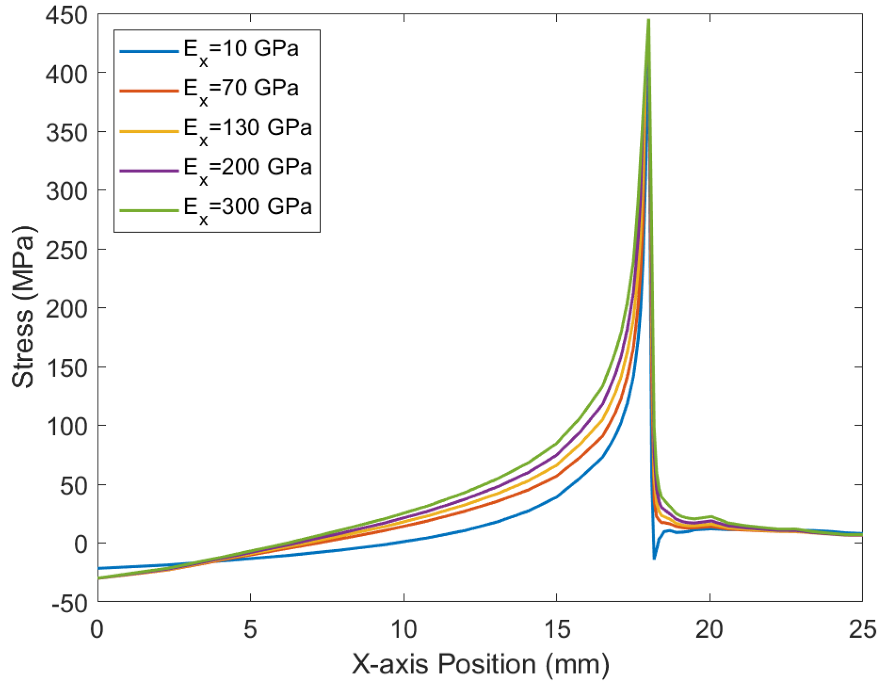
A third test was performed considering only orthotropical elastic properties. The previous experiments focused only on the conductivity. Thus, the main goal of this test was to access the effect that variation in the elastic properties has on the simulations. To achieve this goal, the simulations were run considering the same properties presented in Table 3; however, the Young’s modulus in the x direction, , was changed in each simulation. The values chosen are presented in Table 5. Just as before, the differences in the selected values were large in order to accentuate the changes from each simulation.
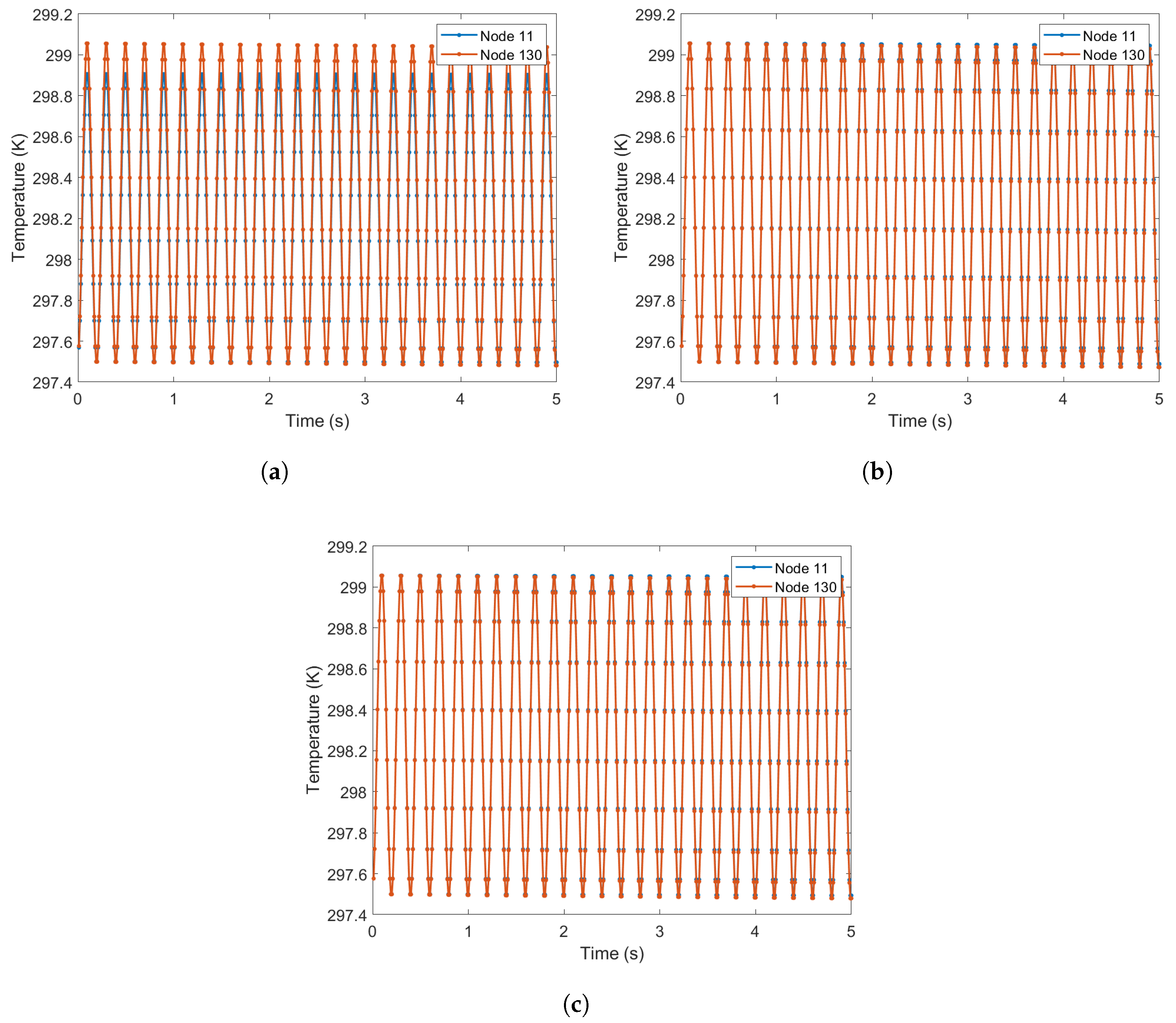
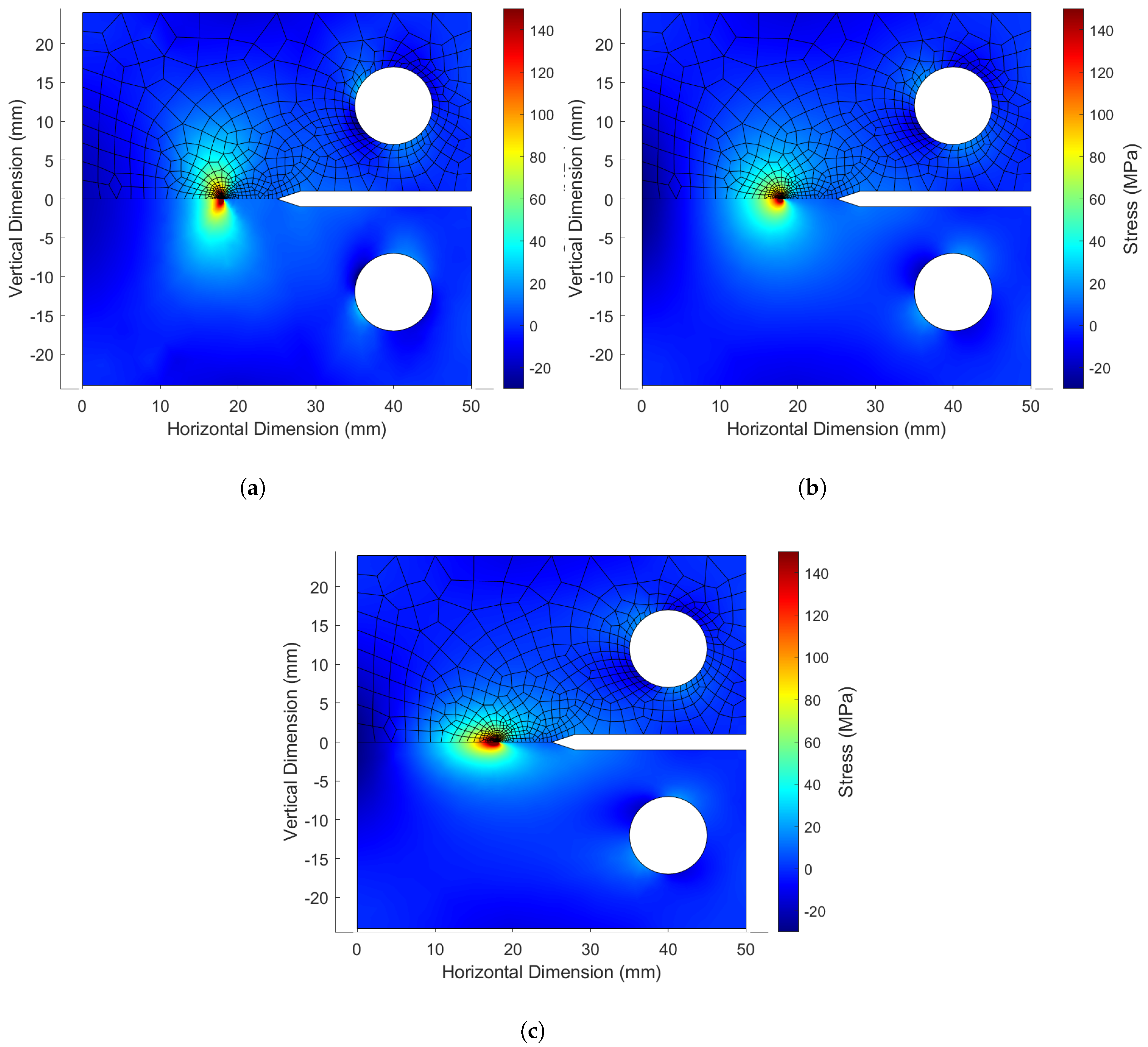
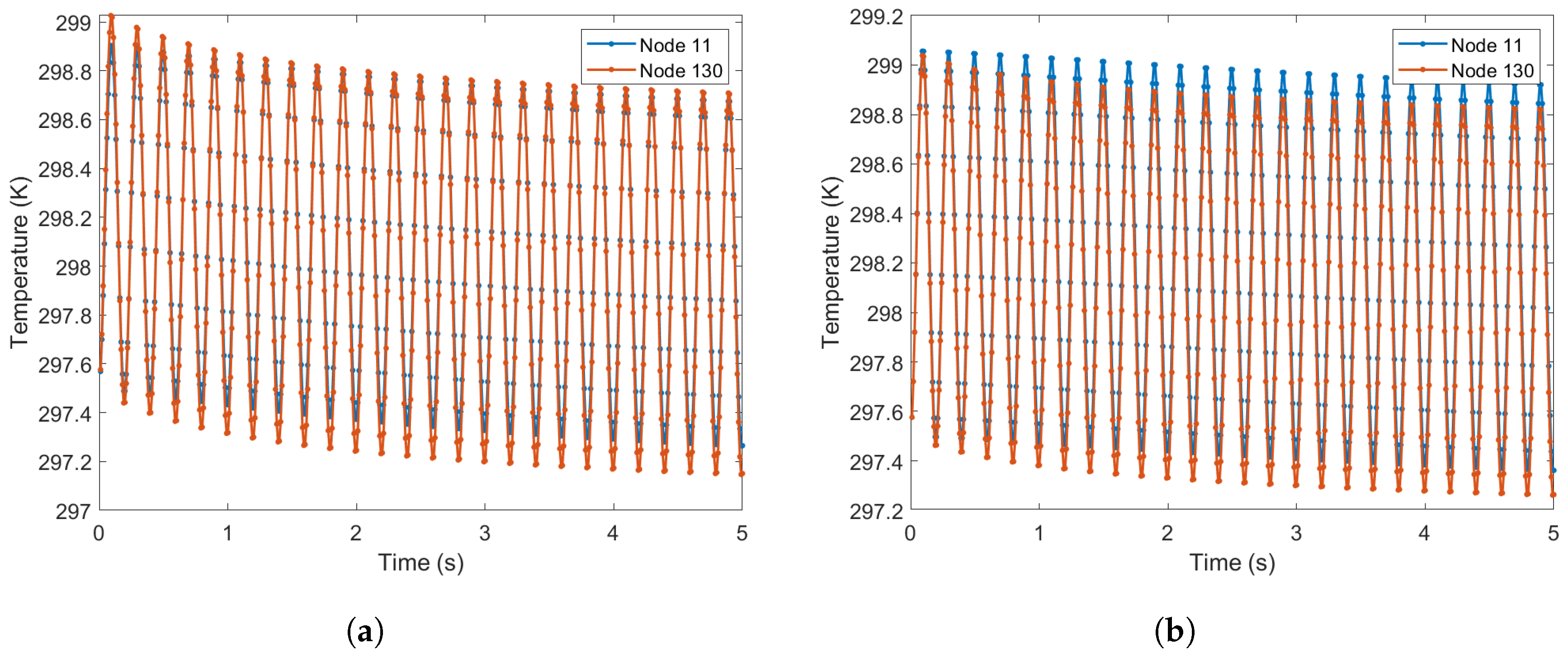
The temperature’s variation with time was once again plotted, for the cases of interest, and is shown in Figure 12a–c. Similarly to what was shown before, stress profiles along the symmetry axis were also plotted; see Figure 13. Finally, a stress distribution map was traced for each case, to make more noticeable the effect of the change in elastic properties. These maps are illustrated in Figure 14a–c.
The fourth and final experiment realized in the simulations using the CT specimen combined changes in conductivity and elastic properties, to see how these two aspects would affect the TSA simulation together. All properties remained constant with the same values as before, while varying only and using the values presented in Table 4 and Table 5, respectively.
The temperature’s variation with time was plotted for every case tested. However, due to there being too much information and much irrelevant data, since the effects of both could already be seen from the previous tests, only two plots are presented for the most extreme cases simulated; see Figure 15a,b. Other data, such as stress plots and distribution maps, are not shown either, due to the same reason.
4.2. Single Lap Joint
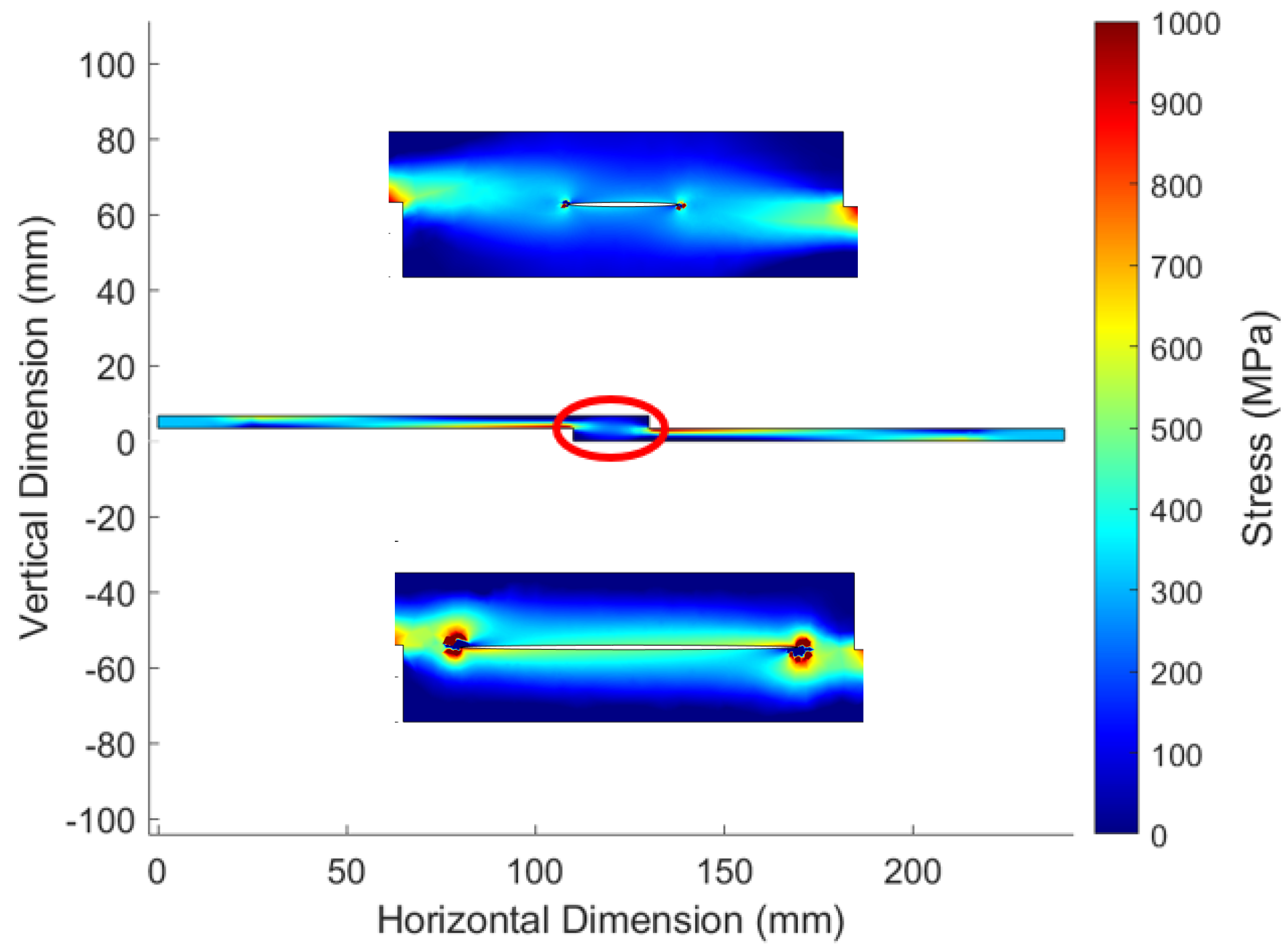
The SLJ specimen was submitted to TSA simulation with a loading frequency of 20 Hz. The three meshes were tested. The overall stress distribution maps are very similar; only in the area around the defect changes. Thus, the global TSA stress distribution map is only presented for mesh 1, but the stress distribution around the defect is present for both mesh 2 and mesh 3; see Figure 16.
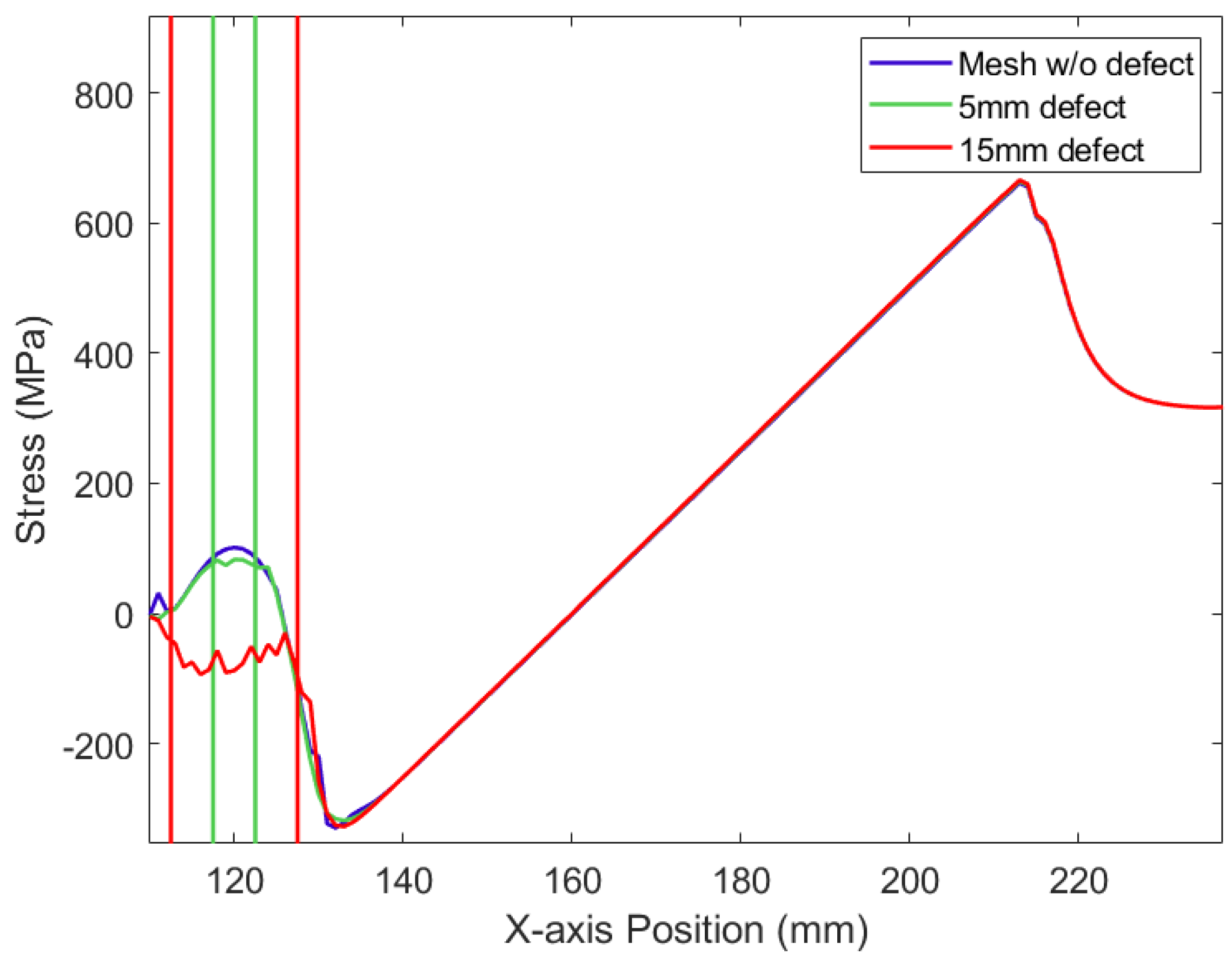
As the TSA technique only allows surface measurements, the stress analysis on one of the two plies surfaces was of most interest. Therefore, the stress profile along the bottom surface of the bottom ply was plotted for the three different meshes, as presented in Figure 17. The vertical lines correspond to the beginning and end of the defect, for the respective mesh, with the center of the defect being at mm.
5. Discussion
When considering an orthotropic material, and comparing the temperature variations obtained for two different frequencies, 5 and 50 Hz, in Figure 8a and Figure 8b, respectively, it is noticeable that loading frequency has an effect on the conductivity, as shown by the more clear temperature signal attenuation at low frequencies, just as was expected, since with higher frequencies, heat has less time to propagate. Besides this, a further look at these two plots can reveal that nodes 11 and 130 have the same attenuation, although the temperature values are a little lower in the vertical direction. When it comes to the conductivity value itself, a little attenuation is noticeable at the W/m·K, growing bigger when increasing this value. When analyzing the stress profiles plotted in Figure 9, it can be seen that the change in the conductivity values barely affects the stress values obtained, because although the attenuation of the temperature signal is altered, its amplitude remains nearly the same. Thus, this is not responsible for the thermal patterns observed by different frequencies.
In the second test, the conductivity value remained constant in the y direction, and it was changed at each simulation for the x direction. As for the case of W/m·K, the effects are more noticeable; that was the case used for analysis—see Figure 10a,b. For this case, it was expected that at node 11, the conductivity effect would be more accentuated than at node 130. However, it seems that was not the case. Actually, when comparing to the isotropic case shown before, the results are very similar. Regarding the stress plot for different loading frequencies, Figure 11, it is observable that the different values and cases have no clear effect on the stress behavior with the loading frequency. This raises the question, what is the influence of the frequency on the TSA results? This issue was reported in previous works by the authors [14] and requires deeper research. This was the case not only for mode I but also for mode II and mode III. Looking at the TSA theory, the load frequency is not considered an influencing parameter. The results presented here, and the experimental ones obtained previously, indicate that this consideration is incomplete. As such, it is imperative that future research tackles this issue in full detail, especially for when the TSA is used with high stress values and high stress gradients.
Regarding the changes in Young’s modulus, its effects can be clearly seen by looking at the obtained stress distribution maps. Compared to the isotropic case, Figure 14b, where the stress distribution has a heart shape, the decrease in Young’s modulus in the x direction tightens in this form, Figure 14a, and the increase in this value stretches across this stress distribution, Figure 14c. These changes are also visible when analyzing the stress profiles; see Figure 13. However, is also noticeable that the stresses near the crack tip tend practically to the same values. This was expected, since the mesh used for the simulations was the same, and so it is normal that the plots tend to have the same value. When looking at the temperature variations, Figure 12a–c, it is clear that these changes only affect the amplitude of the signal, as expected. Still, the differences between the temperature plot for GPa and for GPa are almost nonexistent for node 11, although the difference in values is big. This also proves the tendency for the same stress values around the crack tip.
The fourth and last test, varying both conductivity and Young’s modulus in the x direction, was more proof of what was concluded from the previous tests. The temperature variations observed in Figure 15a,b show the expected behavior considering the above-presented discussion.
Finally, the created TSA model was tested with a composite material and applied to the SLJ specimen. The main goal of this simulation was to evaluate if the TSA technique could be used to detect the presence of defects, such as delamination, in these types of materials. The stress distribution maps obtained, Figure 16, were as expected, with the stress concentrations being bigger as the defect grew bigger. However, there are some areas, specifically around the defect tips, where the stress distribution has sudden stress changes. This is due to the discretization process inherent in the FEM. Different meshes will produce different results, but with similar patterns. For this reason, the TSA measures and high-stress analysis should be performed in areas without stress concentration. An alternative and future work will be to perform the simulations using meshless techniques. Since the technique allows surface measurement, the stress profile on the surface of the bottom ply was plotted in Figure 17. By analyzing these plots overall, it can be seen that the defect presence is noted in the surface stress profiles obtained with the TSA simulation. The presence of the defect deviates from the stress values when compared to the simulation without the defect. It can be concluded that the bigger the defect, the more detectable the presence of the defect. The exact locations of the beginning and the end of the defect are not precise, but a good estimation can be made. The detection of it is noticeable, meaning that TSA is capable of detecting the presence of a defect in composite materials.
The model conceived in this work was based on experimental tests performed with a FLIR SC7500. This camera has an NEDT (noise equivalent differential temperature) of less than 25 mK. As such, and at the current time, the authors cannot guarantee that errors in the simulations are smaller than 25 mK. Assuming the behaviors such as other applications of lock-in processing and similar test conditions, the errors between the simulations and the inferred laboratory conditions are expected to be smaller than 1.0 mK for both CT and SLJ. This is based on the authors’ experience.
6. Conclusions
This work had the main goal of creating a computational model based on the finite element method that simulates TSA applied to orthotropic materials, in order to study the effects of the material’s properties on the results and to evaluate the application of this technique to different materials, including composites. The methodology based on FEM was presented firstly. Then, the model was used on a CT specimen; the results helped to better understand the effects of the material’s properties and changes in its values. Finally, an SLJ specimen was simulated by the model. It was composed of a composite orthotropic material, so the potential of the application of the present model was tested. The simulations done showed that defect detection is possible with this technique.
As a final remark, the created model acceptably reproduced the TSA technique. The simulations helped to better understand material’s properties’ effects on the obtained results and to prove this technique’s potential for applications for orthotropic materials, including composites. However, there is still room for improvement and to perfect this model, especially considering the difficulty of the TSA analysis of these materials. Future works should consider anisotropic materials and the inherent concentration of stresses in certain areas, along with these areas’ effects on the material models and the TSA readings. Both numeric simulations and experimental testing should be involved.
Author Contributions
Methodology, A.R.S.; formal analysis, G.D., A.N. and A.R.S.; investigation, G.D.; writing—original draft, G.D.; writing—review & editing, A.N. and A.R.S.; supervision, A.N. All authors have read and agreed to the published version of the manuscript.
Funding
This research was funded by Fundação para a Ciência e a Tecnologia Project UIDB/50022/2020, UIDP/50022/2020.
Data Availability Statement
Not applicable.
Conflicts of Interest
The authors declare no conflict of interest.
Nomenclature
| [K] | Stiffness matrix (N mm) |
| {u} | Displacement vector (mm) |
| {F} | Load vector (N) |
| [B] | Strain matrix |
| [D] | Elasticity matrix (GPa) |
| [J] | Jacobian matrix |
| (, ) | Isoparametric coordinates |
| Variable x at Gauss point | |
| Young’s modulus in the i direction (GPa) | |
| Poisson’s ratio in the i and j directions | |
| External forces applied over the element area (N mm) | |
| Surface traction forces (N mm) | |
| Strain vector | |
| Stress vector (MPa) | |
| T | Temperature (K) |
| t | Time (s) |
| Derivative of variable x with respect to time | |
| [C] | Mass matrix (kg) |
| Heat vector (W) | |
| k | Thermal conductivity () |
| Density (kg m) | |
| Specific heat capacity at constant pressure () | |
| h | Convection coefficient () |
| f | Frequency (Hz) |
| Period (s) | |
| n | Number of cycles |
| Maximum number of increments | |
| Thermal expansion coefficient in the i direction (K) |
References
- La Rosa, G.; Risitano, A. Thermographic methodology for rapid determination of the fatigue limit of materials and mechanical components. Int. J. Fatigue 2000, 22, 65–73. [Google Scholar] [CrossRef]
- Luong, M.P. Fatigue limit evaluation of metals using an infrared thermographic technique. Mech. Mater. 1998, 28, 155–163. [Google Scholar] [CrossRef]
- Wang, X.; Crupi, V.; Jiang, C.; Feng, E.; Guglielmino, E.; Wang, C. Energy-based approach for fatigue life prediction of pure copper. Int. J. Fatigue 2017, 104, 243–250. [Google Scholar] [CrossRef]
- Laguela, S.; Martínez, J.; Armesto, J.; Arias, P. Energy efficiency studies through 3D laser scanning and thermographic technologies. Energy Build. 2011, 43, 1216–1221. [Google Scholar] [CrossRef]
- Tian, T.; Cole, K.D. Anisotropic thermal conductivity measurement of carbon-fiber/epoxy composite materials. Int. J. Heat Mass Transf. 2012, 55, 6530–6537. [Google Scholar] [CrossRef]
- Villière, M.; Lecointe, D.; Sobotka, V.; Nicolas, B.; Delaunay, D. Experimental determination and modeling of thermal conductivity tensor of carbon/epoxy composite. Compos. Part A Appl. Sci. Manuf. 2013, 46, 60–68. [Google Scholar] [CrossRef] [Green Version]
- Strzałkowski, K.; Streza, M.; Pawlak, M. Lock-in thermography versus PPE calorimetry for accurate measurements of thermophysical properties of solid samples: A comparative study. Measurement 2015, 64, 64–70. [Google Scholar] [CrossRef]
- António Ramos, S.; Vaz, M.; Leite, S.R.; Mendes, J. Non-Destructive Infrared Lock-in Thermal Tests: Update on the Current Defect Detectability. Russ. J. Nondestruct. Test. 2019, 55, 772–784. [Google Scholar] [CrossRef]
- Ramos Silva, A.J.; Vaz, M.; Ribeirinho Leite, S.; Mendes, J. Analyzing the Influence of the Stimulation Duration in the Transient Thermal Test—Experimental and FEM Simulation. Exp. Tech. 2022. [Google Scholar] [CrossRef]
- Silva, A.R.; Vaz, M.; Leite, S.; Gabriel, J. Lock-in thermal test with corrected optical stimulation. Quant. Infrared Thermogr. J. 2022, 19, 261–282. [Google Scholar] [CrossRef]
- Ramos Silva, A.; Vaz, M.; Ribeirinho Leite, S.; Mendes, J. Analyzing the influence of thermal NDT parameters on test performance. Russ. J. Nondestruct. Test. 2021, 57, 727–737. [Google Scholar] [CrossRef]
- Sharpe, W.N., Jr. Springer Handbook of Experimental Solid Mechanics; Springer Handbooks: Berlin/Heidelberg, Germany, 2008. [Google Scholar]
- An, Y.K.; Min Kim, J.; Sohn, H. Laser lock-in thermography for detection of surface-breaking fatigue cracks on uncoated steel structures. NDT E Int. 2014, 65, 54–63. [Google Scholar] [CrossRef]
- Silva, A.J.R.; Moreira, P.M.G.; Vaz, M.A.P.; Gabriel, J. Temperature profiles obtained in thermoelastic stress test for different frequencies. Int. J. Struct. Integr. 2017, 8, 51–62. [Google Scholar] [CrossRef]
- Farahani, B.V.; de Melo, F.Q.; Tavares, P.J.; Moreira, P.M. New approaches on the stress intensity factor characterization—Review. Procedia Struct. Integr. 2020, 28, 226–233. [Google Scholar] [CrossRef]
- Ancona, F.; De Finis, R.; Palumbo, D.; Galietti, U. Crack Growth Monitoring in Stainless Steels by Means of TSA Technique. Procedia Eng. 2015, 109, 89–96. [Google Scholar] [CrossRef] [Green Version]
- Díaz, F.A.; Patterson, E.A.; Tomlinson, R.A.; Yates, J.R. Measuring stress intensity factors during fatigue crack growth using thermoelasticity. Fatigue Fract. Eng. Mater. Struct. 2004, 27, 571–583. [Google Scholar] [CrossRef]
- Díaz, F.A.; Vasco-Olmo, J.M.; López-Alba, E.; Felipe-Sesé, L.; Molina-Viedma, A.J.; Nowell, D. Experimental evaluation of effective stress intensity factor using thermoelastic stress analysis and digital image correlation. Int. J. Fatigue 2020, 135, 105567. [Google Scholar] [CrossRef]
- Díaz, F.A.; Yates, J.R.; Patterson, E.A. Some improvements in the analysis of fatigue cracks using thermoelasticity. Int. J. Fatigue 2004, 26, 365–376. [Google Scholar] [CrossRef]
- Duarte, G.; Neves, A.M.A.; Silva, A.J.R. Temperature patterns obtained in thermoelastic stress test for different frequencies, a FEM approach. Submitt. Int. J. Struct. Integr. 2022, in press.
- Kakei, A.; Epaarachchi, J.A.; Islam, M.; Leng, J.; Rajic, N. Detection and characterisation of delamination damage propagation in Woven Glass Fibre Reinforced Polymer Composite using thermoelastic response mapping. Compos. Struct. 2016, 153, 442–450. [Google Scholar] [CrossRef] [Green Version]
- Kakei, A.; Epaarachchi, J.A.; Islam, M.; Leng, J. Evaluation of delamination crack tip in woven fibre glass reinforced polymer composite using FBG sensor spectra and thermo-elastic response. Meas. J. Int. Meas. Confed. 2018, 122, 178–185. [Google Scholar] [CrossRef]
- Jiménez-Fortunato, I.; Bull, D.J.; Thomsen, O.T.; Dulieu-Barton, J.M. On the source of the thermoelastic response from orthotropic fibre reinforced composite laminates. Compos. Part A Appl. Sci. Manuf. 2021, 149, 106515. [Google Scholar] [CrossRef]
- Mackin, T.; Roberts, M. Evaluation of Damage Evolution in Ceramic-Matrix Composites Using Thermoelastic Stress Analysis. J. Am. Ceram. Soc. 2004, 83, 337–343. [Google Scholar] [CrossRef]
- Palumbo, D.; De Finis, R.; Di Carolo, F.; Vasco-Olmo, J.; Diaz, F.A.; Galietti, U. Influence of Second-Order Effects on Thermoelastic Behaviour in the Proximity of Crack Tips on Titanium. Exp. Mech. 2022, 62, 521–535. [Google Scholar] [CrossRef]
- De Finis, R.; Palumbo, D.; Galietti, U. Evaluation of damage in composites by using thermoelastic stress analysis: A promising technique to assess the stiffness degradation. Fatigue Fract. Eng. Mater. Struct. 2020, 43, 2085–2100. [Google Scholar] [CrossRef]
- Di Carolo, F.; De Finis, R.; Palumbo, D.; Galietti, U. Study of the thermo-elastic stress analysis (TSA) sensitivity in the evaluation of residual stress in non-ferrous metal. In Thermosense: Thermal Infrared Applications XLI; SPIE: Bellingham, WA, USA, 2019; p. 25. [Google Scholar] [CrossRef]
- Di Carolo, F.; De Finis, R.; Palumbo, D.; Galietti, U. A Thermoelastic Stress Analysis General Model: Study of the Influence of Biaxial Residual Stress on Aluminium and Titanium. Metals 2019, 9, 671. [Google Scholar] [CrossRef] [Green Version]
- Pitarresi, G.; Found, M.; Patterson, E. An investigation of the influence of macroscopic heterogeneity on the thermoelastic response of fibre reinforced plastics. Compos. Sci. Technol. 2005, 65, 269–280. [Google Scholar] [CrossRef]
- Thompson, E.G. A Introduction to the Finite Element Method: Theory, Programming and Applications; Wiley: Hoboken, NJ, USA, 2005; p. 360. [Google Scholar]
- Pires, F.M.A.; Carneiro, A.M.C.; Lopes, I.A.R. Finite Element Method Theoretical Classes. 2021. Available online: https://sigarra.up.pt/feup/pt/conteudos_adm.list?pct_pag_id=249640&pct_parametros=pv_ocorrencia_id=335032 (accessed on 16 October 2022).
- Donadon, M.; de Almeida, S. 2.07—Damage modeling in composite structures. In Comprehensive Materials Processing; Hashmi, S., Batalha, G.F., Van Tyne, C.J., Yilbas, B., Eds.; Elsevier: Amsterdam, The Netherlands, 2014; pp. 111–147. [Google Scholar] [CrossRef]
- Kitade, S.; Pullen, K. 3.20 Flywheel. In Comprehensive Composite Materials II; Beaumont, P.W., Zweben, C.H., Eds.; Elsevier: Amsterdam, The Netherlands, 2016; pp. 545–555. [Google Scholar] [CrossRef]
- Arfken, G.B.; Griffing, D.F.; Kelly, D.C.; Priest, J. (Eds.) Chapter 23—Heat Transfer. In International Edition University Physics; Academic Press: Cambridge, MA, USA, 1984; pp. 430–443. [Google Scholar] [CrossRef]
- Hillel, D. Soil physics. In Encyclopedia of Physical Science and Technology, 3rd ed.; Meyers, R.A., Ed.; Academic Press: Cambridge, MA, USA, 2001; pp. 77–97. [Google Scholar] [CrossRef]
- Kosky, P.; Balmer, R.; Keat, W.; Wise, G. (Eds.) Chapter 12—Mechanical Engineering. In Exploring Engineering, 3rd ed.; Academic Press: Boston, MA, USA, 2013; pp. 259–281. [Google Scholar] [CrossRef]
- Ramos Silva, A.J.; Vaz, M.; Ribeirinho Leite, S.; Mendes, J. Lock-in Thermal Test Simulation, Influence, and optimum cycle period for infrared thermal testing in Non-destructive testing. Sensors 2023, 23, 325. [Google Scholar] [CrossRef]
- Santos, D.d.; Carbas, R.; Marques, E.; da Silva, L. Reinforcement of CFRP joints with fibre metal laminates and additional adhesive layers. Compos. Part B Eng. 2019, 165, 386–396. [Google Scholar] [CrossRef]
- MatWeb. Available online: https://www.matweb.com/search/datasheet_print.aspx?matguid=39e40851fc164b6c9bda29d798bf3726 (accessed on 6 September 2022).
- Kang, J.; Liang, S.; Wu, A.; Li, Q.; Wang, G. Local Liquation Phenomenon and Its Effect on Mechanical Properties of Joint in Friction Stir Welded 2219 Al Alloy. Jinshu Xuebao/Acta Metall. Sin. 2017, 53, 358–368. [Google Scholar] [CrossRef]
Figure 1.
Workflow of this work.

Figure 2.
Dimensions of the CT specimen.

Figure 3.
Mesh designed for the CT specimen. (a) Complete designed mesh. (b) Zoom in around the crack tip.
Figure 3.
Mesh designed for the CT specimen. (a) Complete designed mesh. (b) Zoom in around the crack tip.

Figure 4.
Boundary conditions applied to the CT specimen.

Figure 5.
Dimensions of the SLJ.

Figure 6.
Designed mesh for the SLJ with the respective zooms around the defect.

Figure 7.
Boundary conditions considered in the SLJ.

Figure 8.
Temperature variation with time in the specimen for different frequencies and conductivities. (a) Hz and W/m·K. (b) Hz and W/m·K.
Figure 8.
Temperature variation with time in the specimen for different frequencies and conductivities. (a) Hz and W/m·K. (b) Hz and W/m·K.

Figure 9.
Stress profiles for different conductivities.

Figure 10.
Temperature variation with time in the specimen for different frequencies and orthotropic conductivities. (a) Hz and W/m·K. (b) Hz and W/m·K.
Figure 10.
Temperature variation with time in the specimen for different frequencies and orthotropic conductivities. (a) Hz and W/m·K. (b) Hz and W/m·K.

Figure 11.
Plot of stress vs. frequency.

Figure 12.
Temperature variation with time in the specimen for various values of elastic properties and Hz. (a) GPa. (b) GPa. (c) GPa.
Figure 12.
Temperature variation with time in the specimen for various values of elastic properties and Hz. (a) GPa. (b) GPa. (c) GPa.

Figure 13.
Stress profiles for various values of elastic properties.

Figure 14.
TSA stress distribution maps for Hz and various values of elastic properties. (a) GPa. (b) GPa. (c) GPa.
Figure 14.
TSA stress distribution maps for Hz and various values of elastic properties. (a) GPa. (b) GPa. (c) GPa.

Figure 15.
Temperature variation with time in the specimen with Hz. (a) W/m·K and GPa. (b) W/m·K and GPa.
Figure 15.
Temperature variation with time in the specimen with Hz. (a) W/m·K and GPa. (b) W/m·K and GPa.

Figure 16.
TSA stress distribution map for the SLJ with the respective zooms around the defect.

Figure 17.
Stress profiles for the different meshes.


Table 1.
CFRP’s mechanical properties.
| Yield Strength (MPa) | (GPa) | (GPa) | Poisson’s Coefficient (-) | Density (kg/m3) |
|---|---|---|---|---|
| 1230 | 109 | 8.819 | 0.342 | 1410 |
Table 2.
CFRP’s thermal properties.
(W/m·K) | (W/m·K) | Specific Heat Capacity (J/kg·K) | ||
|---|---|---|---|---|
| 6.3 | 0.6 | 1130 | 21.3 | 67.6 |
Table 3.
Aluminum 2219-T851’s properties [40].
Table 3.
Aluminum 2219-T851’s properties [40].
| Yield Strength (MPa) | Young’s Modulus (GPa) | Poisson’s Coefficient (-) | Thermal Conductivity (W/m·K) | Density (kg/m ) | Specific Heat Capacity (J/Kg·K) |
|---|---|---|---|---|---|
| 352 | 73.1 | 0.33 | 120 | 2840 | 864 |
Table 4.
Thermal conductivity values for the performed test.
| Parameter | Value 1 | Value 2 | Value 3 | Value 4 | Value 5 |
|---|---|---|---|---|---|
| Thermal Conductivity (W/m·K) | 0.12 | 12 | 120 | 1200 | 12,000 |
Table 5.
Young’s modulus values for the tests.
| Parameter | Value 1 | Value 2 | Value 3 | Value 4 | Value 5 |
|---|---|---|---|---|---|
| Young’s Modulus (GPa) | 10 | 70 | 130 | 200 | 300 |
Disclaimer/Publisher’s Note: The statements, opinions and data contained in all publications are solely those of the individual author(s) and contributor(s) and not of MDPI and/or the editor(s). MDPI and/or the editor(s) disclaim responsibility for any injury to people or property resulting from any ideas, methods, instructions or products referred to in the content. |
© 2023 by the authors. Licensee MDPI, Basel, Switzerland. This article is an open access article distributed under the terms and conditions of the Creative Commons Attribution (CC BY) license (https://creativecommons.org/licenses/by/4.0/).
Share and Cite
MDPI and ACS Style
Duarte, G.; Neves, A.; Ramos Silva, A. Temperature Patterns in TSA for Different Frequencies and Material Properties: A FEM Approach. Math. Comput. Appl. 2023, 28, 8. https://doi.org/10.3390/mca28010008
AMA Style
Duarte G, Neves A, Ramos Silva A. Temperature Patterns in TSA for Different Frequencies and Material Properties: A FEM Approach. Mathematical and Computational Applications. 2023; 28(1):8. https://doi.org/10.3390/mca28010008
Chicago/Turabian StyleDuarte, Guilherme, Ana Neves, and António Ramos Silva. 2023. "Temperature Patterns in TSA for Different Frequencies and Material Properties: A FEM Approach" Mathematical and Computational Applications 28, no. 1: 8. https://doi.org/10.3390/mca28010008