An Adaptive in Space, Stabilized Finite Element Method via Residual Minimization for Linear and Nonlinear Unsteady Advection–Diffusion–Reaction Equations

Abstract

We construct a stabilized finite element method for linear and nonlinear unsteady advection–diffusion–reaction equations using the method of lines. We propose a residual minimization strategy that uses an ad-hoc modified discrete system that couples a time-marching schema and a semi-discrete discontinuous Galerkin formulation in space. This combination delivers a stable continuous solution and an on-the-fly error estimate that robustly guides adaptivity at every discrete time. We show the performance of advection-dominated problems to demonstrate stability in the solution and efficiency in the adaptivity strategy. We also present the method’s robustness in the nonlinear Bratu equation in two dimensions.

1. Introduction

The unsteady advection–diffusion–reaction model system poses distinct challenges for its numerical approximation. A limit case of interest arises when the equation becomes advection-dominated, showing sharp internal or boundary layers. Classical numerical methods (e.g., standard FEM) lead to numerical instabilities when the mesh is not sufficiently fine to capture the fine scales associated with these flow features, leading to unphysical oscillation.

Stabilized methods, such as Stream Upwind Petrov Galerkin (SUPG) [1] or Galerkin least squares (GLS) [2], overcome this problem by including artificial diffusion in the governing equation’s variational form. The variational multi-scale method (VMS) [3,4] captures fine-scale features by modifying the variational form [5,6,7,8]. Other technics such as the discontinuous Galerkin (dG) methods [9,10,11,12,13] stabilize the solution by providing local conservation and adding inner penalization across the element interfaces.

Methods based on residual minimization, including Least-Squares Finite Element Methods (LSFEM) and the Discontinuous Petrov–Galerkin method (DPG), seek stability by minimizing the discrete residual in dual norms [14,15,16]. Extensions to these ideas regarding parabolic problems include: [17,18,19,20] for dG and [14,21,22,23,24] for DPG methods.

Although these methods show stability for advection-dominated problems, the lack of a priori localization of the inner or boundary layers in the exact solution leads to expensive simulations on quasi-uniform meshes. Additionally, the lack of robust refinement strategies is critical for unsteady problems where the solution varies in space and time. Thus, we reduce this computational cost by using adaptive methods that rely on a posteriori error estimators to refine solution singularities. Posteriori error estimators for unsteady diffusion advection reaction methods are described in [25,26] and for unsteady dG implementations in [27,28,29].

Recently, Calo et al. [30] introduced a new class of adaptive stabilized conforming finite elements via residual minimization for steady problems. The method combines residual minimization ideas with the stability of the discontinuous Galerkin formulations. As a result, the method delivers a stable continuous solution and a robust error representation to perform on-the-fly adaptivity. The authors introduce the framework in a series of papers for linear and nonlinear applications (e.g., advection–diffusion problems with heterogeneous and highly anisotropic diffusion [31], its use combined with isogeometric analysis [32], nonlinear weak constraint enforcement [33], goal-oriented adaptivity [34], for incompressible flows [35,36], flow in porous media [37], and dynamic fracture propagation [38]).

In this paper, we extend [30] for unsteady advection–diffusion–reaction problems using the method of lines. Our method offers robust spatial refinements for a user-selected time marching method. We first approximate the spatial derivatives using a space semi-discrete scheme and then solve the resulting system using a time-marching discretization. As particular examples, this paper uses implicit first- and second-order time-stepping (BDF1 and BDF2) discretizations [39,40,41].

Compared to other techniques, the main advantage of this method relies on the non-conformity of the starting dG formulation, which allows us to work with stronger norms from the dG theory with a continuous trial space. Moreover, the refinement strategy and its efficiency in obtaining high-resolution approximations from coarse meshes allow us to overcome the computational cost resulting from the implicit temporal schemes and the extra degrees of freedom in the saddle point formulation.

The paper’s outline follows: Section 2 introduces the model problem. Section 3 describes some preliminary concepts for dG discretizations for time marching. Then, we present the well-posedness of the dG method combined with the backward differentiating formula for time marching. Section 4 describes the residual minimization problem and introduces our adaptive stabilized finite element method for parabolic problems. Finally, Section 5 contains some numerical examples showing uniform and adaptive refinement cases for two-dimension linear and non-linear problems, followed by some concluding remarks.

2. Model Problem

Let $\mathsf{\Omega }\in {\mathbb{R}}^d$, with $d=2,3$ be an open, bounded Lipschitz polygon with boundary $\mathsf{\Gamma }$. We denote n as the outward normal vector to $\mathsf{\Gamma }$. For a given open and bounded domain K, we represent its $L^2$ inner product and $L^2$ norm as ${(·,·)}_{0,K}$ and $\Vert ·{\Vert }_{0,K}$, respectively. We set ${(·,·)}_0:={(·,·)}_{0,\mathsf{\Omega }}$ and $\Vert ·{\Vert }_0:=\Vert ·{\Vert }_{0,\mathsf{\Omega }}$ for convenience. We define the well-known Hilbert space $H^1\left(\mathsf{\Omega }\right):=\left\{v\in L^2\left(\mathsf{\Omega }\right):\nabla v\in L^2\left(\mathsf{\Omega }\right)\right\}$ with the inner product on $\mathsf{\Omega }$ denoted by ${(·,·)}_1$ and the space $H_0^1\left(\mathsf{\Omega }\right):=\left\{v\in H^1\left(\mathsf{\Omega }\right):v=0\mathrm{on}\mathsf{\Gamma }\right\}$.

For any $T>0$, $l>0$, and let V be a Hilbert space, we denote by $C^l\left(V\right):=C^l(0,T;V)$ the l-times continuously-differentiable function space in $[0,T]$. Thus, $C^0\left(V\right)$ and $C^1\left(V\right)$ represent the continuous and continuously differentiable space function in $[0,T]$, respectively.

The inflow (−) and outflow(+) subsets of the boundary $\mathsf{\Gamma }$ are defined by

$${\mathsf{\Gamma }}^{-}:=\left\{x\in \mathsf{\Gamma }|\beta ·\mathbf{n}<0\right\},{\mathsf{\Gamma }}^{+}:=\left\{x\in \mathsf{\Gamma }|\beta ·\mathbf{n}\ge 0\right\}.$$

where $\beta \in Lip\left(\mathsf{\Omega }\right)$ (Lipschitz continuous) represents a velocity vector field.

We denote by ${\mathsf{\Gamma }}_D$ and ${\mathsf{\Gamma }}_N$ the Dirichlet and Nuemann boundary, respectively, such that $\mathsf{\Gamma }=\overline{{\mathsf{\Gamma }}_N\cup {\mathsf{\Gamma }}_D}$. Thus, we define the inner and outer part of the Neumann boundary as follows:

$${\mathsf{\Gamma }}_N^{-}:={\mathsf{\Gamma }}_N\cap {\mathsf{\Gamma }}^{-},{\mathsf{\Gamma }}_N^{+}:={\mathsf{\Gamma }}_N\cap {\mathsf{\Gamma }}^{+}.$$

We consider the time evolution of the advection–diffusion–reaction solution defined in the space–time cylinder $\mathsf{\Omega }\times (0,T]$ for $T>0$. The governing equations in strong form read:

$$\begin{array}{cccc}\hfill {\partial }_{t}u-\nabla ·\kappa \nabla u+\beta ·\nabla u+\mu u& =& f\hfill & \mathrm{in}\mathsf{\Omega }\times (0,T],\hfill \\ \hfill u& =& g_D\hfill & \mathrm{on}{\mathsf{\Gamma }}_D\times (0,T],\hfill \\ \hfill (\kappa \nabla u-\beta u)·\mathbf{n}& =& g_N\hfill & \mathrm{on}{\mathsf{\Gamma }}_N^{-}\times (0,T],\hfill \\ \hfill \kappa \nabla u·\mathbf{n}& =& g_N\hfill & \mathrm{on}{\mathsf{\Gamma }}_N^{+}\times (0,T],\hfill \\ \hfill u(·,t=0)& =& u_0\left(x\right)\hfill & \mathrm{in}\mathsf{\Omega },\hfill \end{array}$$

(1)

where $\mu \in L^{\infty }$ represents the reaction coefficient, $\kappa \left(x\right)>0$ the diffusivity, $f\in C^0\left(L^2\left(\mathsf{\Omega }\right)\right)$ the source term, and $g_D\in C^0\left(H^{1/2}\left({\mathsf{\Gamma }}_D\right)\right)$ and $g_N\in C^0\left(L^2\left({\mathsf{\Gamma }}_N\right)\right)$ the Dirichlet and Neumann boundary values. We assume that $\beta$, $\kappa$ and $\mu$ are time-independent, and that ${(\beta ·\nabla v+\mu v,v)}_0\ge 0$ for all $v\in H_0^1\left(\mathsf{\Omega }\right)$. Denoting $L_{\beta }$, the Lipschitz modulus of $\beta$, we consider a reference velocity ${\beta }_c$ and a reference time ${\tau }_c$ defined respectively as: ${\beta }_c:={\Vert \beta \Vert }_{\infty }$ and ${\tau }_c:={\left\{max\left({\Vert \mu \Vert }_{\infty },L_{\beta }\right)\right\}}^{-1}.$

Introducing the billinear form

$$a(u,v):={(\kappa \nabla u,\nabla v)}_0+{(\beta ·\nabla u,v)}_0+{(\mu u,v)}_0,$$

the weak form of (1) then reads: find $u\in L^2(0,T;H^1\left(\mathsf{\Omega }\right))\cap H^1(0,T;L^2\left(\mathsf{\Omega }\right))$ such that, for each t$\in (0,T]$,

$$\begin{array}{ccc}\hfill {({\partial }_{t}u,v)}_0+a(u,v)={(f,v)}_0,& \hfill & \hfill \forall v\in H_0^1\left(\mathsf{\Omega }\right).\end{array}$$

(2)

3. Discontinuous Galerkin-Based Time Marching Discretization

3.1. Discrete Setting

We set ${\mathfrak{T}}_{\mathfrak{h}}$ as the triangulation of $\mathsf{\Omega }$, and K an element of ${\mathfrak{T}}_{\mathfrak{h}}$. We define the finite dimensional spaces:

$$V_h\left({\mathfrak{T}}_{\mathfrak{h}}\right):=\left\{v\in L^2{\left(\mathfrak{T}\right):v|}_K\in P^b\left(K\right)\in ,\forall K\in {\mathfrak{T}}_{\mathfrak{h}}\right\}$$

(3)

and

$$U_h\left({\mathfrak{T}}_{\mathfrak{h}}\right):=V_h\left({\mathfrak{T}}_{\mathfrak{h}}\right)\cap C^0\left(\mathsf{\Omega }\right),$$

(4)

where $P^b\left(K\right)$ denotes the set of functions with degree lower or equal than b on K. Given $K_1$ and $K_2\in {\mathfrak{T}}_{\mathfrak{h}}$ two disjoint adjacent elements in ${\mathfrak{T}}_{\mathfrak{h}}$, sharing an internal face $F=\partial K_1\cap \partial K_2$, we define ${\mathbf{n}}_F$ as the normal vector on the face F from $K_1$ to $K_2$ (see Figure 1). We define the set of all faces as ${\mathcal{S}}_h:={\bigcup }_{K\in {\mathfrak{T}}_{\mathfrak{h}}}F$ and the internal and boundary faces set by ${\mathcal{S}}_h^0:={\mathcal{S}}_h\backslash \mathsf{\Gamma }$ and ${\mathcal{S}}_h^{\partial }={\mathcal{S}}_h\cap \mathsf{\Gamma }$, respectively. Moreover, we denote by ${\mathcal{S}}_h^{\mathrm{D}}:={\mathcal{S}}_h\cap {\mathsf{\Gamma }}_D$ the set of Dirichlet boundary faces and by ${\mathcal{S}}_h^{\mathrm{N}}:={\mathcal{S}}_h\cap {\mathsf{\Gamma }}_N$ the set of Neumann boundary faces. Let $h_K$ be the element diameter of $K\in {\mathfrak{T}}_{\mathfrak{h}}$ and $h_F$ be the face diameter of $F\in {\mathcal{S}}_h$. Given a face $F\in {\mathcal{S}}_h^0$, we define the jump and average of v across F by

$${\left[\left[v\right]\right]}_F\left(x\right):=v{{|}_{K_1}\left(x\right)-v|}_{K_2}\left(x\right)\forall x\in F$$

and

$${\left\{v\right\}}_F\left(x\right):=\frac{1}{2}{\left(v\right|}_{K_1}\left(x\right)+v{|}_{K_2}\left(x\right))\forall x\in F.$$

If $F\in {\mathcal{S}}_h^{\partial }$, we set ${\left[\left[v\right]\right]}_F\left(x\right)={\left\{u\right\}}_F{\left(x\right):=v|}_K\left(x\right)\forall x\in F$.

3.2. Space Semi-Discretization

We formulate the space semi-discretization by combining the Symmetric Interior Penalty (SIP) and the upwind dG formulations (UPW) for the steady advection–diffusion-reaction equation. We set that $h_K\le {\beta }_{c}min(T,{\tau }_c)$ to avoid strong reaction regimes, to allow the mesh to resolve the spatial variation of the velocity field, and to guarantee that a particle at speed ${\beta }_c$ crosses at least one mesh element over the time interval $(0,T)$. Let the semi-discrete dG approximation (1) in the space $V_h$ be: For $t\in (0,T]$, find ${\theta }_h$, such that

$${({\partial }_t{\theta }_h,v_h)}_0+a_h({\theta }_h,v_h)={\ell }_h\left(v_h\right)\forall v_h\in V_h,$$

(5)

with ${\theta }_h\left(0\right)={\theta }_0$. We define the advection–diffusion-reaction billinear form $a_h$ as follows:

$$a_h(u,v):=a_h{(u,v)}^{\mathrm{SIP}}+a_h{(u,v)}^{\mathrm{UPW}},$$

(6)

with

$$\begin{array}{cc}\hfill a_h{(u,v)}^{\mathrm{SIP}}:& =\sum _{K\in \mathfrak{T}}{(\kappa {\nabla }_{h}u,{\nabla }_{h}v)}_K+\sum _{F\in {\mathcal{S}}_h^0}{n}_e\kappa {(\left[\left[u\right]\right],\left[\left[v\right]\right])}_F\hfill \\ \hfill & -\sum _{F\in {\mathcal{S}}_h^0}\left({(\left\{\kappa {\nabla }_{h}u\right\}·{\mathbf{n}}_F,\left[\left[v\right]\right])}_F+{(\left[\left[u\right]\right],\left\{\kappa {\nabla }_{h}v\right\}·{\mathbf{n}}_F)}_F\right)\hfill \\ \hfill & -\sum _{F\in {\mathcal{S}}_h^{\mathrm{D}}}\left({(\kappa {\nabla }_{h}u·{\mathbf{n}}_F,v)}_F+{(u,\kappa {\nabla }_{h}v·{\mathbf{n}}_F)}_F-n_e\kappa {(u,v)}_F\right)\hfill \end{array}$$

(7)

and

$$\begin{array}{cc}\hfill a_h{(u,v)}^{\mathrm{UPW}}:& =\sum _{K\in \mathfrak{T}}{\left(\mu u+\beta ·{\nabla }_{h}u,v\right)}_K+\sum _{F\in {\mathcal{S}}_h^{\partial }\cap {\mathsf{\Gamma }}^{-}}{(\left(\beta ·{\mathbf{n}}_F\right)u,v)}_F\hfill \\ \hfill & -\sum _{F\in {\mathcal{S}}_h^0}\left(\left((\beta ·{\mathbf{n}}_F)\left[\left[u\right]\right],\left\{v\right\}\right)+{\left(\frac{n_a}{2}|\beta ·{\mathbf{n}}_F|\left[\left[u\right]\right],\left[\left[v\right]\right]\right)}_F\right),\hfill \end{array}$$

(8)

where $n_e$ and $n_a$ are two positive penalty coefficients for the diffusion and advection billinear forms. We define $n_e$ explicitly as (see [30]):

$$n_e:=n_o\frac{(p+1)(p+d)}{d}\left\{\begin{array}{ccc}\frac{1}{2}\left(\frac{\mathcal{A}(\partial K_1)}{\mathcal{V}\left(K_1\right)}+\frac{\mathcal{A}(\partial K_2)}{\mathcal{V}\left(K_2\right)}\right),\hfill & \hfill & \mathrm{if}F=\partial K_1\cap \partial K_2\hfill \\ \frac{\mathcal{A}(\partial K)}{\mathcal{V}\left(K\right)},\hfill & \hfill & \mathrm{if}F=\partial K\cap \mathsf{\Gamma },\hfill \end{array}\right.$$

(9)

where $n_o>0$ is a user-defined constant, p is the polynomial degree of the test space and $\mathcal{V}$ and $\mathcal{A}$ represent the volume and area of an element in 3D, and its length and area in 2D, respectively. Moreover, $n_a$ modifies the numerical flux associated with the upwinding billinear form. The centered fluxes correspond to $n_a\to 0$ while the upwind fluxes correspond to $n_a\to 1$. We set $n_a=1$ and $n_o=1$ for this research. In the general case when weakly non-homogeneous boundary conditions are enforced, the linear form ${\ell }_h\left(v_h\right)$ for the discrete problem (5) reads:

$$\begin{array}{cc}\hfill {\ell }_h\left(v\right):=(f_h\left(t\right),v)& +\sum _{F\in {\mathcal{S}}_h^{\mathrm{D}}}\left(n_e\kappa {(g_D,v)}_F-{(g_D,\kappa {\nabla }_{h}v·{\mathbf{n}}_F)}_F\right)\hfill \\ \hfill & +\sum _{F\in {\mathcal{S}}_h^{\mathrm{D}}\cap {\mathsf{\Gamma }}^{-}}{\left(\left(\beta ·{\mathbf{n}}_F\right)g_D,v\right)}_F+\sum _{F\in {\mathcal{S}}_h^{\mathrm{N}}}{(g_N,v)}_F.\hfill \end{array}$$

(10)

We set $f_h\left(t\right)={\pi }_{h}f\left(t\right)\forall t\in [0,T],$ where ${\pi }_h$ is the $L^2$ projection onto $V_h$. Next, we manipulate functions of the form $(u\left(t\right)-v_h)$ in the space $V_{\ast h}:=H^1\left(\mathsf{\Omega }\right)+V_h$. Thus, we can write an equivalent form of (5) in terms of the discrete differential operator $A_h:V_{\ast h}\to V_h$, such that, for all $(u,v_h)\in V_{*h}\times V_h$,

$${(A_{h}u,v_h)}_0:=a_h(u,v_h).$$

(11)

We use the discrete operator $A_h$ to formulate the space semi-discrete problem (12) in the form: for each $t\in (0,T]$, then

$${({\partial }_t{\theta }_h\left(t\right),v)}_0+{(A_h{\theta }_h\left(t\right),v)}_0={\ell }_h\left(v\right)\mathrm{in}\forall v\in H_0^1\left(\mathsf{\Omega }\right),$$

(12)

with the initial condition ${\theta }_h\left(0\right)={\pi }_{h}u\left(0\right)$. We endow $V_h$ with the norm:

$${\Vert v\Vert }_{\mathcal{V}}^2:={\Vert v\Vert }_{\mathrm{SIP}}^2+{\Vert v\Vert }_{\mathrm{UPW}}^2,$$

(13)

where ${\Vert v\Vert }_{\mathrm{SIP}}^2$ and ${\Vert v\Vert }_{\mathrm{UPW}}^2$ correspond to the symmetric interior penalty (SIP) and upwinding (UPW) norms defined as follow:

$$\begin{array}{cc}\hfill {\Vert v\Vert }_{\mathrm{SIP}}^2:& ={\kappa \Vert \nabla v\Vert }_0^2+\sum _{F\in {\mathcal{S}}_h}{n}_e\kappa \Vert 〚v〛\Vert {}_{0,F},\hfill \end{array}$$

(14)

and

$$\begin{array}{cc}\hfill {\Vert v\Vert }_{\mathrm{UPW}}^2:={\tau }_c^{-1}{\Vert v\Vert }_0^2+\frac{1}{2}|\beta ·{\mathbf{n}}_F|{(v,v)}_{0,\mathsf{\Gamma }}& +\sum _{F\in {\mathcal{S}}_h^0}\frac{1}{2}|\beta ·{\mathbf{n}}_F|(〚v〛,〚v〛){}_{0,F}\hfill \\ \hfill & {\displaystyle +\sum _{K\in \mathfrak{T}}{\beta }_c^{-1}{h}_K{\Vert \beta ·\nabla v\Vert }_0^2.}\hfill \end{array}$$

(15)

Additionally, we define its extended norm as:

$$\begin{array}{cc}\hfill {\Vert v\Vert }_{\mathcal{V},*}^2& {\displaystyle :={\Vert v\Vert }_{\mathcal{V}}^2+\sum _{K\in \mathfrak{T}}{\beta }_c\left({\Vert v\Vert }_{0,\mathsf{\Gamma }}^2+h_K^{-1}{\Vert v\Vert }_0^2\right)+\sum _{K\in \mathfrak{T}}{h}_K\kappa {\Vert \nabla v·\mathbf{n}\Vert }_{0,\mathsf{\Gamma }.}^2}\hfill \end{array}$$

(16)

We introduce the discrete properties of the operator $A_h$ following [§ 3–4] [42]

Theorem 1 

(Discrete operator $A_h$ properties).

1. 

Consistency: The exact solution u of (1) satisfies

$${\partial }_{t}u\left(t\right)+A_{h}u\left(t\right)={\ell }_h\left(t\right)\forall t\in (0,T].$$

2. 

Boundedness: There is a constant $C_{bnd}<\infty$, independent of h and τ, such that

$${\left(A_{h}v,w_h\right)}_0\le C_{bnd}{\Vert v\Vert }_{\mathcal{V},*}{\Vert w_h\Vert }_{\mathcal{V}}\forall (v,w_h)\in V_h^{*}\times V_h.$$

3. 

Discrete inf-sup stability: There is a constant $C_{sta}>0$, such that

$$C_{sta}{\Vert v_h\Vert }_{\mathcal{V}}\le \underset{w_h\in V_h\setminus \left\{0\right\}}{sup}\frac{a_h(v_h,w_h)}{\Vert w_h{\Vert }_{\mathcal{V}}}\forall v_h\in V_h.$$

3.3. Backward Euler Time Discretization

We first consider the Backward Euler method (BDF1) for time marching and implement the second-order Backward differentiation formula (BDF2) in Section 3.4. Herein, the ≲ symbol denotes less or equal to a mesh-independent constant. We define $\tau :=T/N$ as the time step, where T is the final time, and N is a positive integer. We set $\tau \le min(T,{\tau }_c)$. We use the following first-order approximation of the time derivative:

$${\delta }_t^{\left(1\right)}{v}^{n+1}:=\frac{v^{n+1}-v^n}{\tau }\in V\forall n\in 0,\dots N.$$

(17)

Thus, the fully discrete problem is: for $n=0,\dots ,n-1$, find ${\theta }_h^{n+1}\in V_h$, such that

$${({\delta }_t^{\left(1\right)}{\theta }_h^{n+1},v_h^{n+1})}_0+{(A_h{\theta }_h^{n+1},v_h^{n+1})}_0={({\ell }_h^{n+1},v_h^{n+1})}_0\forall v_h^{n+1}\in V_h,$$

(18)

where ${\theta }_h^0={\pi }_h{u}_0$ and ${\ell }_h^{n+1}$ denotes the discrete linear form on $V_h^{*}$ (10) at time $n+1$. We define the discrete-time operator $A_{h,\tau }:V_{*h}\to V_h$, such that, for all $(u,w_h)\in V_h^{*}\times V_h$,

$$(A_{h,\tau }u,w_h)=a_{h,\tau }(u,w_h):={(u,w_h)}_0+\tau a_h(u,w_h).$$

(19)

Thus, we rewrite problem (18) in terms of the new operator $A_{h,\tau }$ as:

$$\left\{\begin{array}{c}\mathrm{Given}{\theta }_h^n,\mathrm{find}{\theta }_h^{n+1}\in V_h\mathrm{such}\mathrm{that}:\hfill \\ (A_{h,\tau }{\theta }_h^{n+1},v_h)={(l_h^{\mathrm{dG}},v_h)}_0\forall v_h\in V_h,\hfill \end{array}\right.$$

(20)

with

$$l_h^{\mathrm{dG}}:={\theta }_h^n+\tau {\ell }_h^{n+1}.$$

(21)

We endow $V_h$ with the time-step dependent norm:

$$\Vert w_h{\Vert }_{\tau }^2:=\Vert w_h{\Vert }_0^2+\tau {\Vert w_h\Vert }_{\mathcal{V}}^2$$

(22)

and its extension:

$$\Vert w_h{\Vert }_{\tau ,*}^2:=\Vert w_h{\Vert }_0^2+\tau {\Vert w_h\Vert }_{\mathcal{V},*}^2.$$

(23)

The operator $A_{h,\tau }$ satisfies the inf-sup condition in terms of the norm $\Vert w_h{\Vert }_{\tau }^2$ by extending Theorem 1. Moreover, the operator $A_{h,\tau }$ is bounded in terms of the above norm and its extension $\Vert w_h{\Vert }_{\tau ,*}^2$ as:

$$(A_{h,\tau }\left(u\right),v_h)\lesssim {\Vert u\Vert }_{\tau ,*}{\Vert v_h\Vert }_{\tau },\forall (v,w_h)\in V_{*h}\times V_h.$$

(24)

3.4. Second-Order Backward Differencing Formula (BDF2)

As above, we use the second-order backward differencing formula as a time marching method to obtain a fully discrete solution,

$${\delta }_t^{\left(2\right)}{v}^{n+1}:=\frac{3v^{n+1}-4v^n+v^{n-1}}{2\tau }\in V\forall n\in 1,\dots N.$$

(25)

For $n=1,\dots ,k-1$, find ${\theta }_h^{n+1}\in V_h$, such that

$${({\delta }_t^{\left(2\right)}{\theta }_h^{n+1},v_h^{n+1})}_0+{(A_h{\theta }_h^{n+1},v_h^{n+1})}_0={({\ell }_h^{n+1},v_h^{n+1})}_0\forall v_h^{n+1}\in V_h,$$

(26)

for this case, we redefine the discrete-time operator $A_{h,\tau }$, as well as the billinear form $a_{h,\tau }$ as: $A_{h,\tau }:V_{*h}\to V_h$, such that, for all $(u,w_h)\in V_h^{*}\times V_h$,

$$(A_{h,\tau }u,w_h)=a_{h,\tau }(u,w_h):={(u,w_h)}_0+\frac{3}{2}\tau a_h(u,w_h).$$

(27)

We now write problem (26) following the derivation of (20) with

$$l_h^{\mathrm{dG}}:=\frac{2}{3}\tau {\ell }_h^{n+1}+\frac{4}{3}{\theta }_h^n-\frac{1}{3}{\theta }_h^{n-1}$$

(28)

and a given initial condition ${\theta }_h^0={\pi }_h{u}_0$. We compute ${\theta }_h^1$, if necessary, with a first-order method. This operator satisfies the stability properties described in Section 3.3. Thus, updating (20) with the definitions (27) and (28), the operator $A_{h,\tau }$ is well-posed.

4. Fully Discrete Residual Minimization

This section describes the stabilized finite element formulation via residual minimization on dual discontinuous Galerkin norms formulated in [30] for unsteady problems. We develop a method that delivers a stabilized discrete solution in a continuous space by minimizing the residual in a dual discontinuous norm at each time step. Thus, we choose $V_h$ as a broken polynomial space described in (3) and $U_h$ as its $H^1$-conforming subspace. Following the formulation (20) in $V_h$, we chose a trial conforming subspace $U_h\subset V_h$ to solve the following residual minimization problem:

$$\left\{\begin{array}{c}\mathrm{Given}{u}_h^n,\mathrm{find}{u}_h^{n+1}\in U_h\subset V_h,\mathrm{such}\mathrm{that}:\hfill \\ \begin{array}{cc}\hfill u_h^{n+1}& =\underset{z_h\in U_h}{arg\; min}{\displaystyle \frac{1}{2}}{\Vert l_h-A_{h,\tau }{z}_h\Vert }_{\tau ,*}^2\hfill \\ \hfill & =\underset{z_h\in U_h}{arg\; min}{\displaystyle \frac{1}{2}}{\Vert R_{\tau }^{-1}(l_h-A_{h,\tau }{z}_h)\Vert }_{\tau }^2,\hfill \end{array}\hfill \end{array}\right.$$

(29)

where $u_h^0={\pi }_h{u}_0$ and $l_h$ is defined as $l_h:=u_h^n+\tau {\ell }_h^{n+1}$ for BDF1 and $l_h:=\frac{2}{3}\tau {\ell }_h^{n+1}+\frac{4}{3}{u}_h^n-\frac{1}{3}{u}_h^{n-1}$ for BDF2. $R_{\tau }^{-1}$ denotes the inverse of the Riesz map:

$$\begin{array}{cc}\hfill R_{\tau }:& V_h\to V_h^{*}\hfill \\ \hfill & {(R_{\tau }{y}_h,v_h)}_{V_h^{*}\times V_h}:={(y_h,v_h)}_{\tau }\forall v_h\in V_h.\hfill \end{array}$$

(30)

Problem (29) is equivalent to the following saddle-point problem:

$$\left\{\begin{array}{c}\mathrm{Given}{u}_h^n,\mathrm{find}({\epsilon }_h^{n+1},u_h^{n+1})\in V_h\times U_h,\mathrm{such}\mathrm{that}:\hfill \\ \begin{array}{cccc}\hfill {({\epsilon }_h^{n+1},v_h)}_{\tau }+(A_{h,\tau }{u}_h^{n+1},v_h)& =& {(l_h,v_h)}_0\hfill & \forall v_h\in V_h,\hfill \\ \hfill (A_{h,\tau }{z}_h,{\epsilon }_h^{n+1})& =& 0,\hfill & \forall z_h\in U_h,\hfill \end{array}\hfill \end{array}\right.$$

(31)

where the residual representation function ${\epsilon }_h^{n+1}$ is defined by:

$${\epsilon }_h^{n+1}:=R_{\tau }^{-1}(l_h-A_{h,\tau })\in V_h,$$

(32)

We write (31) in the dual space,

$$\left\{\begin{array}{c}\mathrm{Given}{u}_h^n,\mathrm{find}({\epsilon }_h^{n+1},u_h^{n+1})\in V_h\times U_h,\mathrm{such}\mathrm{that}:\hfill \\ \begin{array}{cccc}\hfill R_{\tau }{\epsilon }_h^{n+1}+A_{h,\tau }{u}_h^{n+1}& =& l_h,\hfill & \mathrm{in}{V}_h^{*},\hfill \\ \hfill A_{h,\tau }{\epsilon }_h^{n+1}& =& 0,\hfill & \mathrm{in}{U}_h^{*}.\hfill \end{array}\hfill \end{array}\right.$$

(33)

Remark 1. 

Substituting the source term (${\ell }_h^{n+1}$) from (20) into the first identity in (33), we obtain, for BDF1, that:

$$R_{\tau }{\epsilon }_h^{n+1}+A_{h,\tau }{u}_h^{n+1}=u_h^n+A_{h,\tau }{\theta }_h^{n+1}-{\theta }_h^n.$$

(34)

Rearranging and defining the spatial error at time step i by ${\xi }^i:={\theta }_h^i-u_h^i$; then, (34) implies that:

$${\epsilon }_h^{n+1}=R_{\tau }^{-1}(A_{h,\tau }{\xi }^{n+1}-{\xi }^n).$$

(35)

Or, equivalently, for the BDF2 implementation:

$${\epsilon }_h^{n+1}=R_{\tau }^{-1}(A_{h,\tau }{\xi }^{n+1}-\frac{4}{3}{\xi }^n+\frac{1}{3}{\xi }^{n-1}).$$

Hence, we can alternatively define ${\epsilon }_h^{n+1}$ as an error measure distance from the continuous to discontinuous approximation at the $n+1$ time step with the k previous time-step spatial error contributions (for a k-order BDF method).

Adaptive Mesh Refinement

This section describes the adaptive refinement procedure with the following steps. First, we solve the saddle-point problem (33) to obtain an error representation (${\epsilon }^{n+1}\in V_h$) in the norm ($\Vert {\epsilon }^{n+1}{\Vert }_{\tau }^2$). Then, we construct a local version of the time-dependent norm (22), having an error indicator per cell ($E_K$), such that:

$$E_K^2=\Vert {\epsilon }^{n+1}{\Vert }_{0,K}^2+\tau {\Vert {\epsilon }^{n+1}\Vert }_{\mathcal{V},Loc,}^2$$

(36)

where

$$\begin{array}{c}\hfill {\displaystyle \Vert {\epsilon }^{n+1}{\Vert }_{\mathcal{V},Loc}^2:=\kappa \Vert \nabla {\epsilon }^{n+1}{\Vert }_{0,K}^2+{\beta }_c^{-1}{h}_K\Vert \beta ·\nabla 〚{\epsilon }^{n+1}〛\Vert {}_{0,K}^2+}\\ \hfill {\displaystyle \sum _{F\in {\mathcal{S}}_h}\left(n_e\kappa +\frac{1}{2}|\beta ·{\mathbf{n}}_F|\right)(〚{\epsilon }^{n+1}〛,〚{\epsilon }^{n+1}〛){}_{0,F.}}\end{array}$$

(37)

Here, we use an extension of the Dörfler bulk-chasing criterion [43] to mark the cells with the highest $E_K$ values based on an accumulative error in a cell loop. We first organize the cells in the order of decreasing error per cell. Then, the algorithm marks the elements in two cases: when the accumulative error in a first loop reaches a user-defined fraction of the error $\Vert {\epsilon }^{n+1}{\Vert }_{\tau }^2$, and when the error of the remaining cells in the first loop is larger than a chosen fraction of the last refined element. By refining all elements with comparable errors in an iteration, we guarantee refinement in the elements close to the cutoff, which the original strategy did not mark; this combined strategy reduces the computational cost per iteration. Let ${\eta }_{ref}$ be 0.25 in 2D and 0.125 in 3D (see [33]) and $\nu =0.2$ in all cases. Then, we refine the marked cells using bisection. Algorithm 1 summarizes the marking strategy.

Algorithm 1 Marking strategy

Input: ${\mathfrak{T}}_h,{\Vert {\epsilon }^{n+1}\Vert }_{\tau }^2,{\eta }_{ref},N,\nu$ 1: Compute $E_K$ all $K\in {\mathfrak{T}}_h$ from (36) 2: Sort and store in sortK all $K\in {\mathfrak{T}}_h$ from highest to lowest $E_K$ values 3: Initialize cell to mark Kmarked = sortK[0] 4: Initialize the local error of the marked mesh cell $E_{Km}=E_K\left[\mathtt{K}\mathtt{m}\mathtt{a}\mathtt{r}\mathtt{k}\mathtt{e}\mathtt{d}\right]$ 5: Initialize sum $=0$, i$=0$, flag = True and $E_{cut}=0$ 6: while (sum $<{\eta }_{ref}^2{\Vert {\epsilon }^{n+1}\Vert }_{\tau }^2$ or $E_{Km}\ge (1-\nu )E_{cut}$ ) and i$<N$ do 7:   Mark Kmarked 8:   if sum $<{\eta }_{ref}^2{\Vert \epsilon \Vert }_{\tau }^2$ then 9:     sum ← sum $+E_{Km}$ 10:   else 11:     if flag then 12:       $E_{cut}\leftarrow E_{Km}$ 13:       flag $\leftarrow \mathtt{F}\mathtt{a}\mathtt{l}\mathtt{s}\mathtt{e}$ 14:   i ← i $+1$ 15:   Kmarked ← sortK[i] 16:   $E_{Km}\leftarrow E_K\left[\mathtt{K}\mathtt{m}\mathtt{a}\mathtt{r}\mathtt{k}\mathtt{e}\mathtt{d}\right]$

The stopping criterion for the refinement algorithm is as follows. Starting with a coarse mesh, we refine while the total estimated error in the norm $\Vert {\epsilon }^{n+1}{\Vert }_{\tau }$ remains above a time-step dependent tolerance $E_{tol}=\tau C_{tol}$, where $C_{tol}$ is a user-defined constant. For the numerical examples in this paper, we use $C_{tol}=1\times {10}^{-5}$. Algorithm 2 details the implementation of BDF1.

Algorithm 2 Algorithm for BDF1

Input: ${\mathfrak{T}}_{\mathfrak{h}}^{\mathfrak{0}}$$u_h^0,T,\tau ,E_{tol},n=0$ 1: $u_h^n=u_h^0$ 2: for$t\in \{0\dots T\}$do 3:   while $E\ge E_{tol}$ do 4:     Project $u_h^n$ on ${\mathfrak{T}}_{\mathfrak{h}}^{\mathfrak{n}}$ 5:     Solve $u_h^{n+1}$ and ${\epsilon }_h^{n+1}$ using the saddle point problem from (33) 6:     Compute E using ${\epsilon }_h^{n+1}$ 7:     if $E<E_{Tol}$ then 8:       Use ${\epsilon }_h^{n+1}$ and the marking criteria described in the Algorithm 1 to obtain the refined mesh $\mathfrak{T}$ 9:       ${\mathfrak{T}}_{\mathfrak{h}}^{\mathfrak{n}}\leftarrow \mathfrak{T}$ 10:   $t\leftarrow t+\tau$ 11:   $n\leftarrow n+1$

5. Numerical Examples

This section presents four numerical examples to show the performance properties of our adaptive stabilized finite element method. First, we solve the heat equation problem, obtaining optimal space and time convergences for uniform refinements. We use the classic Eriksson–Johnson problem in the second case to test the adaptive refinement strategy and its convergence in space for different polynomial degrees and Péclet numbers. The third example shows the stability in two dimensions for the unsteady pure-advection problem where the mesh moves in time. Here, we compare the computational time of the stabilized finite element method using adaptivity for a uniform mesh with the dG method. Finally, we show the performance of our procedure in a nonlinear unsteady reaction–diffusion problem with two-branched numerical solutions.

Since we minimized the residual in the energy norm ($\tau$), we focused this research on the spatial convergence study in this norm. For the following numerical examples, we implement the iterative algorithm described in [30,44] to solve the resulting saddle point system (33) and use FEniCS [45] as a platform to perform all the numerical simulations.

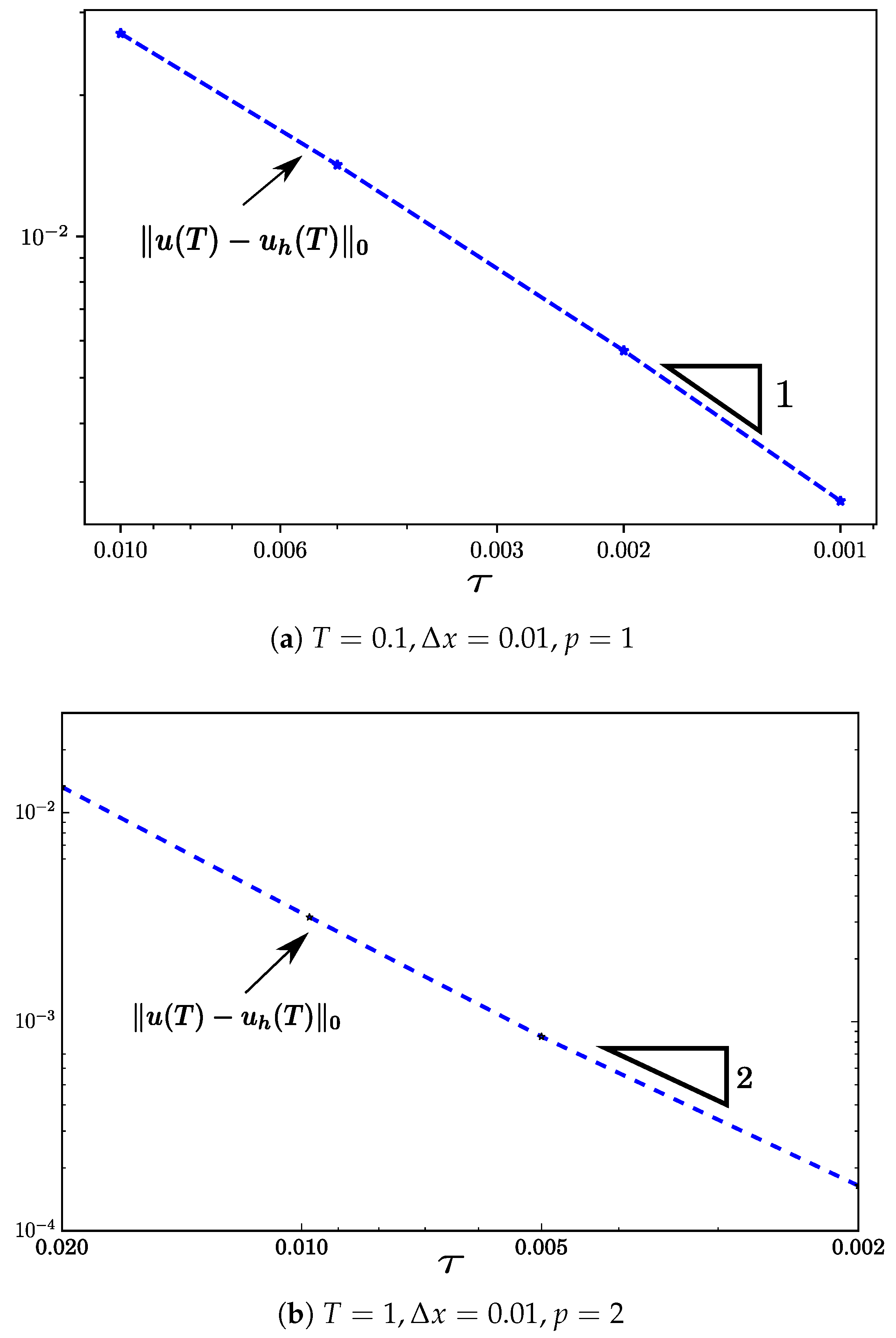
5.1. Heat Equation (2D)

We start the method’s performance analysis by solving the 2D heat equation while refining the spatial domain uniformly. Although this case does not present any particular challenge to classical methods, it is a standard benchmark problem to test space and time convergences of parabolic problems.

Let the domain $\mathsf{\Omega }$ be ${[0,1]}^2$; we consider the problem:

$$\begin{array}{cccc}\hfill {\partial }_{t}u-\Delta u& =& f\hfill & \mathrm{in}\mathsf{\Omega }\times (0,T],\hfill \\ \hfill u& =& 0\hfill & \mathrm{on}{\mathsf{\Gamma }}_D\times (0,T],\hfill \\ \hfill u(·,t=0)& =& u_0\hfill & \mathrm{in}\mathsf{\Omega },\hfill \end{array}$$

(38)

with the initial condition:

$$u_0=sin\left(\pi x\right)sin\left(\pi y\right),$$

and the source term f that satisfies the exact solution:

$$u((x,y),t)=exp(-{\pi }^{2}t)sin\left(\pi x\right)sin\left(\pi y\right).$$

To formulate the fully discrete problem, we combine the SIP billinear form (for $\kappa =1$) with the BDF1/BDF2 time marching scheme. We show the convergence plots for linear and quadratic polynomials in space (Figure 2 and Figure 3) and time (Figure 4). To perform the spatial convergence test, we compute the errors $\Vert u-u_h{\Vert }_{\tau }$ (in black), $\Vert u-{\theta }_h{\Vert }_{\tau }$ (in blue), $\Vert {\theta }_h-u_h{\Vert }_{\tau }$ (in green) and $\Vert {\epsilon }_h{\Vert }_{\tau }$ (in red) for different mesh sizes ($\Delta x$). We denote $\Delta x$ equal to $h_K$ for uniform meshes. To perform the time convergence, we show $\Vert u-u_h{\Vert }_0$ varying with the time step $\tau$ for $\Delta x=0.01$. As a result, we recover space optimality for the continuous approximation (from dG formulation) and the first- and second-order time convergence for BDF1 and BDF2, respectively. We show that the saturation assumption in [30] holds in our formulation (i.e., $\Vert u\left(T\right)-{\theta }_h{\left(T\right)\Vert }_{\tau }\lesssim {\Vert u\left(T\right)-u_h\left(T\right)\Vert }_{\tau }$) and the residual representation is efficient until the error dominates (i.e., $\Vert {\epsilon }_h{\Vert }_{\tau }\lesssim {\Vert u\left(T\right)-u_h\left(T\right)\Vert }_{\tau }$ in [30]). To illustrate, Figure 3b shows that for $p=2$ and high DoF, the temporal error is no longer negligible to the spatial error; however, the error estimator continues decaying since it does not consider the temporal error contribution. We will seek to prove these properties in future work.

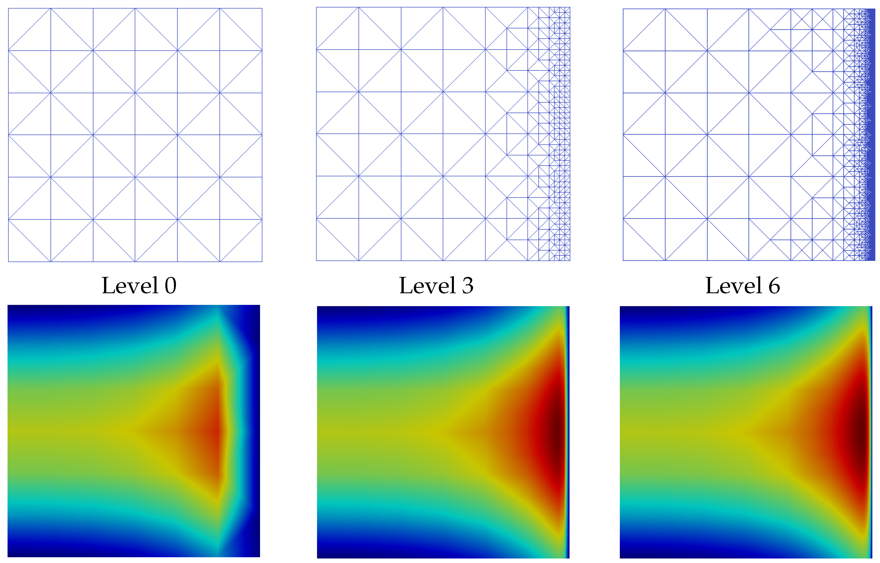
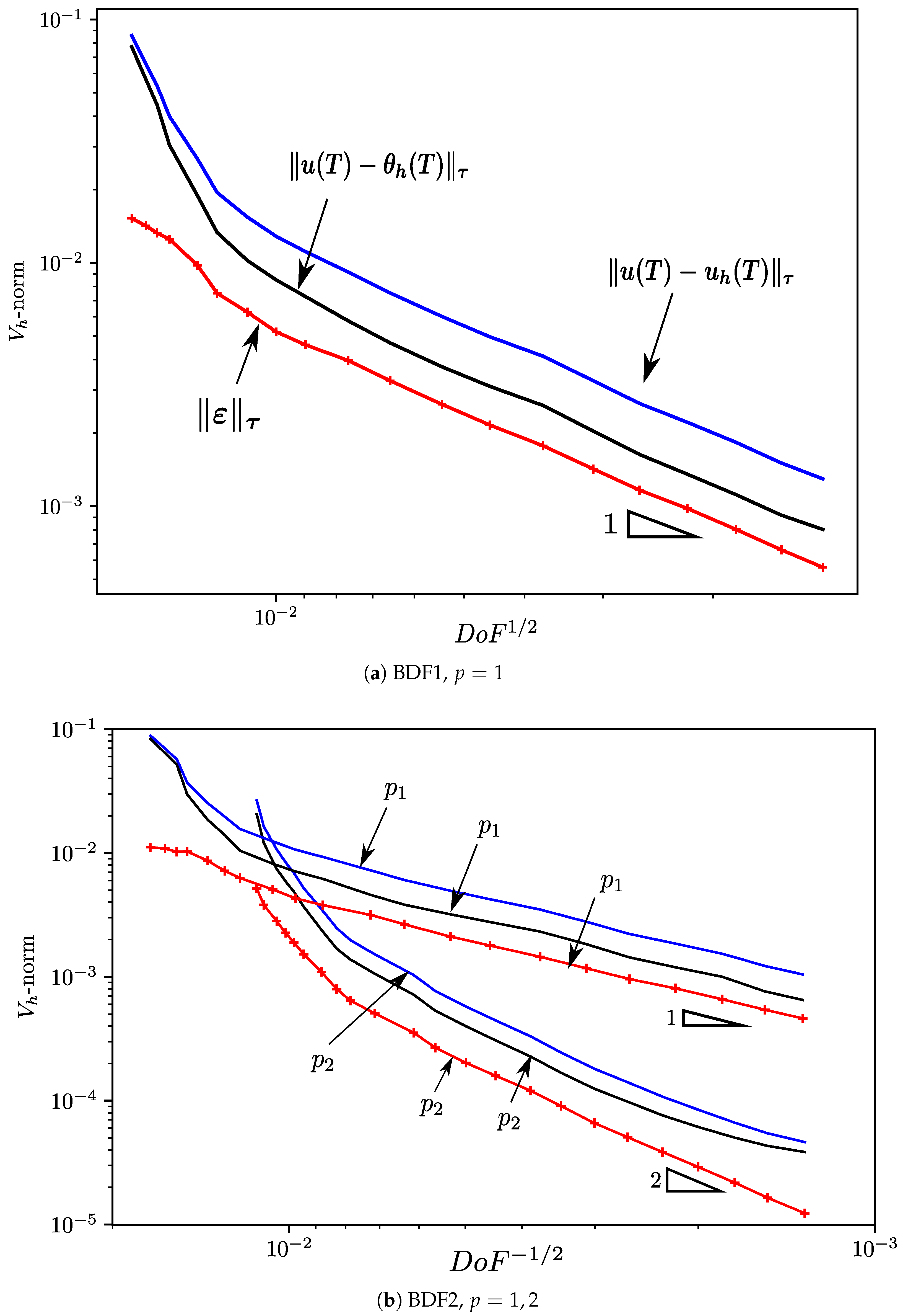
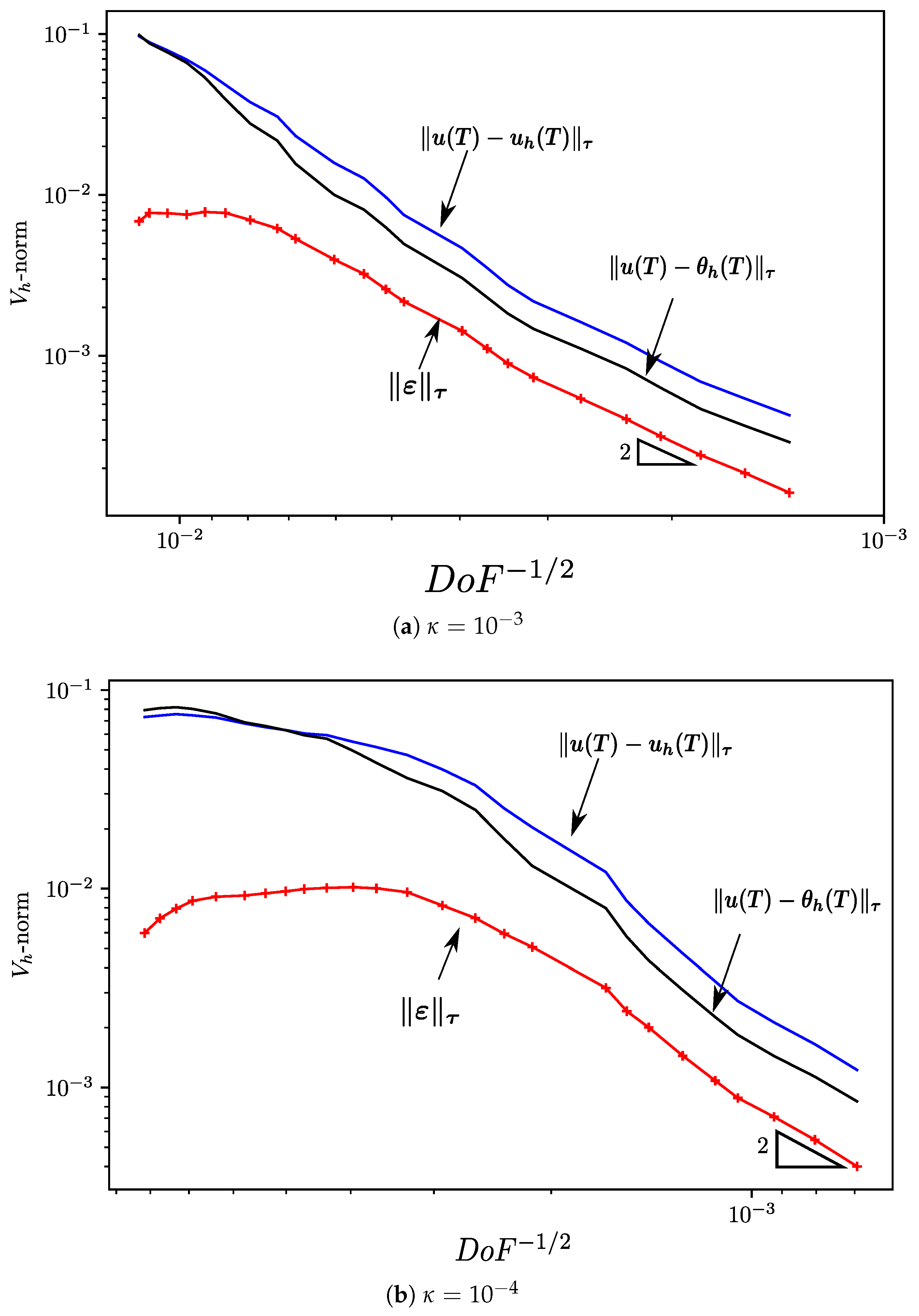
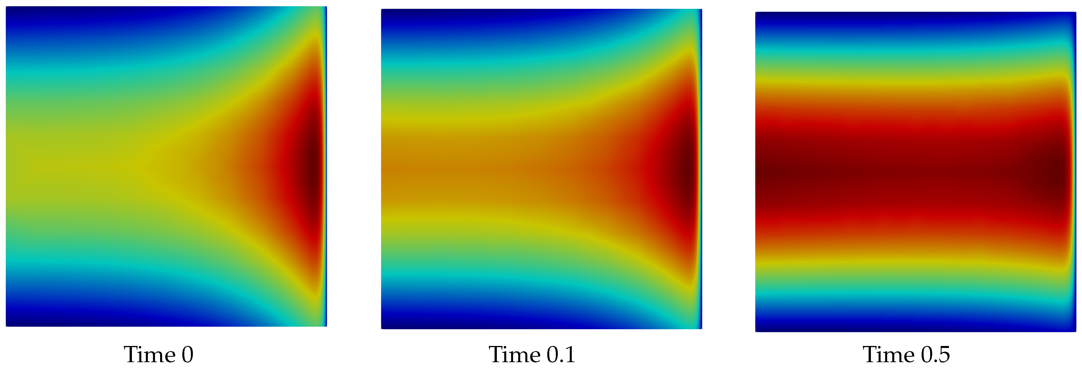
5.2. Advection–Diffusion Problem

We complement the spatial convergence study of the previous example, using adaptive refinement for the unsteady advection–dominated Eriksson–Johnson problem. Let the domain $\mathsf{\Omega }$ be $[0,1]\times [-0.5,0.5]$; we consider the exact solution

$$u((x,y),t)=exp(-lt)[exp\left({\lambda }_{1}x\right)-exp\left({\lambda }_{2}x\right)]+cos\left(\pi y\right)\frac{exp\left(s_{1}x\right)-exp\left(r_{1}x\right)}{exp(-s1)-exp(-r_1)},$$

for $f=0$ and $l=2$, ${\lambda }_{1,2}=\frac{-1\pm \sqrt{1-4\kappa l}}{-2\kappa }$, $r_1=\frac{1+\sqrt{1+4{\kappa }^2{\pi }^2}}{2\kappa }$ and $s_1=\frac{1-\sqrt{1+4{\kappa }^2{\pi }^2}}{2\kappa }$. Here, we set $\beta =[1,0]$ and $\mu =0$ for different diffusion coefficient values. Based on the exact solution, we apply Neumann boundary conditions at $x=-1$ and $t=0$; meanwhile, we impose Dirichlet boundary conditions at $x=0$, $y=-0.5$ and $y=0.5$ at time $t=0$.

The problem’s main challenge is capturing the boundary layer, especially for high Péclet numbers. Figure 5 shows how the error estimator drives spatial adaptivity to smooth the regions with sharp gradients in each time step. Figure 6 shows the errors $\Vert u-u_h{\Vert }_{\tau }$, $\Vert u-{\theta }_h{\Vert }_{\tau }$ and $\Vert {\epsilon }_h{\Vert }_{\tau }$ versus the square of total degrees of freedom ($Do{F}^{1/2}$) (i.e., $dim\left(U_h\right)+dim\left(V_h\right)$ ); these plots verify the optimal spatial convergence in the fully discrete energy norm using BDF1 and BDF2 time integrators for linear and quadratic polynomial trial functions at $T=0.1$ and $\tau =0.005$. In Figure 7, we verify our method’s convergence for higher Péclet numbers by setting the diffusivity in ${10}^{-3}$ and ${10}^{-4}$. Figure 8 shows the evolution of our transient solution to the analytical steady-state Eriksson–Johnson. Similarly to the uniform refinement case, we preserve the efficiency of the residual representative and the saturation assumptions as stated for the adaptive steady state case.

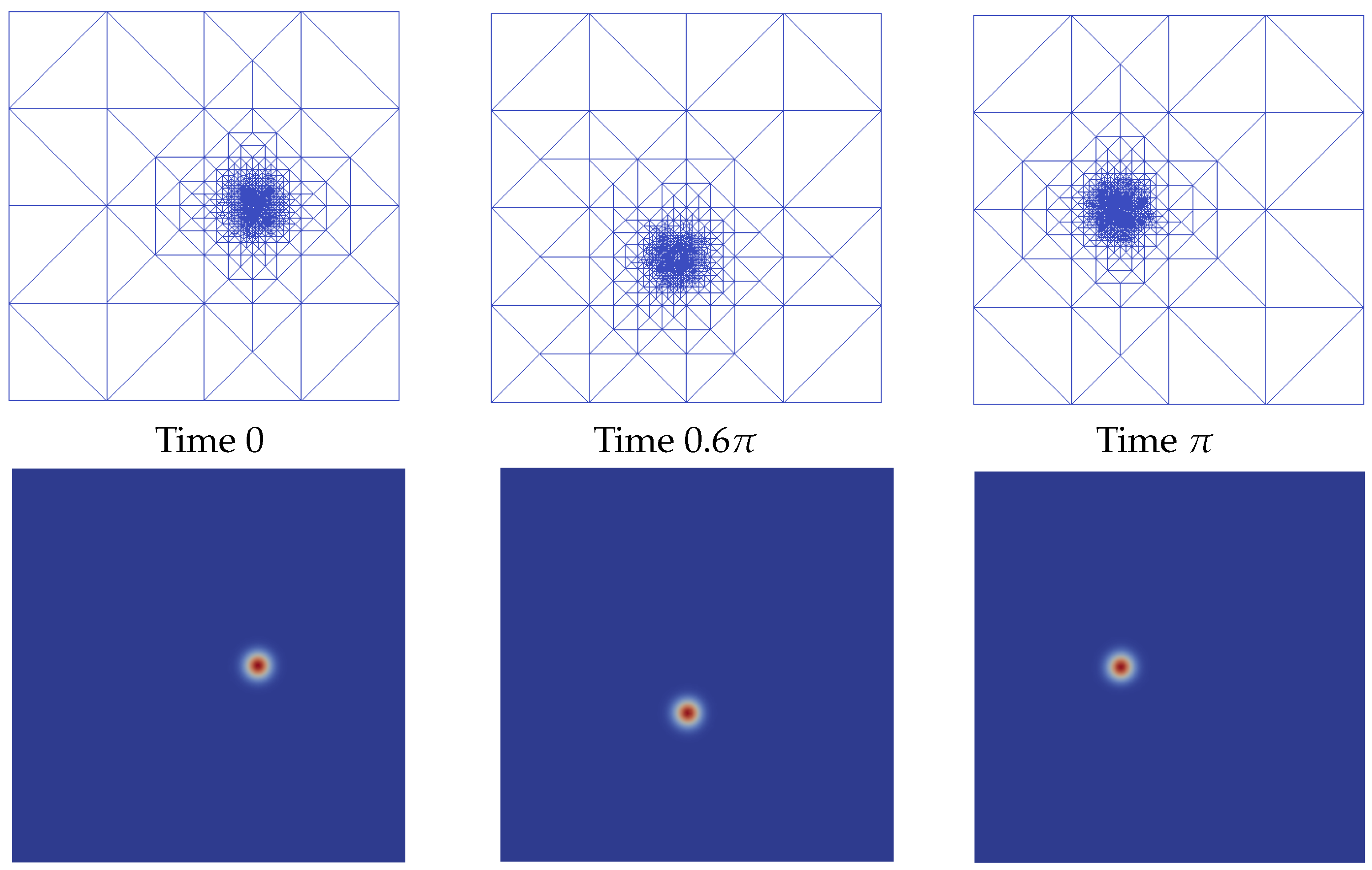
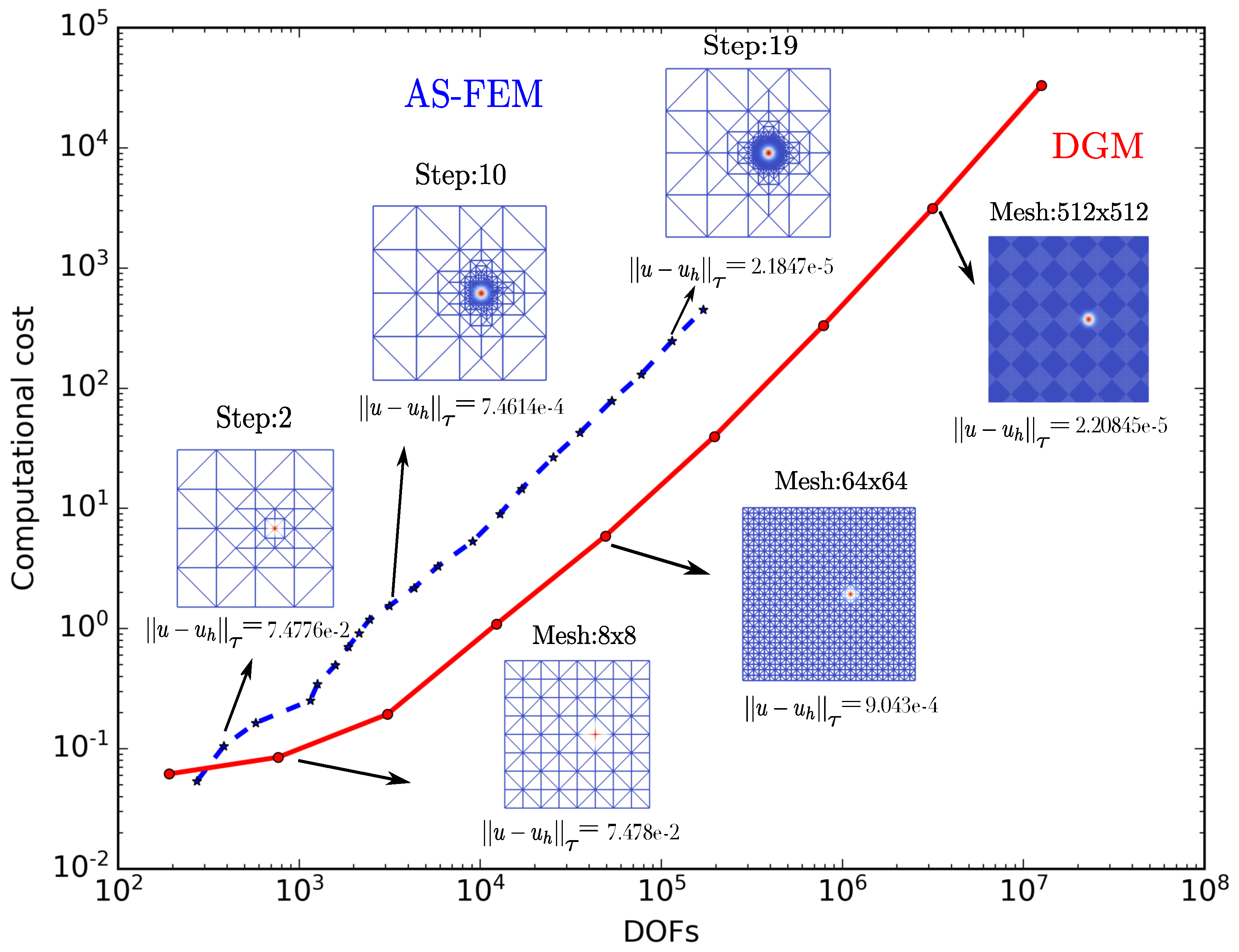
5.3. Rotating Flow Transporting a Gaussian Profile

In this example, we analyze the performance of our method in a convective transport problem with a localized disturbance. Thus, we test the adaptive algorithm in the case where the region of interest moves within the domain as time passes. We study the solution of a 2D convection–diffusion transport by a rotatory flow of a Gaussian profile. We set $\mathsf{\Omega }={[-2,2]}^2$, $T=\pi$, $\beta =[y,-x]$, $\kappa ={10}^{-5}$, $\mu =0$ and $f=0$. The initial condition is

$$u_0=exp(-64{(x-0.5)}^2)exp(-64y^2),$$

we impose Dirichlet boundary conditions from the exact solution:

$$u((x,y),t)={\displaystyle \frac{1}{1+256\kappa t}}exp\left(-{\displaystyle \frac{64{(x-0.5cos\left(t\right))}^2}{1+256\kappa t}}\right)exp\left(-{\displaystyle \frac{64{(y+0.5sin\left(t\right))}^2}{1+256\kappa t}}\right).$$

Figure 9 shows the profiles of the solutions and the corresponding adaptively refined meshes at different time steps. These results demonstrate the continuous solution stability and consistency with the physical phenomena, even for low diffusivities. Moreover, the mesh nodes concentrate where the solution varies largely, showing the robustness of the error estimator and the efficiency of the marking strategy when adding new degrees of freedom. Regarding computational cost, our stabilized finite element formulation using adaptivity is competitive with the dG methodology using uniform refinement. Solving the saddle point formulation requires an extra cost due to the additional degrees of freedom. However, adaptivity compensates for the excess due to the solution’s stability in coarse meshes and the robustness of the error estimator. Figure 10 shows a comparison between the total computational cost required to obtain a solution with the adaptive stabilized method (blue line) and the computational cost using a regular mesh in the dG method (red line). Besides, the figure shows that the adaptivity can reduce the computational cost by up to one order of magnitude to get a resolution of 1 × 10${}^{-5}$ in the energy norm.

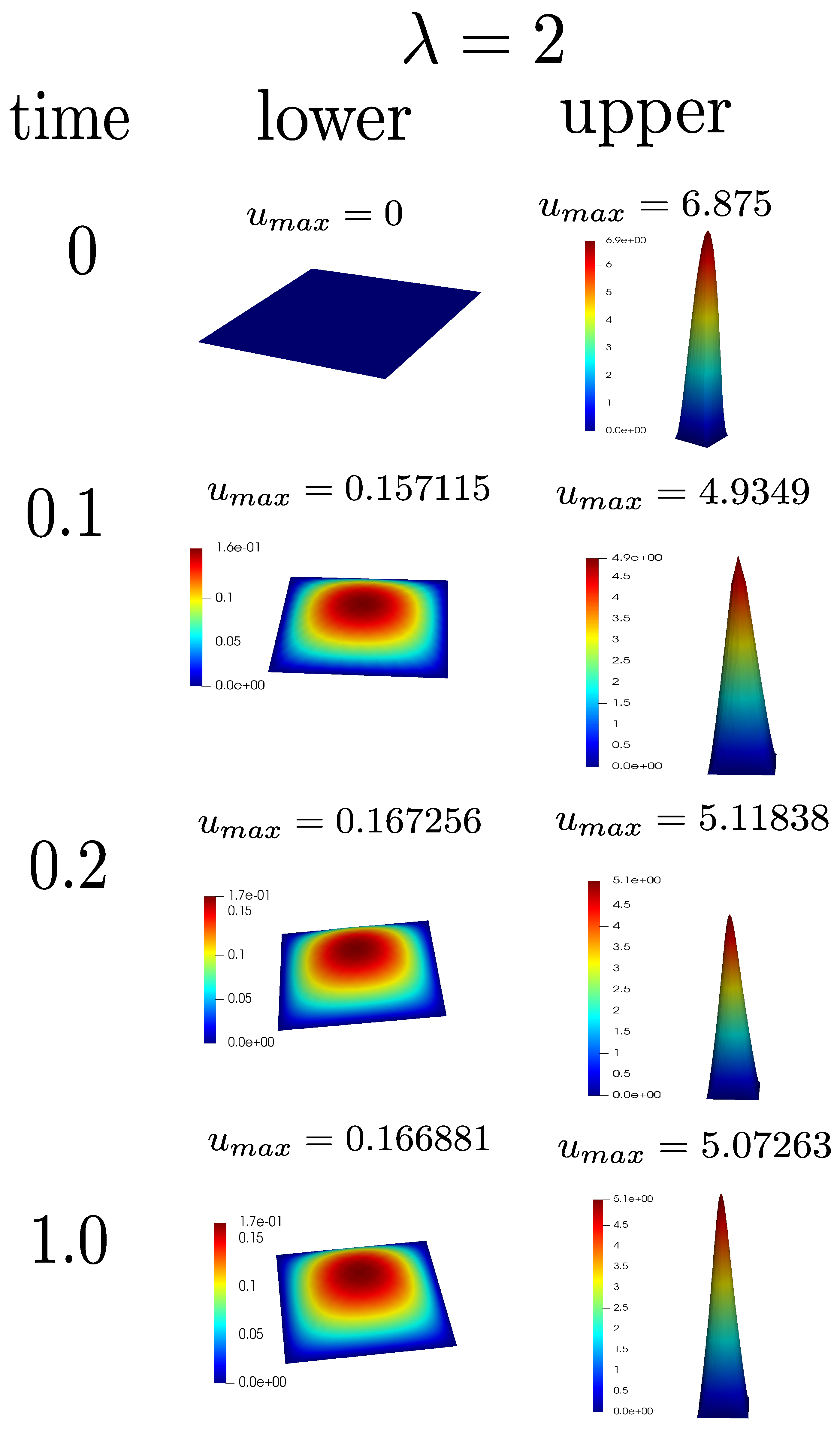
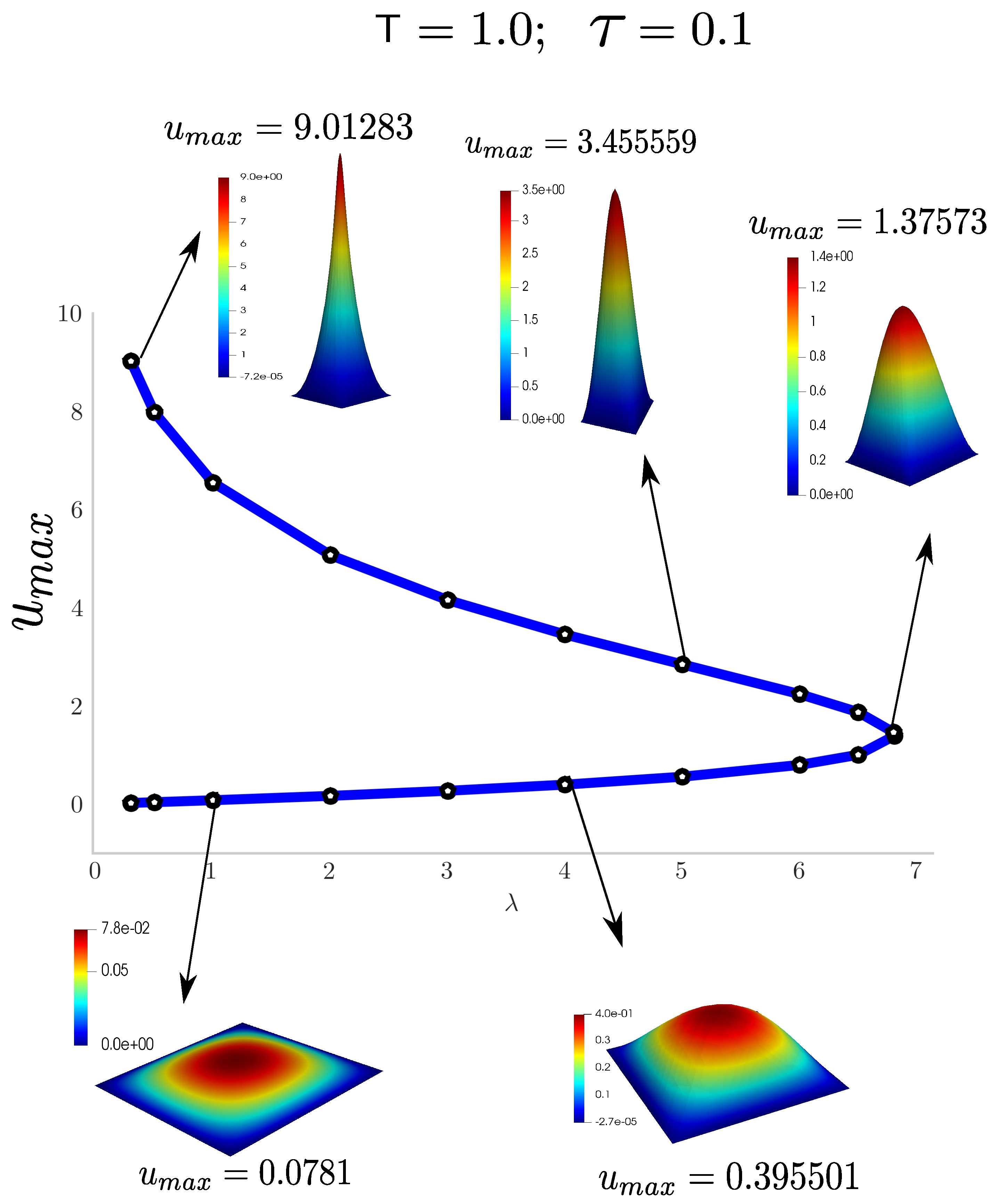
5.4. Unsteady Bratu Equation: Non-Linear Diffusion-Reaction Equation

We conclude the method’s performance analysis by studying the solution of a nonlinear diffusion-reaction equation. Let $\lambda$ be a positive real constant and $\mathsf{\Omega }={[0,1]}^2$; we solve the unsteady version of Bratu’s problem in the following form:

$$\left\{\begin{array}{c}\mathrm{Find}u\mathrm{such}\mathrm{that},\mathrm{for}T>0,\hfill \\ \begin{array}{ccc}\hfill {\partial }_{t}u=\Delta u+\lambda \exp \left(u\right)& & \mathrm{in}\mathsf{\Omega }\times (0,T],\hfill \\ \hfill u=0& & \mathrm{on}\mathsf{\Gamma }\times (0,T],\hfill \\ \hfill u(·,t=0)=u_0\left(x\right)& & \mathrm{in}\mathsf{\Omega },\hfill \end{array}\hfill \end{array}\right.$$

(39)

The two-dimensional steady version of (39) has a branched solution for $\lambda <{\lambda }_c$ (lower and upper branches) and a unique solution when $\lambda ={\lambda }_c$, with ${\lambda }_c\approx 6.8081$ as a critical point. The problem’s main challenges are the lack of stable solutions in the upper branch and close to the critical point ${\lambda }_c$, leading to classical techniques converging only to the stable lower branch. We test our method’s robustness, accuracy and performance in this transient bifurcation problem; we compare the solutions obtained in (39) when $t\to \infty ,$ with the 2D steady Bratu’s approach obtained in [33]. We formulate the space semi-discretization of (39) as follows:

$$\left\{\begin{array}{c}\mathrm{Find}{\theta }_h\in V_h,\mathrm{such}\mathrm{that}:\hfill \\ \begin{array}{c}{({\partial }_t{\theta }_h,v_h)}_0+{\eta }_h({\theta }_h;v_h)={\ell }_h\left(v_h\right),\forall v_h\in V_h,\hfill \end{array}\hfill \end{array}\right.$$

(40)

where ${\eta }_h(u_h;v_h)$ denotes the nonlinear form, including the SIP formulation in (7) with a non-linear reactive contribution. We define it as:

$$\begin{array}{cc}\hfill {\displaystyle {\eta }_h(u_h;v_h):}& =\sum _{K\in \mathfrak{T}}{({\nabla }_h{u}_h·{\nabla }_h{v}_h)}_K-\sum _{K\in {\mathcal{S}}_h}{(\lambda exp\left(u_h\right),v_h)}_K\hfill \\ \hfill & -\sum _{F\in {\mathcal{S}}_h^{\partial }}\left({(\left\{{\nabla }_h{u}_h\right\}·{\mathbf{n}}_F,\left[\left[v_h\right]\right])}_F+{(\left[\left[u_h\right]\right],\left\{{\nabla }_h{v}_h\right\}·{\mathbf{n}}_F)}_F-n_e\kappa {(\left[\left[u_h\right]\right],\left[\left[v_h\right]\right])}_F\right).\hfill \end{array}$$

(41)

For BDF1 time marching, we define the discrete-time nonlinear form as:

$$\begin{array}{ccc}{\eta }_{h,\tau }(u_h;v_h)\hfill & :=\hfill & {(u_h,v_h)}_K+\tau {\eta }_h(u_h;v_h).\hfill \end{array}$$

(42)

Thus, the full-discrete formulation for problem (39) is:

$$\left\{\begin{array}{c}\mathrm{Given}{\theta }_h^n,\mathrm{find}{\theta }_h^{n+1}\in V_h\mathrm{such}\mathrm{that}:\hfill \\ {\eta }_{h,\tau }({\theta }_h^{n+1};v_h)={(l_h^{\mathrm{dG}},v_h)}_0\forall v_h\in V_h,\hfill \end{array}\right.$$

(43)

with $l_h^{\mathrm{dG}}:={\theta }_h^n+\tau {\ell }_h^{n+1}.$ We use a Newton–Raphson iteration scheme combined with the residual minimization strategy described in Section 4 to solve (43). We seek a solution at every Newton step increment $w_h$ for each time step $n+1$ by using the linearized form:

$$\begin{array}{c}\hfill {\displaystyle {\eta }_{h,\tau }^{\prime }(u_h;w_h,v_h):={(w_h,v_h)}_K+\tau (\sum _{K\in \mathfrak{T}}{({\nabla }_h{w}_h·{\nabla }_h{v}_h)}_K-\sum _{K\in {\mathcal{S}}_h}{(\lambda exp\left(u_h\right)w_h,v_h)}_K}\\ \hfill -\sum _{F\in {\mathcal{S}}_h}\left({(\left\{{\nabla }_h{w}_h\right\}·{\mathbf{n}}_F,\left[\left[v_h\right]\right])}_F+{(\left[\left[w_h\right]\right],\left\{{\nabla }_h{v}_h\right\}·{\mathbf{n}}_F)}_F-n_e\kappa {(\left[\left[w_h\right]\right],\left[\left[v_h\right]\right])}_F\right))\end{array}$$

(44)

Since (44) takes the form of a diffusion-reaction problem, we use a time-step dependent norm (22), with the SIP contribution to the $V_h-$norm, to minimize the discrete residual of the linearized system. The norm ${\Vert ·\Vert }_{\tau }$ is enforced with an $L_2$ contribution to measure the nonlinear reactive term. Starting with an initial guess $({\epsilon }_{h,0}^{n+1},u_{h,0}^{n+1})$ and given $({\epsilon }_{h,i}^{n+1},u_{h,i}^{n+1})$, we find:

$$\left\{\begin{array}{c}(\delta {\epsilon }_h^{n+1},\delta u_h^{n+1})\in V_h\times U_h,\mathrm{such}\mathrm{that}:\forall (z_h,v_h)\in V_h,\times U_h\hfill \\ \begin{array}{cc}\hfill {(\delta {\epsilon }_h^{n+1},v_h)}_{\tau }+{\eta }_{h,\tau }^{\prime }(u_{h,i}^{n+1};\delta u_h^{n+1},v_h)& ={(l_h,v_h)}_0-{({\epsilon }_{h,i}^{n+1},v_h)}_{\tau }-{\eta }_{h,\tau }(u_{h,i}^{n+1};v_h)\hfill \\ \hfill {\eta }_{h,\tau }^{\prime }(u_{h,i}^{n+1};z_h,\delta {\epsilon }_h^{n+1})& =-{\eta }_{h,\tau }^{\prime }(u_{h,i}^{n+1};z_h,{\epsilon }_{h,i}^{n+1})\hfill \end{array}\hfill \end{array}\right.$$

(45)

$u_{h,i}^{n+1}$ and ${\epsilon }_{h,i}^{n+1}$ are updated at every i-th increment as follows:

$$u_{h,i+1}^{n+1}=u_{h,i}^{n+1}+k\delta u_h^{n+1},{\epsilon }_{h,i+1}^{n+1}={\epsilon }_{h,i}^{n+1}+k\delta {\epsilon }_h^{n+1},$$

where k denotes a relaxation parameter from the Damped Newton’s method [46], and it is detailed to our formulation’s context in [33]. For the time step $n=1$, we set the initial guess $({\epsilon }_{h,0}^{n+1},u_{h,0}^{n+1})=(0,u_{\mathrm{IG}})$, where $u_{\mathrm{IG}}$ varies depending on the solution branch we want to capture. Here, we assume $u_{\mathrm{IG}}$ equal to the initial solution (i.e., $u_{\mathrm{IG}}=u_0$) with $u_0=0$ for the stable lower branch and $u_0=u_{\mathrm{up}}$ for the upper branch. Since the lower branch is stable, many different initial guesses converge to it; however, we only use one option. The unstable upper branch is more restrictive; therefore, we follow [47] and use:

$$u_{\mathrm{up}}(x,y)=\frac{50(2+\lambda )}{\lambda }(x-x^2)(y-y^2).$$

Figure 11 and Figure 12 show the two branch solutions obtained for a time step increment $\tau =0.1$ with an initial mesh of 4 × 4 elements and a final time $T=1.0$. Figure 11 shows a time sequence for lower and upper solutions from $t=0$ to $t=T$ at $\lambda =2$. Figure 12 shows the classical bifurcation diagram for Bratu’s problem evaluating the maximum value $u_{\max }$ at the time T for different $\lambda$ values from 0 to ${\lambda }_c$. At this time, we guarantee a convergent solution over time to approach the steady state of this problem. We demonstrate the robustness of our approach and the efficient refinement strategy to capture all stable and unstable branches, even close to the critical point (${\lambda }_c$). We test the accuracy of the results by successfully validating our bifurcation map at time T with results obtained from different authors at the steady state [31,47].

6. Discussion

This paper proposes an adaptive-stabilized finite element method based on residual minimization for unsteady advection–diffusion–reaction problems using the method of lines. The method provides a stable solution and a robust error representation to guide adaptivity at every discrete time. We demonstrate the method’s performance for challenging linear and nonlinear problems with optimal spatial and temporal convergence and the efficiency of the adaptive refinement strategy to capture sharp inner and boundary layers. We present evidence that the adaptive refinement process could overcome the required computational cost to solve the saddle-point problem compared to the uniformly refined schemas on discontinuous Galerkin approximation. Other time-marching approaches, including explicit time-marching schemas with time adaptivity and space–time formulation, will be described in future publications.

References

1. Brooks, A.N.; Hughes, T.J. Streamline upwind/Petrov–Galerkin formulations for convection dominated flows with particular emphasis on the incompressible Navier–Stokes equations. Comput. Methods Appl. Mech. Eng. 1982, 32, 199–259. [Google Scholar] [CrossRef]
2. Hughes, T.J.R.; Franca, L.P.; Hulbert, G.M. A new finite element formulation for computational fluid dynamics: VIII. The Galerkin/Least-Squares method for advection–diffusive equations. Comput. Methods Appl. Mech. Eng. 1989, 73, 173–189. [Google Scholar] [CrossRef]
3. Hughes, T.J.; Feijóo, G.R.; Mazzei, L.; Quincy, J.B. The variational multiscale method—A paradigm for computational mechanics. Comput. Methods Appl. Mech. Eng. 1998, 166, 3–24. [Google Scholar] [CrossRef]
4. Hughes, T.J.R.; Scovazzi, G.; Franca, L.P. Multiscale and Stabilized Methods. In Encyclopedia of Computational Mechanics, 2nd ed.; American Cancer Society: Kennesaw, GA, USA, 2017; pp. 1–64. [Google Scholar]
5. Bazilevs, Y.; Calo, V.; Cottrell, J.; Hughes, T.; Reali, A.; Scovazzi, G. Variational multiscale residual-based turbulence modeling for large eddy simulation of incompressible flows. Comput. Methods Appl. Mech. Eng. 2007, 197, 173–201. [Google Scholar] [CrossRef]
6. Bazilevs, Y.; Michler, C.; Calo, V.; Hughes, T. Isogeometric variational multiscale modeling of wall-bounded turbulent flows with weakly enforced boundary conditions on unstretched meshes. Comput. Methods Appl. Mech. Eng. 2010, 199, 780–790. [Google Scholar] [CrossRef]
7. Chang, K.; Hughes, T.; Calo, V. Isogeometric variational multiscale large-eddy simulation of fully-developed turbulent flow over a wavy wall. Comput. Fluids 2012, 68, 94–104. [Google Scholar] [CrossRef]
8. Ghaffari Motlagh, Y.; Ahn, H.T.; Hughes, T.J.; Calo, V.M. Simulation of laminar and turbulent concentric pipe flows with the isogeometric variational multiscale method. Comput. Fluids 2013, 71, 146–155. [Google Scholar] [CrossRef]
9. Arnold, D.N.; Brezzi, F.; Cockburn, B.; Donatella Marini, L. Unified analysis of discontinuous Galerkin methods for elliptic problems. SIAM J. Numer. Anal. 2001, 39, 1749–1779. [Google Scholar] [CrossRef]
10. Burman, E.; Hansbo, P. Edge stabilization for Galerkin approximations of convection-diffusion-reaction problems. Comput. Methods Appl. Mech. Eng. 2004, 193, 1437–1453. [Google Scholar] [CrossRef] [Green Version]
11. Brezzi, F.; Marini, L.D.; Süli, E. Discontinuous Galerkin methods for first-order hyperbolic problems. Math. Model. Methods Appl. Sci. 2004, 14, 1893–1903. [Google Scholar] [CrossRef]
12. Ayuso, B.; Marini, L.D. Discontinuous Galerkin methods for advection–diffusion–reaction problems. SIAM J. Numer. Anal. 2009, 47, 1391–1420. [Google Scholar] [CrossRef]
13. Cockburn, B.; Karniadakis, G.E.; Shu, C.W. Discontinuous Galerkin Methods: Theory, Computation and Applications; Springer Science & Business Media: Berlin/Heidelberg, Germany, 2012; Volume 11. [Google Scholar]
14. Demwkowicz, L.; Gopalakrishnan, J. Analysis of the DPG Method for the Poisson Equation. SIAM J. Numer. Anal. 2011, 49, 1788–1809. [Google Scholar] [CrossRef] [Green Version]
15. Zitelli, J.; Muga, I.; Demkowicz, L.; Gopalakrishnan, J.; Pardo, D.; Calo, V. A class of discontinuous Petrov–Galerkin methods. Part IV: The optimal test norm and time-harmonic wave propagation in 1D. J. Comput. Phys. 2011, 230, 2406–2432. [Google Scholar] [CrossRef] [Green Version]
16. Niemi, A.H.; Collier, N.O.; Calo, V.M. Automatically stable discontinuous Petrov–Galerkin methods for stationary transport problems: Quasi-optimal test space norm. Comput. Math. Appl. 2013, 66, 2096–2113. [Google Scholar] [CrossRef]
17. Cockburn, B.; Shu, C.W. The local discontinuous Galerkin method for time-dependent convection–diffusion systems. SIAM J. Numer. Anal. 1998, 35, 2440–2463. [Google Scholar] [CrossRef]
18. Borker, R.; Farhat, C.; Tezaur, R. A high-order discontinuous Galerkin method for unsteady advection–diffusion problems. J. Comput. Phys. 2017, 332, 520–537. [Google Scholar] [CrossRef]
19. Rivière, B. Discontinuous Galerkin Methods for Solving Elliptic and Parabolic Equations: Theory and Implementation; SIAM: Philadelphia, PA, USA, 2008. [Google Scholar]
20. Di Pietro, D.A.; Ern, A. Mathematical Aspects of Discontinuous Galerkin Methods; Springer Science & Business Media: Berlin/Heidelberg, Germany, 2011; Volume 69. [Google Scholar]
21. Demkowicz, L.; Gopalakrishnan, J. A class of discontinuous Petrov–Galerkin methods. Part I: The transport equation. Comput. Methods Appl. Mech. Eng. 2010, 199, 1558–1572. [Google Scholar] [CrossRef] [Green Version]
22. Führer, T.; Heuer, N.; Karkulik, M. Analysis of backward Euler primal DPG methods. Comput. Methods Appl. Math. 2021, 21, 811–826. [Google Scholar] [CrossRef]
23. Barrenechea, G.R.; Brezzi, F.; Cangiani, A.; Georgoulis, E.H. Building Bridges: Connections and Challenges in Modern Approaches to Numerical Partial Differential Equations; Springer: Berlin/Heidelberg, Germany, 2016. [Google Scholar]
24. Roberts, N.V.; Henneking, S. Time-stepping DPG formulations for the heat equation. Comput. Math. Appl. 2020, 95, 242–255. [Google Scholar] [CrossRef]
25. Ern, A.; Vohralík, M. A posteriori error estimation based on potential and flux reconstruction for the heat equation. SIAM J. Numer. Anal. 2010, 48, 198–223. [Google Scholar] [CrossRef]
26. Zhu, L.; Schötzau, D. A robust a posteriori error estimate for hp-adaptive DG methods for convection–diffusion equations. IMA J. Numer. Anal. 2010, 31, 971–1005. [Google Scholar] [CrossRef] [Green Version]
27. Ern, A.; Proft, J. A posteriori discontinuous Galerkin error estimates for transient convection-diffusion equations. Appl. Math. Lett. 2005, 18, 833–841. [Google Scholar] [CrossRef] [Green Version]
28. Araya, R.; Venegas, P. An a posteriori error estimator for an unsteady advection-diffusion- reaction problem. Comput. Math. Appl. 2014, 66, 2456–2476. [Google Scholar] [CrossRef]
29. Cangiani, A.; Georgoulis, E.H.; Metcalfe, S. Adaptive discontinuous Galerkin methods for nonstationary convection-diffusion problems. IMA J. Numer. Anal. 2014, 34, 1578–1597. [Google Scholar] [CrossRef] [Green Version]
30. Calo, V.M.; Ern, A.; Muga, I.; Rojas, S. An adaptive stabilized conforming finite element method via residual minimization on dual discontinuous Galerkin norms. Comput. Methods Appl. Mech. Eng. 2020, 363, 112891. [Google Scholar] [CrossRef] [Green Version]
31. Cier, R.J.; Rojas, S.; Calo, V.M. Automatically adaptive, stabilized finite element method via residual minimization for heterogeneous, anisotropic advection–diffusion–reaction problems. Comput. Methods Appl. Mech. Eng. 2021, 385, 114027. [Google Scholar] [CrossRef]
32. Calo, V.; Łoś, M.; Deng, Q.; Muga, I.; Paszyński, M. Isogeometric Residual Minimization Method (iGRM) with direction splitting preconditioner for stationary advection-dominated diffusion problems. Comput. Methods Appl. Mech. Eng. 2021, 373, 113214. [Google Scholar] [CrossRef]
33. Cier, R.J.; Rojas, S.; Calo, V.M. A nonlinear weak constraint enforcement method for advection-dominated diffusion problems. Mech. Res. Commun. 2021, 112, 103602. [Google Scholar] [CrossRef]
34. Rojas, S.; Pardo, D.; Behnoudfar, P.; Calo, V.M. Goal-oriented adaptivity for a conforming residual minimization method in a dual discontinuous Galerkin norm. Comput. Methods Appl. Mech. Eng. 2021, 377, 113686. [Google Scholar] [CrossRef]
35. Kyburg, F.E.; Rojas, S.; Calo, V.M. Incompressible flow modeling using an adaptive stabilized finite element method based on residual minimization. Int. J. Numer. Methods Eng. 2022, 123, 1717–1735. [Google Scholar] [CrossRef]
36. Łoś, M.; Rojas, S.; Paszyński, M.; Muga, I.; Calo, V.M. DGIRM: Discontinuous Galerkin based isogeometric residual minimization for the Stokes problem. J. Comput. Sci. 2021, 50, 101306. [Google Scholar] [CrossRef]
37. Poulet, T.; Giraldo, J.F.; Ramanaidou, E.; Piechocka, A.; Calo, V.M. Paleo-stratigraphic permeability anisotropy controls supergene mimetic martite goethite deposits. Basin Res. 2022. [Google Scholar] [CrossRef]
38. Labanda, N.A.; Espath, L.; Calo, V.M. A spatio-temporal adaptive phase-field fracture method. Comput. Methods Appl. Mech. Eng. 2022, 392, 114675. [Google Scholar] [CrossRef]
39. Bramble, J.H.; Thomée, V. Semidiscrete least-squares methods for a parabolic boundary value problem. Math. Comput. 1972, 26, 633–648. [Google Scholar]
40. Becker, J. A second order backward difference method with variable steps for a parabolic problem. BIT Numer. Math. 1998, 38, 644–662. [Google Scholar] [CrossRef]
41. Crouzeix, M.; Lisbona, F. The convergence of variable-stepsize, variable-formula, multistep methods. SIAM J. Numer. Anal. 1984, 21, 512–534. [Google Scholar] [CrossRef]
42. Ern, A.; Stephansen, A.F.; Zunino, P. A discontinuous Galerkin method with weighted averages for advection–diffusion equations with locally small and anisotropic diffusivity. IMA J. Numer. Anal. 2009, 29, 235–256. [Google Scholar] [CrossRef]
43. Dörfler, W. A convergent adaptive algorithm for Poisson’s equation. SIAM J. Numer. Anal. 1996, 33, 1106–1124. [Google Scholar] [CrossRef]
44. Bank, R.E.; Welfert, B.D.; Yserentant, H. A class of iterative methods for solving saddle point problems. Numer. Math. 1989, 56, 645–666. [Google Scholar] [CrossRef]
45. Alnæs, M.; Blechta, J.; Hake, J.; Johansson, A.; Kehlet, B.; Logg, A.; Richardson, C.; Ring, J.; Rognes, M.E.; Wells, G.N. The FEniCS project version 1.5. Arch. Numer. Softw. 2015, 3. [Google Scholar] [CrossRef]
46. Bank, R.E.; Rose, D.J. Global approximate Newton methods. Numer. Math. 1981, 37, 279–295. [Google Scholar] [CrossRef]
47. Hajipour, M.; Jajarmi, A.; Baleanu, D. On the accurate discretization of a highly nonlinear boundary value problem. Numer. Algorithms 2018, 79, 679–695. [Google Scholar] [CrossRef]
Figure 1. Notation of the element interface.
Mca 28 00007 g001
Figure 2. BDF1 spatial convergence using fixed time step and uniform meshes.
Mca 28 00007 g002
Figure 3. BDF2 spatial convergence using fixed time step and uniform meshes.
Mca 28 00007 g003aMca 28 00007 g003b
Figure 4. Time convergence for BDF1 and BDF2 time integrators using a fixed mesh.
Mca 28 00007 g004
Figure 5. Mesh refinement τ = 0.005 , T = 0.1 , p = 1 .
Mca 28 00007 g005
Figure 6. Spatial convergence for adaptive refinement (BDF1 & BDF2: κ = 10 2 , T = 0.1 , τ = 0.005 ).
Mca 28 00007 g006
Figure 7. Spatial convergence for adaptive refinement using BDF2. p = 2 , T = 0.1 , τ = 0.005 .
Mca 28 00007 g007
Figure 8. Solution convergence to the steady Eriksson–Johnson solution.
Mca 28 00007 g008
Figure 9. Time evolution p = 1 ( T = π , τ = π / 512 ).
Mca 28 00007 g009
Figure 10. Computational cost [s] vs. total degrees of freedom.
Mca 28 00007 g010
Figure 11. Solution’s temporal evolution for λ = 2 for the lower and upper branches.
Mca 28 00007 g011
Figure 12. Bratu’s bifurcation diagram for T = 1.0 and τ = 0.1 .
Mca 28 00007 g012
Disclaimer/Publisher’s Note: The statements, opinions and data contained in all publications are solely those of the individual author(s) and contributor(s) and not of MDPI and/or the editor(s). MDPI and/or the editor(s) disclaim responsibility for any injury to people or property resulting from any ideas, methods, instructions or products referred to in the content.