Chemical MHD Hiemenz Flow over a Nonlinear Stretching Sheet and Brownian Motion Effects of Nanoparticles through a Porous Medium with Radiation Effect

Abstract

In this paper, the numerical solutions for magneto-hydrodynamic Hiemenz fluid over a nonlinear stretching sheet and the Brownian motion effects of nanoparticles through a porous medium with chemical reaction and radiation are studied. The repercussions of thermophoresis and mass transfer at the stagnation point flow are discussed. The plate progresses in the contrary direction or in the free stream orientation. The underlying PDEs are reshaped into a set of ordinary differential equations employing precise transformation. They are addressed numerically using the successive linearization method, which is an efficient systematic process. The main goal of this study is to compare the solutions obtained using the successive linearization method to solve the velocity and temperature equations in the presence of $m$ changes, thereby demonstrating its accuracy and suitability for solving nonlinear differential equations. For comparison, tables containing the results are presented. This contrast is significant because it demonstrates the accuracy with which a set of nonlinear differential equations can be solved using the successive linearization method. The resulting solution is examined and discussed with respect to a number of engineering parameters. Graphs exemplify the simulation of distinct parameters that govern the motion factors.

1. Introduction

In a wide range of engineering applications, non-Newtonian fluids are frequently encountered. Industries such as paper, food, personal care, textile coating, and suspending solutions all use some of these applications, which are noteworthy. Three categories, differential, rate, and integral fluids, make up the majority of this classification. Recent advances in technology and engineering have led to the creation of a wide variety of non-Newtonian fluids with many significant variations from viscous fluids. In addition, modern breakthroughs in nanotechnology have made it much easier to make nanoparticles or nanostructures using nuclear or molecular methods that have better thermo-physical properties than their bulk equivalents. Nanofluids are created by distributing nanoparticles in a base fluid such as water, oil, or ethylene glycol, for example. In a two-dimensional container equipped with a Cu-water based nanofluid, the role of inclination angular position on natural convection heat transfer flow was explored by Abu-Nada and Oztop [1]. They concluded that heat transfer accumulation slows down as the Rayleigh number expands. Zargartalebi et al. [2] analyzed how a nanoparticle’s stagnation point and volume fraction evolved over an isothermal stretching sheet. In the existence of thermophoresis and Brownian motion, Makinde and Aziz [3] explored the heat and mass transfer flow of an electrically conducting nanofluid over a radially stretching surface.

Knowledge regarding the MHD flow of an electrically conducting fluid is pivotal in modern metallurgical and metalworking technologies. There has been a surge of attention towards inspecting MHD flow and heat transfer in any medium because of the strong influence of a magnetic field on boundary–layer flow control and the efficiency of many systems using electrically-conducting fluids. Ahmad et al. [4] acknowledged the Laplace transform outcomes for the unsteady natural convective motion of revolving magnetohydrodynamics motion in a permeable medium over an oscillating sheet. Mbeledogu and Ogulu [5] inspected the effect of the chemical reaction of a magnetohydrodynamic free convective motion of a moving liquid over a vertical sheet. The exact solutions employing the Fourier sine and Laplace transform for magnetohydrodynamic transient rotating flow in a permeable medium in the existence of a magnetic field have been analysed by Salah et al. [6]. Additional interesting studies can be seen in [7,8,9,10] and cross references.

A chemical reaction is the process by which one or more substances, referred to as reactants, transform into one or more other substances, referred to as products. Substances consist of chemical components, or compounds. Chemical reactions produce a variety of products via rearrangement of the atoms in the reactants; see references [11,12,13,14].

The Hiemenz flow pattern, including its employment in the monitoring of flows over submarine tips, ship tips, and aeroplanes, occupies a crucial role in the exploration of many industrial and natural phenomena. It is also essential in various of fields, including hydrodynamic processes, electronic fan cooling, and nuclear device freezing, to name a few. The optimum values of the aforementioned phenomena were provided by Ariel [15]. Motsa et al. [16] numerically ascertained the Maxwell fluid outcomes for two-dimensional Hiemenz flow on the way to a diminishing sheet. Parand et al. [17] assessed the Hiemenz flow with heat transfer through a porous medium of an incompressible non-Newtonian Rivlin–Ericksen fluid.

Thermal radiation, the impact of thermophoretic diffusion on the Darcy–Forchheimer flow of nanofluid and melting heat transport and nanofluid in a nozzle of liquid rocket engine have all been studied [18,19,20].

Thermal radiation’s ramifications on MHD flow and heat transfer have become crucially influential in many sectors. Thermal radiation heat transfer has a variety of potentials in space technology and projects that require a significant amount of heat. Hashim et al. [21] studied the implications of variable thermal conductivity on MHD Williamson nanofluid flow. A porous mechanism is a material that has a solid matrix and an interconnected void that allows fluid to flow through it. Zhang et al. [22] and Pandey and Kumar [23] reported the collective impact of thermal radiation and porous medium nanofluid flow. Additional fascinating and detailed work is available in [24,25,26,27].

According to the existing literature, no attempt has been made to investigate the electrically conducting Hiemenz fluid over a nonlinear stretching sheet and Brownian motion. Thus, the purpose of this paper is to apply the findings of reference [28] to a broader problem, such as the effects of nanoparticles through a porous medium with chemical reaction. The motivation of this work is to compare the results obtained using the SLM technique to solve velocity, temperature and concentration equations in the presence of the power-law velocity exponent parameter changes, thereby demonstrating its accuracy and suitability for solving nonlinear differential equations. This work tabulates the effects of numerous flow parameters found in the governing equations and visually illustrates their effects. Employing SLM [29,30], this study strives to pinpoint the consequences of thermal radiation on convective phenomena in MHD nanofluid over a non-linear stretching surface under heat generation and chemical reaction through a porous medium. This paper is structured as follows: Section 1 contains the literature survey; Section 2 contains the mathematical formulation; Section 3 contains the methodology; Section 4 presents the results; and Section 5 contains the conclusion.

2. Mathematical Formulation

We review a non-linear continuously stretched horizontal plate impinging on a steady, two-dimensional, incompressible stagnation-point flow. The plate and free stream velocities are analogous to $x^m$, while the magnetic field and mass transfer velocity are analogous to $x^{(m-1)/2}$, where $x$ is the distance around the plate from the plate’s leading edge. Figure 1 describes the flow model. The relevant interpretations developed in this study are:

• $x$ and $y$ axes are taken as the way of sheet motion and normal to the motion.
• The nonlinear stretching velocity of the flat plate is assumed as ${\overline{u}}_w\left(\overline{x}\right)=u_0{\left(\frac{\overline{x}}{l}\right)}^m$, where $u_0$ is a constant indicating the direction of the plate along the positive or negative side of the $x$ axis, depending on whether $u_0>0$ or $u_0<0$, and a stationary plate when $u_0=0$, $m$ is the power-law velocity exponent, and $l$ is the characteristic length.
• The ambient fluid’s moving velocity has the form ${\overline{u}}_e\left(\overline{x}\right)=u_{\infty }{\left(\frac{\overline{x}}{l}\right)}^m$, where $u_{\infty }$ is a constant.
• A variable magnetic field $B\left(\overline{x}\right)=B_0{\left(\frac{\overline{x}}{l}\right)}^{\frac{m-1}{2}}$ where $B_0$ is a constant is assumed along the plate.

The formulation of the present problem is modelled with respect to following presumptions:

• Stagnation point flow.
• Micropolar liquid model.
• Joule heat, radiation, source/sink, porous medium and chemical reaction effects are deemed.
• Thermophoresis and Brownian motion effects are taken into account.

Under the above assumptions, the governing equations so obtained are given; see, for example, [28,31].

$$\frac{\partial \overline{u}}{\partial \overline{x}}+\frac{\partial \overline{v}}{\partial \overline{y}}=0,$$

(1)

$$\overline{u}\frac{\partial \overline{u}}{\partial \overline{x}}+\overline{v}\frac{\partial \overline{u}}{\partial \overline{y}}={\overline{u}}_e\frac{d{\overline{u}}_e}{d\overline{x}}+\nu \frac{{\partial }^2\overline{u}}{\partial {\overline{y}}^2}-\frac{\sigma B^2\left(\overline{x}\right)}{\rho }\left(\overline{u}-{\overline{u}}_e\right)-\frac{v}{K}\left(\overline{u}-{\overline{u}}_e\right),$$

(2)

$$\overline{u}\frac{\partial T}{\partial \overline{x}}+\overline{v} \frac{\partial T}{\partial \overline{y}}=\alpha \frac{{\partial }^{2}T}{\partial {\overline{y}}^2}-\frac{1}{\rho C_p}\frac{\partial q_r}{\partial \overline{y}}+\tau \left(\frac{D_T}{T_{\infty }}{\left(\frac{\partial T}{\partial \overline{y}}\right)}^2+D_B\frac{\partial T}{\partial \overline{y}}\frac{\partial C}{\partial \overline{y}}\right)+\frac{Q_0}{\rho C_p}\left(T-T_{\infty }\right),$$

(3)

$$\overline{u}\frac{\partial C}{\partial \overline{x}}+v\frac{\partial C}{\partial \overline{y}}=D_B\left(\frac{{\partial }^{2}C}{\partial {\overline{y}}^2}\right)+\frac{D_T}{T_{\infty }}\left(\frac{{\partial }^{2}T}{\partial {\overline{y}}^2}\right)-k_0\left(C-C_{\infty }\right).$$

(4)

where $\overline{u}, \overline{v}$ are, respectively, the velocity constituents on the way to the $\overline{x}$ and $\overline{y}$ directions, $\sigma$ is the electrical conductivity of the fluid, $\rho$ is the fluid density, $\tau$ is the ratio of heat capacity of nanoparticles to the base fluid, $D_T$ is the thermophoretic diffusion coefficient, $D_B$ is the Brownian diffusion coefficient, $\alpha =\frac{k}{\rho C_p}$ is the thermal diffusivity, $k$ is the thermal conductivity, $T$ is the fluid temperature, $C$ is the fluid concentration, $C_p$ is the specific heat at constant pressure, $T_{\infty }$ and $C_{\infty }$ are the ambient temperature and concentration of the fluid, respectively, $k_0$ is the dimensional chemical reaction, and $Q_0$ is the heat source coefficient.

The appropriate boundary conditions are

$$\begin{array}{l}\overline{u}={\overline{u}}_w\left(\overline{x}\right), \overline{ v}=0, T=T_w, C=C_w \mathrm{at} \overline{y}=0,\\ u={\overline{u}}_e\left(\overline{x}\right), T=T_{\infty }, C=C_{\infty } \mathrm{as} \overline{y}\to \infty ,\end{array}$$

(5)

where ${\overline{u}}_e\left(\overline{x}\right)$ is the potential velocity, ${\overline{u}}_w\left(\overline{x}\right)$ is the velocity of the plate, and $T_w$ and $C_w$ are the plate temperature and plate concentration, respectively.

The radiative heat flux is determined using Rosseland approximation

$$q_r=-\frac{4{\sigma }^{*}}{3k^{*}}\frac{\partial T^4}{{\partial }_y},$$

where ${\sigma }^{*}$ is the Stefan–Boltzmann constant and $k^{*}$ is the mean absorption coefficient. We recognise that the disparity in temperature within the flow ensures that in a Taylor’s sequence, $T^4$ can be extended. Hence, establishing $T^4$ in a Taylor series about $T_{\infty }$, we obtain $T^4=4T_{\infty }^{3}T-3T_{\infty }^4$.

Now, we introduce the following similarity transformations:

$$\begin{array}{l}x=\frac{\overline{x}}{l}, y=\frac{\overline{y}\sqrt{\mathrm{Re}}}{l}, u=\frac{\overline{u}}{u_{\infty }},v=\frac{\overline{v}\sqrt{\mathrm{Re}}}{u_{\infty }}, u_e=\frac{{\overline{u}}_e}{u_{\infty }}, \eta = \frac{\overline{y}\sqrt{\mathrm{Re}}}{l} x^{\frac{1-m}{2}}, \theta =\frac{T-T_{\infty }}{T_w-T_{\infty }}, \\ \varphi =\frac{C-C_{\infty }}{C_w-C_{\infty }}, \psi =x^{\frac{m+1}{2}}f\left(\eta \right), u=x^m{f}^{\prime }\left(\eta \right), v=-\left[\frac{m+1}{2}{x}^{\frac{m-1}{2}}f\left(\eta \right)+\frac{m-1}{2}y x^{m-1} f^{\prime }\left(\eta \right)\right]\end{array}$$

(6)

Substituting Equation (6) in Equations (2)–(5), we obtain

$$f^{‴} +\frac{m+1}{2}f f^{″}+m\left(1-{f^{\prime }}^2\right)+(M+\Omega )\left(1- f^{\prime }\right) =0,$$

(7)

$$\frac{1}{\mathrm{Pr}}\left(1+\frac{4}{3}R\right){\theta }^{″}+\frac{m+1}{2}f {\theta }^{\prime }+ Nb{\theta }^{\prime }{\varphi }^{\prime }+Nt{{\theta }^{\prime }}^2 +Q \theta =0,$$

(8)

$${\varphi }^{″}+\frac{m+1}{2} Le f {\varphi }^{\prime }+ \frac{Nt}{Nb}{\theta }^{″}-Le \gamma \varphi =0,$$

(9)

where $\mathrm{Pr}=\frac{\nu }{\alpha }$ is the Prandtl number, $M=\frac{\sigma B_0^{2}l}{\rho u_{\infty }}$ is the magnetic parameter, $\Omega =\frac{\nu l}{K{u}_{\infty }}$ is the permeability parameter, $R=\frac{4 {\sigma }^{*} T_{\infty }^3}{k^{*}k}$ is the radiation parameter, $Nb=\frac{\tau D_B\left(T_w-T_{\infty }\right)}{\nu }$ is the Brownian motion parameter, $Nt=\frac{\tau D_T\left(C_w-C_{\infty }\right)}{T_{\infty }\nu }$ is the thermophoresis parameter, $Q=\frac{Q_0}{\rho C_p{u}_{\infty }{x}^{m-1}}$ is the heat generation/absorption parameter, $Le=\frac{\nu }{D_B}$ is the Lewis number, and $\gamma =\frac{k_0}{u_{\infty }{x}^{m-1}}$ is the chemical reaction parameter.

The boundary conditions are

$$\begin{array}{c}f=0, f^{\prime }=V, \theta =1, \varphi =1 at \eta =0,\\ f^{\prime }=1, \theta =0, \varphi =0 as \eta \to \infty ,\end{array}$$

(10)

where prime denotes differentiation with respect to $\eta$, $V=\frac{u_0}{u_{\infty }}$ is the velocity ratio parameter, $V>0$ reflects that the plate is progressing in the identical manner as the free stream velocity, $V<0$ implies that the plate is heading in the contrary side of the free stream, and $V=0$ stands for static plate. The case $0<V<1$ designates that the plate’s mobility is slower than that of the free-flowing fluid and $V>1$ designates that the mobility is greater. $V=1$ is the case when the plate and the fluid proceed at the same velocity.

Non-dimensional skin friction coefficient $C_f$ and Nusselt number $N{u}_x$ are

$$C_{f\overline{x}}=\frac{2{\tau }_w}{\rho {\overline{u}}_e^2},$$

where ${\tau }_w=\mu {\left(\nabla \overline{u}\right)}_{\overline{y}=0}$, $N{u}_{\overline{x}}=\frac{\overline{x}{q}_w}{k\left(T_w-T_{\infty }\right)}$ and the Sherwood number

$$S{h}_{\overline{x}}=\frac{\overline{x}{q}_m}{D_B\left(C_w-C_{\infty }\right)},$$

where $q_w$ and $q_m$ are the heat flux and mass flux at the surface, respectively, given by

$$q_w={\left(-\left(k+\frac{16{\sigma }^{*}{T}_{\infty }^3}{3k^{*}}\right)\left(\nabla T\right)\right)}_{\overline{y}=0}, q_m=-{\left(D_B\left(\nabla C\right)\right)}_{\overline{y}=0}.$$

Substituting $q_w$ and $q_m$ in the preceding equation, we obtain

$$C_f=C_{f\overline{x}}{\mathrm{Re}}_{\overline{x}}^{1/2}=f^{″}\left(0\right), Nu={\mathrm{Re}}_x^{-1/2} N{u}_{\overline{x}}=-\left(1+\frac{4}{3}R\right){\theta }^{\prime }\left(0\right)$$

and

$$Sh=S{h}_x{({\mathrm{Re}}_{\overline{x}})}^{-1/2}=-{\varphi }^{\prime }(0),$$

where ${\mathrm{Re}}_{\overline{x}}=\frac{{\overline{u}}_e \overline{x}}{\nu }$ is the local Reynolds number.

3. Methodology (SLM)

We now adopt aforementioned initial guesses and linear operators to encapsulate the numeric solutions of Equations (7)–(10). For the SLM solution we select the initial guesses functions $f\left(\eta \right)$, $\theta \left(\eta \right)$, and $\theta \left(\eta \right)$ in the form

$$\begin{array}{l}f\left(\eta \right)=f_i\left(\eta \right)+{\displaystyle \sum _{m=0}^{i-1}{F}_m(}\eta ),\\ \theta \left(\eta \right)={\theta }_i\left(\eta \right)+{\displaystyle \sum _{m=0}^{i-1}{\theta }_m(}\eta ),\\ \varphi \left(\eta \right)={\varphi }_i\left(\eta \right)+{\displaystyle \sum _{m=0}^{i-1}{\varphi }_m(}\eta ),\end{array}$$

with

$$\begin{array}{l}{F}_0\left(\eta \right)=\eta +(V-1)(1-e^{-\eta }),\\ {\theta }_0\left(\eta \right)=e^{-\eta },\\ {\varphi }_0\left(\eta \right)=e^{-\eta },\end{array}$$

and the boundary conditions are

$$F_0\left(\eta \right)=0 , F_0^{\prime }\left(\eta \right)=V\hspace{1em}at\hspace{1em}\eta =0,$$

$$F_0^{\prime }\left(\eta \right)\to 0 , F_0^{″}\left(\eta \right)\to 0\hspace{1em}at\hspace{1em}\eta \to \infty ,$$

$${\theta }_o\left(0\right)=1, {\theta }_o(\infty )\to 0, {\varphi }_o\left(0\right)=1, {\varphi }_o(\infty )\to 0.$$

We construct the linearization equations

$$F_i^{‴}+a_{1,i-1}{F}_i^{″}+a_{2,i-1}{F}_i^{\prime }+a_{3,i-1}{F}_i=r_{1,i-1} ,$$

(11)

$${\varphi }_i^{″}+b_{1,i-1}{\varphi }_i^{\prime }+b_{2,i-1}{\varphi }_i+a_{4,i-1}{F}_i+c_{1,i-1}{\theta }_i=r_{2,i-1} ,$$

(12)

$$B{\theta }_i^{″}+c_{2,i-1}{\theta }_i^{\prime }+c_{3,i-1}{\theta }_i+a_{5,i-1}{F}_i+b_{3,i-1}{\varphi }_i^{\prime }=r_{3,i-1} ,$$

(13)

subject to the boundary conditions

$$F_i\left(0\right)=\varphi (\infty )={\theta }_i(\infty )=0,F_i^{\prime }\left(0\right)=V,\varphi (0)={\theta }_i\left(0\right)=1$$

(14)

where

$$a_{1,i-1}=\frac{m+1}{2}{\displaystyle \sum _{m=0}^{i-1}{F}_m},a_{2,i-1}=-2{\displaystyle \sum _{m=0}^{i-1}{F}_m^{\prime }}-(M+\Omega ) ,a_{3,i-1}=\frac{m+1}{2}{\displaystyle \sum _{m=0}^{i-1}{F}_m^{″}} ,$$

$$a_{4,i-1}=\frac{m+1}{2}L{\displaystyle \sum _{m=0}^{i-1}{\varphi }_m^{\prime }} ,$$

$$a_{5,i-1}=\frac{m+1}{2}{\displaystyle \sum _{m=0}^{i-1}{\theta }_m} ,B=\frac{1}{\mathrm{Pr}}\left(1+\frac{4R}{3}\right)$$

and

$$r_{1,i-1}=-{\displaystyle \sum _{m=0}^{i-1}{F}_m^{‴}}-\frac{m+1}{2}{\displaystyle \sum _{m=0}^{i-1}{F}_m}{\displaystyle \sum _{m=0}^{i-1}{F}_m^{″}}-m+m{\left({\displaystyle \sum _{m=0}^{i-1}{F}_m^{\prime }}\right)}^2-\left(M+\Omega \right)\left[1-{\displaystyle \sum _{m=0}^{i-1}{F}_m^{\prime }}\right]$$

(15)

$$b_{1,i-1}=\frac{m+1}{2}Le{\displaystyle \sum _{m=0}^{i-1}{{\varphi }^{\prime }}_m}, b_{2,i-1}=-Le\gamma , b_{3,i-1}=Nb{\displaystyle \sum _{m=0}^{i-1}{\theta }_m^{\prime }},$$

$$r_{2,i-1}=-{\displaystyle \sum _{m=0}^{i-1}{\varphi }_m^{″}}-\frac{Nt}{Nb}{\displaystyle \sum _{m=0}^{i-1}{\theta }_m^{″}}+Le\gamma {\displaystyle \sum _{m=0}^{i-1}{\varphi }_m}-\frac{m+1}{2}Le{\displaystyle \sum _{m=0}^{i-1}{F}_m}{\displaystyle \sum _{m=0}^{i-1}{\varphi }_m^{\prime }}$$

(16)

$$c_{1,i-1}=\frac{Nt}{Nb},c_{2,i-1}=\frac{m+1}{2}{\displaystyle \sum _{m=0}^{i-1}{F}_m}+Nb{\displaystyle \sum _{m=0}^{i-1}{\varphi }_m}+2Nt{\displaystyle \sum _{m=0}^{i-1}{\theta }_m^{\prime }},c_{3,i-1}=Q,$$

$$r_{3,i-1}=-{\displaystyle \sum _{m=0}^{i-1}{\theta }_m^{″}}-\frac{m+1}{2}{\displaystyle \sum _{m=0}^{i-1}{F}_m}{\displaystyle \sum _{m=0}^{i-1}{\theta }_m^{\prime }}-Nb{\displaystyle \sum _{m=0}^{i-1}{\theta }_m^{\prime }}{\displaystyle \sum _{m=0}^{i-1}{\varphi }_m^{\prime }}-Nt{\left({\displaystyle \sum _{m=0}^{i-1}{\theta }_m^{\prime }}\right)}^2-Q{\displaystyle \sum _{m=0}^{i-1}{\theta }_m}.$$

(17)

4. Results and Discussion

The convergence of SLM solutions for different orders of approximations is presented in

Table 1. Convergence of SLM solution when $M=m=0.5, V=2.0, Nb=0.3, Nt=0.2, R=Q=0.1, \mathrm{Pr}=Le=1.0, \gamma =0.2,\Omega =0.1$.

Order	$-{\mathit{f}}^{″}(0)$	$-{\mathit{\theta }}^{\prime }(0)$	$-{\mathit{\varphi }}^{\prime }(0)$
1	1.615243564	0.591309575	0.807258968
2	1.615264958	0.588594177	0.808486096
5	1.615264959	0.588587567	0.808488879
10	1.615264959	0.588587567	0.808488879
20	1.615264958	0.588587567	0.808488879
30	1.615264958	0.588587567	0.808488879
35	1.615264958	0.588587567	0.808488879
40	1.615264958	0.588587567	0.808488879
45	1.615264958	0.588587567	0.808488879

. To justify the accuracy of our method, we compare our numerical results with Uddin et al. [28] in

Table 2. Comparison of skin friction for different values of M, V and m.

m	M	V	Uddin et al. [28]	SLM (Present)
−0.6	1	−1.2465	1.831134	1.829965702
−0.6	1	−0.3	0.754875	0.754875083
−0.6	1	0.5	0.147122	0.147122313
−0.6	1	1.1	0.008662	0.008662160
−0.7	2	−1.2465	2.8552230	2.855222907
−0.7	2	−0.3	1.4340566	1.434056645
−0.7	2	0.5	0.4700876	0.470087557
−0.7	2	1.1	−0.0799084	−0.079908545
−0.6	2	−1.2465	2.8886778	2.888677771
−0.6	2	−0.3	1.5013537	1.501353678
−0.6	2	0.5	0.5167744	0.516774431
−0.6	2	1.1	−0.093447	−0.093446596

, and Uddin et al. [28] and Yih [31] in

Table 3. Comparison of $-f^{″}(0)$ when M = V = Ω = 0.0.

m	Uddin et al. [28]	Yih [31] (Finite Difference)	SLM (Present)
−0.05	0.213483	0.213484	0.213483741
0.0	0.33206	0.332057	0.332057336
1/3	0.75745	0.757448	0.757447581
1.0	1.23259	1.232588	1.232587657

. The comparisons are satisfactory.

Table 4. Skin friction coefficients, local Nusselt numbers and local Sherwood numbers for various values of parameters involved using SLM.

m	M	V	Nb	Nt	R	Q	Pr	Le	$\mathit{\gamma }$	$\mathbf{\Omega }$	$\left|{\mathit{f}}^{″}\left(0\right)\right|$	$-{\mathit{\theta }}^{\prime }\left(0\right)$	$-{\mathit{\varphi }}^{\prime }\left(0\right)$
0	0.5	2	0.3	0.2	0.1	0.1	1	1	0.2	0.1	1.036818487	0.466696358	0.727197663
0.5											1.615264958	0.588587567	0.808488879
1											2.037891791	0.691219392	0.884779820
2											2.691867471	0.861726041	1.022496729
	1										2.782432421	0.858913310	1.020208245
	2										2.955494943	0.853763691	1.016051769
	3										3.119202610	0.849151404	1.012365107
	4										3.274896834	0.844984821	1.009063514
−0.6		3									3.065259197	0.239179732	0.626117442
		4									4.274052296	0.291595855	0.647177685
		5									5.241191366	0.344251921	0.669459499
										0.2	5.388545930	0.341608410	0.668515318
										0.3	5.532218947	0.339072211	0.667615489
										0.7	6.074769939	0.329858959	0.664392561
										1.0	6.453114860	0.662297603	0.662297603

shows the numerical values of the skin friction coefficient, local Nusselt number and local Sherwood number for different emerging parameters; the Nusselt number and Sherwood number decrease when there is an increase in the velocity ratio parameter $V$. For a wide range of physical characteristics, tables and charts are often assembled to ascertain and describe the nature of flow, temperature, concentration, skin friction coefficient, and local Nusselt and Sherwood numbers. We check the following values across the exploration, apart from renovated quantities, as presented in the tables and charts.

$$M=m=0.5, V=2.0, Nb=0.3, Nt=0.2, R=Q=0.1, \mathrm{Pr}=Le=1.0, \gamma =0.2,\Omega =0.1.$$

Figure 2, Figure 3 and Figure 4 illustrate the impression of magnetic parameter $M$ on distributions. It is insinuated that as $M$ strengthens, the velocity distribution of the fluid degrades. Whenever a magnetic field is imparted to an electrically conducting fluid, the Lorentz force generates, and this energy contradicts the flow pattern, forcing velocity drawings to deteriorate. This is because an increase in the Lorentz force creates resistance to fluid flow, resulting in a drop in the velocity profile, while the thermal and solutal boundary layer thickness improves.

As the space variable turns away from the boundary surface, modifications in the velocity exponent parameter $m$ restrain the growth of the momentum boundary layer, which reaches zero. The plots of temperature and concentration find similar results. This is shown in Figure 5, Figure 6 and Figure 7.

Fluid velocity amplifies as the velocity ratio parameter $V$ grows, whereas fluid temperature and concentration drop as the velocity ratio parameter boosts. This is observed in Figure 8, Figure 9 and Figure 10.

Figure 11 and Figure 12 reveal the implications of the Brownian motion parameter $Nb$ on temperature and concentration fields. Brownian motion, in particular, aids in the heating of the fluid in the boundary layer and the restriction of particle evacuation from the fluid on the surface. As a result, the temperature increases while the concentration decreases.

The inclusion of nanoparticles externally allowed the thermophoresis parameters $Nt$ to appear. The inclusion of nanoparticles is correlated to the thermal conductivity of liquids. When the amplitude of $Nt$ is improved, the thermal conductivity of the fluid boosts, and this greater thermal conductivity leads to a high temperature. We also identified that relatively high $Nt$ values result in greater nanoparticle concentrations. This is shown in Figure 13 and Figure 14.

Figure 15 highlights temperature recuperation for diverse levels of the radiation parameter $R$. With altered measurements of $R$, temperature sketches accelerate as well. This is owing to the belief that heightened radiative heat transmission makes the establishment of thermal boundary layers simpler. The deviation of Prandtl number $\mathrm{Pr}$ on temperature is interpreted in Figure 16. It is clear from the figure that increasing values of $\mathrm{Pr}$ accelerates temperature. Heat energy is accomplished in the flow region when the heat source parameter $Q$ increases, allowing the temperature to rise rapidly; Figure 17 reflects this. Figure 18 strongly suggests that as the Lewis number $Le$ increases, the concentration profiles actually reduce. As formed from the reaction in this system, chemical dissipation develops, resulting in a drop in the concentration profile; Figure 19 depicts this. Finally, Figure 20, Figure 21 and Figure 22 demonstrate that the fluid-flow resistive force reduces as the porosity parameter grows, i.e., as the porosity parameter increases, the fluid-flow velocity increases.

Assessments of $f^{″}\left(0\right)$ using the recent literature are undertaken in Table 2, and the statistics indicate a strong and positive correlation. Table 2 and Table 3 compare skin friction and $-f^{″}\left(0\right)$, respectively, for various combinations of M, V and m.

5. Conclusions

This paper presents the Brownian motion effects of nanoparticles through porous media with chemical reaction and numerical solutions of MHD Hiemenz flow over a nonlinear stretching sheet. The analytical exploration of two-dimensional steady forced convective flow of a Newtonian fluid past a convectively heated vertically moving plate towards the face of a variable magnetic field and the radiation factor is reviewed in this report using SLM. The impact of the Prandtl number $\mathrm{Pr}$, magnetic parameter $M$, permeability parameter $\Omega$, radiation parameter $R$, Brownian motion parameter $Nb$, thermophoresis parameter $Nt$, heat generation/absorption parameter $Q$, Lewis number $Le$, and chemical reaction parameter $\gamma$ are investigated and presented in tables. The validity of the current results was tested and compared with those that had been previously published [28,31]. Table 2 and Table 3 show limited examples where there is strong agreement.

The crucial insights reached from the graphical and numerical solutions to the problem are:

• The temperature profile is significantly driven by the heat source parameter.
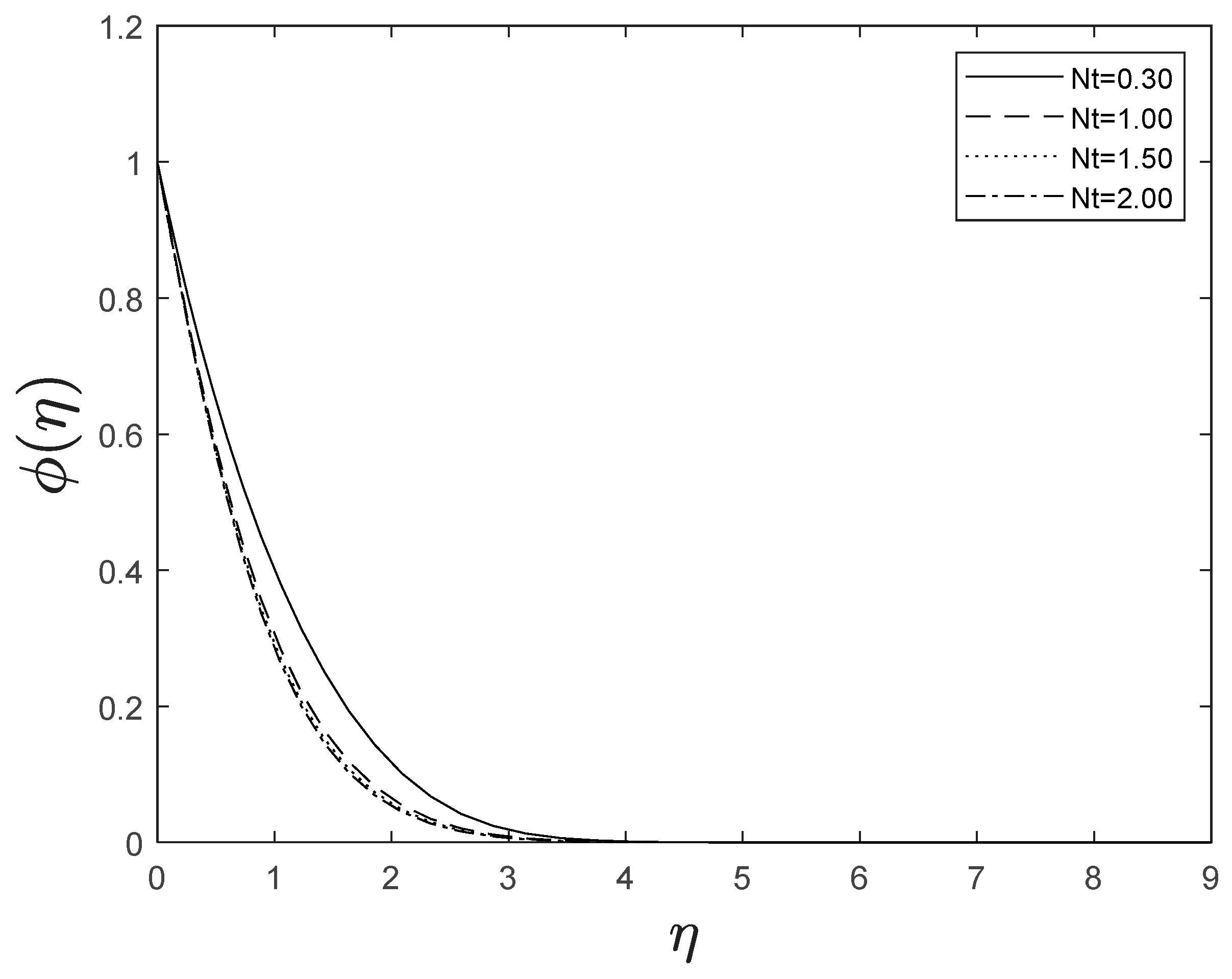
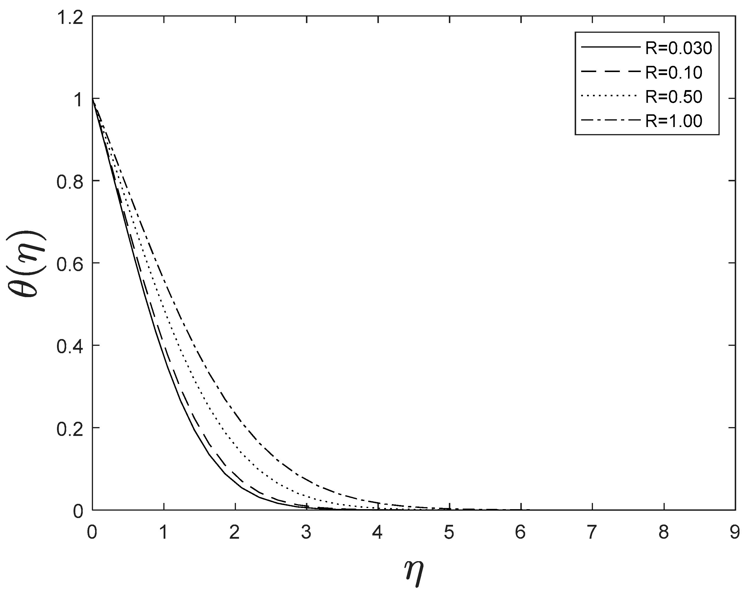
• Thermal radiation and thermophoresis parameters lead enhanced temperature.
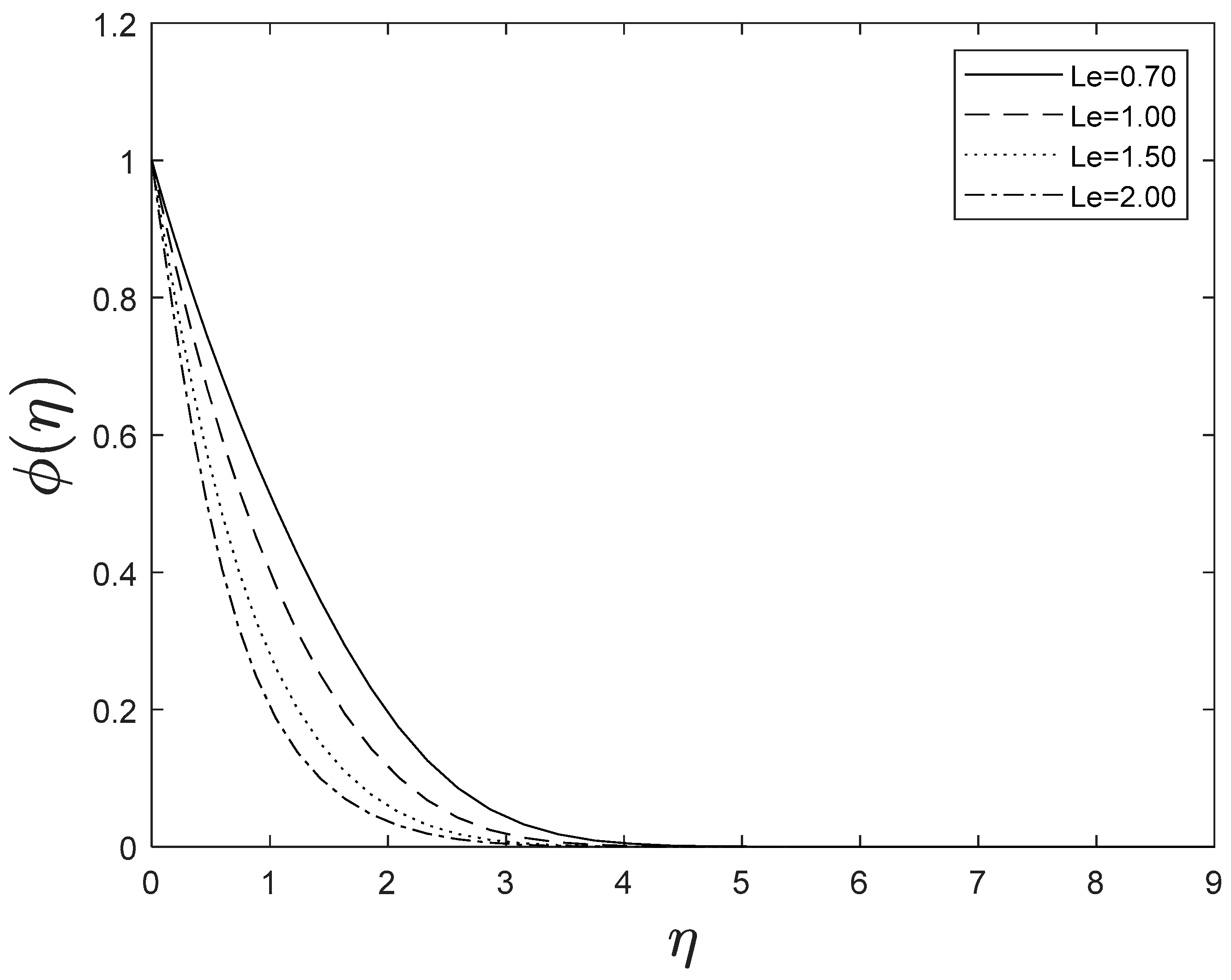
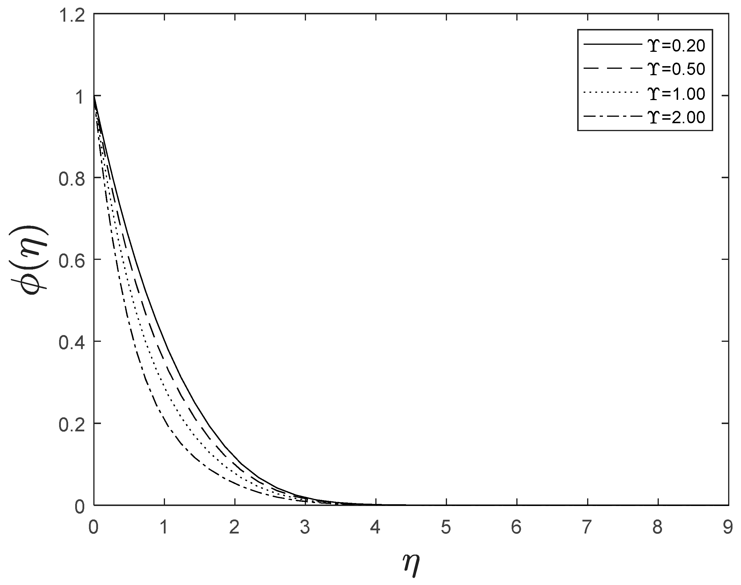
• The concentration profile lowers as both the Lewis number and the chemical reaction parameters expand.
• The rate of heat transfer elevates with $R$ and $\mathrm{Pr}$.
• The rate of mass transfer elevates with $Le$ and $\gamma$.

References

1. Abu-Nada, E.; Oztop, H.F. Effects of inclination angle on natural convection in enclosures filled with Cu-water nanofluid. Int. J. Heat Fluid Flow 2009, 30, 669–678. [Google Scholar] [CrossRef]
2. Zargartalebi, H.; Ghalambaz, M.; Noghrehabadi, A.; Chamkha, A.J. Stagnation point heat transfer of nanofluids toward stretching sheets with variable thermo-physical properties. Adv. Power Technol. 2015, 26, 819–829. [Google Scholar] [CrossRef]
3. Makinde, O.D.; Aziz, A. Boundary layer flow of a nanofluid past a stretching sheet with a convective boundary condition. Int. J. Therm. Sci. 2011, 50, 1326–1332. [Google Scholar] [CrossRef]
4. Mohamad, A.Q.; Khan, I.; Shafie, S. Unsteady free convection flow of rotating MHD second grade fluid in a porous medium over an oscillating plate. AIP Conf. Proceeding 2016, 1750, 030013. [Google Scholar]
5. Mbeledogu, I.U.; Ogulu, A. Heat and mass transfer of an unsteady MHD natural convection flow of a rotating fluid past a vertical flat plate in the presence of radiative heat transfer. Int. J. Heat Mass Transf. 2007, 50, 1902–1908. [Google Scholar] [CrossRef]
6. Salah, F.; Aziz, Z.A.; Ching, D.L.C. New exact solutions for MHD transient rotating flow of a second-grade fluid in a porous medium. J. Appl. Math. 2011, 823034, 2011. [Google Scholar] [CrossRef]
7. Sivanandam, S.; Marimuthu, B.; Alzahrani, A.K. Numerical study on influence of magnetic field and discrete heating on free convection in a porous container. Sci. Iran. 2022, 3063–3071. [Google Scholar]
8. Sivasankaran, S.; Narrein, K. Influence of geometry and magnetic field on convective flow of nanofluids in trapezoidal microchannel heat sink. Iran. J. Sci. Technol. Trans. Mech. Eng. 2020, 44, 373–382. [Google Scholar] [CrossRef]
9. Sivasankaran, S.; Malleswaran, A.; Bhuvaneswari, M.; Balan, P. Hydro-magnetic mixed convection in a lid-driven cavity with partially thermally active walls. Sci. Iran. 2017, 24, 153–163. [Google Scholar] [CrossRef]
10. Sivasankaran, S.; Ananthan, S.S.; Abdul Hakeem, A.K. Mixed convection in a lid-driven cavity with sinusoidal boundary temperature at the bottom wall in the presence of magnetic field. Sci. Iran. 2016, 23, 1027–1036. [Google Scholar] [CrossRef]
11. Sivasankaran, S.; Chandrapushpam, T.; Bhuvaneswari, M.; Karthikeyan, S.; Alzahrani, A.K. Effect of chemical reaction on double diffusive MHD squeezing copper water nanofluid flow between parallel plates. J. Mol. Liq. 2022, 368, 120768. [Google Scholar] [CrossRef]
12. Devi, L.; Niranjan, H.; Sivasankaran, S. Effects of chemical reactions, radiation, and activation energy on MHD buoyancy induced nano fluidflow past a vertical surface. Sci. Iran. 2022, 29, 90–100. [Google Scholar]
13. Yesodha, P.; Bhuvaneswari, M.; Sivasankaran, S.; Saravanan, K. Convective heat and mass transfer of chemically reacting fluids with activation energy along with Soret and Dufour effects. Mater. Today Proc. 2021, 42, 600–606. [Google Scholar] [CrossRef]
14. Sivanandam, S.; Marimuthu, B.; Arumugam, M.; Bhose, G. Stratification, slip and cross diffusion impacts on time depending convective stream with chemical reaction. Math. Model. Eng. Probl. 2019, 6, 581–588. [Google Scholar] [CrossRef]
15. Ariel, P.D. Hiemenz flow in hydromagnetics. Acta Mech. 1994, 103, 31–43. [Google Scholar] [CrossRef]
16. Motsa, S.S.; Khan, Y.; Shateyi, S. A new numerical solution of Maxwell fluid over a shrinking sheet in the region of a stagnation point. Math. Probl. Eng. 2012, 290615, 2012. [Google Scholar] [CrossRef]
17. Parand, K.; Lotfi, Y.; Rad, J.A. An efficient analytic approach for solving Hiemenz flow through a porous medium of a non-Newtonian Rivlin-Ericksen fluid with heat transfer. Nonlinear Eng. 2018, 7, 287–301. [Google Scholar] [CrossRef]
18. Waqas, H.; Imran, M.; Muhammad, T.; Sait, S.M.; Ellahi, R. On bio-convection thermal radiation in Darcy–Forchheimer flow of nanofluid with gyrotactic motile microorganism under Wu’s slip over stretching cylinder/plate. Int. J. Numer. Methods Heat Fluid Flow 2020, 31, 1520–1546. [Google Scholar] [CrossRef]
19. Farooq, U.; Waqas, H.; Imran, M.; Alghamdi, M.; Muhammad, T. On melting heat transport and nanofluid in a nozzle of liquid rocket engine with entropy generation. J. Mater. Res. Technol. 2021, 14, 3059–3069. [Google Scholar] [CrossRef]
20. Shahzad, A.; Imran, M.; Tahir, M.; Khan, S.A.; Akgül, A.; Abdullaev, S.; Yahia, I.S. Brownian motion and thermophoretic diffusion impact on Darcy-Forchheimer flow of bioconvective micropolar nanofluid between double disks with Cattaneo–Christov heat flux. Alex. Eng. J. 2023, 62, 1–15. [Google Scholar] [CrossRef]
21. Hamid, A.; Khan, M. Unsteady mixed convective flow of Williamson nanofluid with heat transfer in the presence of variable thermal conductivity and magnetic field. J. Mol. Liq. 2018, 260, 436–446. [Google Scholar]
22. Zhang, C.; Zheng, L.; Zhang, X.; Chen, G. MHD flow and radiation heat transfer of nanofluids in porous media with variable surface heat flux and chemical reaction. Appl. Math. Model. 2015, 39, 165–181. [Google Scholar] [CrossRef]
23. Pandey, A.K.; Kumar, M. Natural convection and thermal radiation influence on nanofluid flow over a stretching cylinder in a porous medium with viscous dissipation. Alex. Eng. J. 2017, 56, 55–62. [Google Scholar] [CrossRef]
24. Bhuvaneswari, M.; Sivasankaran, S.; Malarselvi, A.; Ganga, B. Radiation and cross diffusion on unsteady chemically reactive convective flow through an extended surface in heat generating porous medium. Int. J. Energy Technol. Policy 2021, 17, 494–509. [Google Scholar] [CrossRef]
25. Reddy, V.S.; Kandasamy, J.; Sivanandam, S. Impacts of Casson Model on Hybrid Nanofluid Flow over a Moving Thin Needle with Dufour and Soret and Thermal Radiation Effects. Math. Comput. Appl. 2022, 28, 2. [Google Scholar] [CrossRef]
26. Narayanaswamy, M.K.; Kandasamy, J.; Sivanandam, S. Go-MoS2/Water Flow over a Shrinking Cylinder with Stefan Blowing, Joule Heating, and Thermal Radiation. Math. Comput. Appl. 2022, 27, 110. [Google Scholar] [CrossRef]
27. Jagan, K.; Sivasankaran, S. Three-Dimensional Non-Linearly Thermally Radiated Flow of Jeffrey Nanoliquid towards a Stretchy Surface with Convective Boundary and Cattaneo–Christov Flux. Math. Comput. Appl. 2022, 27, 98. [Google Scholar] [CrossRef]
28. Uddin, M.J.; Khan, W.A.; Ismail, A.I. MHD forced convective laminar boundary layer flow of convectively heated moving vertical plate with radiation and transpiration effect. Plos ONE 2013, 8, 62664. [Google Scholar] [CrossRef]
29. Ahmed, M.A.M.; Mohammed, M.E.; Khidir, A.A. On linearization method to MHD boundary layer convective heat transfer with low pressure gradient. Propuls. Power Res. 2015, 4, 105–113. [Google Scholar] [CrossRef]
30. Salah, F.; Alzahrani, A.K.; Sidahmed, A.O.; Viswanathan, K.K. A note on thin-film flow of Eyring-Powell fluid on the vertically moving belt using successive linearization method. Int. J. Adv. Appl. Sci. 2019, 6, 17–22. [Google Scholar]
31. Yih, K.A. MHD forced convection flow adjacent to a non-isothermal wedge. Int. Comm. Heat Mass Transf. 1999, 26, 819–827. [Google Scholar] [CrossRef]
Figure 1. Physical model of the flow.
Mca 28 00021 g001
Figure 2. Effect of different values of M on f ( η ) .
Mca 28 00021 g002
Figure 3. Effect of different values of M on θ ( η ) .
Mca 28 00021 g003
Figure 4. Effect of different values of M on ϕ ( η ) .
Mca 28 00021 g004
Figure 5. Effect of different values of m on f ( η ) .
Mca 28 00021 g005
Figure 6. Effect of different values of m on θ ( η ) .
Mca 28 00021 g006
Figure 7. Effect of different values of m on ϕ ( η ) .
Mca 28 00021 g007
Figure 8. Effect of different values of V on f ( η ) .
Mca 28 00021 g008
Figure 9. Effect of different values of V on θ ( η ) .
Mca 28 00021 g009
Figure 10. Effect of different values of V on ϕ ( η ) .
Mca 28 00021 g010
Figure 11. Effect of different values of N b on θ ( η ) .
Mca 28 00021 g011
Figure 12. Effect of different values of N b on ϕ ( η ) .
Mca 28 00021 g012
Figure 13. Effect of different values of N t on θ ( η ) .
Mca 28 00021 g013
Figure 14. Effect of different values of N t on ϕ ( η ) .
Mca 28 00021 g014
Figure 15. Effect of different values of R on θ ( ζ ) .
Mca 28 00021 g015
Figure 16. Effect of different values of Pr on θ ( η ) .
Mca 28 00021 g016
Figure 17. Effect of different values of Q on θ ( η ) .
Mca 28 00021 g017
Figure 18. Effect of different values of L e on ϕ ( η ) .
Mca 28 00021 g018
Figure 19. Effect of different values of γ on ϕ ( η ) .
Mca 28 00021 g019
Figure 20. Effect of different values of Ω on f ( η ) .
Mca 28 00021 g020
Figure 21. Effect of different values of Ω on θ ( η ) .
Mca 28 00021 g021
Figure 22. Effect of different values of Ω on ϕ ( η ) .
Mca 28 00021 g022