
Forecasting Financial and Macroeconomic Variables Using an Adaptive Parameter VAR-KF Model

1
Advanced Research Center for Computational Simulation (ARCCoS), Department of Mathematics, Faculty of Science, Chiang Mai University, Chiang Mai 50200, Thailand
2
Centre of Excellence in Mathematics, CHE, Si Ayutthaya Road, Bangkok 10400, Thailand
*
Author to whom correspondence should be addressed.
Math. Comput. Appl. 2023, 28(1), 19; https://doi.org/10.3390/mca28010019
Submission received: 29 September 2022
/
Revised: 29 January 2023
/
Accepted: 1 February 2023
/
Published: 2 February 2023
(This article belongs to the Special Issue Statistical Inference in Linear Models)
Abstract
:The primary objective of this article is to present an adaptive parameter VAR-KF technique (APVAR-KF) to forecast stock market performance and macroeconomic factors. The method exploits a vector autoregressive model as a system identification technique, and the Kalman filter is served as a recursive state parameter estimation tool. A further development was designed by incorporating the GARCH model to quantify an automatic observation covariance matrix in the Kalman filter step. To verify the efficiency of our proposed method, we conducted an experimental simulation applied to the main stock exchange index, real effective exchange rate and consumer price index of Thailand and Indonesia from January 1997 to May 2021. The APVAR-KF method is generally shown to have a superior performance relative to the conventional VAR(1) model and the VAR-KF model with constant parameters.
1. Introduction
1.1. Motivation and Related Work
Due to an unprecedented increase in the uncertainty of economic and financial market activities, independent investors and policy makers require effective forecasting tools in order to facilitate more accurate decision plans. Numerous forecasting methods, ranging from univariate to multivariate time series models, have been developed to forecast stock market pricing and macroeconomic variables. Some of the most notable univariate techniques include autoregressive integrated moving average (ARIMA) models [1,2], artificial neural networks (ANNs) [3,4] and support vector machines (SVMs) [5,6]. In practice, economics and finance are correlated disciplines in which a change in one activity can cause uncertainty in the other. Macroeconomic fundamentals reflect the general economic environment and can influence the degree of variation in future cash flow in a stock market. Conversely, stock prices are often used as leading indicators that aggregate information about the economy’s direction. The existence of an association between macroeconomic indicators and stock prices has been extensively verified by several research studies [7,8,9]. Therefore, instead of using univariate time series forecasting techniques, multivariate time-series models are more suitable approaches for the predictability of macroeconomic variables, as well as stock indices.
Vector autoregressive (VAR) [10] models are multivariate time series techniques in which the dynamics of state variables can be expressed as a linear combination of past realizations. They are predominantly utilized for structural analysis and macroeconomic forecasting purposes because of their implementation’s simplicity and flexibility. Some studies that used VAR models for time series prediction include Suhasono et al. [11], who compared the forecasting performance between vector error correction modeling (VECM) and VAR models for ASEAN stock price indices. Öğünç [12] forecasted the inflation, nominal exchange rate and interest rate in Turkey through VAR variants. However, despite all of their advantages, the linearity assumption underlying VAR models can potentially lead to biased estimates, especially for a highly volatile time series. Several improvements for VAR models have been put forward to handle the inherent nonlinearity structure in data. One extensively used technique is to introduce drifting autoregressive coefficients to capture the presence of nonlinear effects in lagged dependent models. A time-varying parameter vector autoregression (TVP-VAR) model with stochastic volatility is a VAR-based approach in which the parameter estimation is calculated via the Markov chain Monte Carlo (MCMC) sampling algorithm [13]. D’Agostino et al. [14] compared the forecasting accuracy of nine time series methods in US inflation, unemployment and interest rates over the period of 1970–2007. They concluded that the TVP-VAR is the only method that can forecast all three variables accurately. Bekiros et al. [15] reported that using the TVP-VAR technique leads to a better forecasting ability than benchmark autoregression and random walk models when predicting the oil price movement with economic policy uncertainty being included. Kumar [16] examined the forecast ability of the ARIMA, VAR and TVP-VAR methods to predict the daily exchange rates of the Indian rupee against the U.S. dollar. The empirical results show that the TVP-VAR model outperforms other competing approaches. However, in the process of computing the posterior distribution of parameters of the traditional TVP-VAR model, the MCMC sampling algorithm requires a heavy computational burden in high-dimensional cases. To attenuate the curse of dimensionality, Korobilis [17] adopted a stochastic search algorithm using the Gibbs sampler to select potential variables that have a larger contribution to the forecasting accuracy. Many researchers make use of Bayesian data assimilation techniques, preferably the Kalman filtering (KF) [18], for the parameter estimation problem. Bekiros [19] exploited the KF algorithm and an extension of the univariate methodology framework for the parameter estimation in the TVP-VAR model to predict the monthly macroeconomic factors of the EU economy. Koop and Korobilis [20] introduced forgetting factors in the TVP-VAR model with parameters being recursively updated through the KF approach. Their purposed method leads to the scalability of the state-space estimator, and ultimately aids in a dimensionality reduction.
As far as the relationship between stock prices and macroeconomic fundamentals is concerned, it is accordingly plausible to include financial factors in macroeconomic forecasting and vice versa. Nevertheless, researchers tend to not forecast these variables simultaneously via multivariate time series models due to their different observed frequencies. In this work, we will present the hybrid VAR and KF method for the economic and financial trend prediction based on the monthly data. Motivated by Bekiros [19] and Koop and Korobilis [20], the model coefficients were sequentially updated through the joint state-parameter KF procedure rather than employing the filtering technique, particularly for the parameter estimation. The use of the KF model also involves the predetermination of noise covariances, where they are mostly constructed in an ad hoc manner that cannot accurately quantify model uncertainties under complex circumstances. Meanwhile, economic and financial time series are typically characterized by volatility clustering properties, or heteroscedasticity. We therefore enhanced our model with heteroscedastic noise by using a statistical technique to model an observation error covariance matrix and an average of sample covariances for a process error covariance matrix.
1.2. Contribution
The objectives of this paper are:
- We present a forecasting technique, the adaptive parameter VAR-KF (APVAR-KF) method, in which the state-space equations are constructed through the VAR model and the optimal state and parameter estimates are achieved using the KF approach.
- A generalized autoregressive conditional heteroskedasticity (GARCH) model was used to generate a measurement noise covariance matrix in the KF step in case of the presence of heteroscedasticity.
- The estimation and prediction performance of the APVAR-KF method was conducted and compared with VAR-based models with time-invariant parameters for the main stock exchange index and macroeconomic indicators in two selected emerging market economies: Thailand and Indonesia.
1.3. Article Structure
The remainder of this paper is organized as follows. Section 2 presents a detailed description of the proposed model, the APVAR-KF method, where a measurement noise covariance matrix was constructed through the multivariate GARCH with BEKK specification. Section 3 provides a comparative investigation of the estimation and prediction performances of the APVAR-KF and benchmark models for stock exchange index, real effective exchange rate and consumer price index of Thailand and Indonesia. Conclusions and discussion are drawn in Section 4.
2. Methodology
The Adaptive Parameter VAR-KF Model (APVAR-KF)
Consider the vector autoregressive (VAR) model for a stationary n-dimensional state vector at time instant k, . The VAR model of order p, denoted by VAR(p), has the form [10]
where is an intercept vector, for is an n × n matrix of autoregressive coefficients and η is an n-dimensional error vector.
Specifically, we assume the VAR model of order one, VAR(1), which can be expressed as
Equation (2) is treated as a state-space dynamical system in the KF method. This equation also signifies the validity of the linearity assumption of the KF through the VAR process. Let be the q-dimensional observation vector, which is related to the model state by the following equation:
where is an observation operator and is an observational error vector. To introduce time-variation parameters into the state Equation (2), we assume that the parameter transition equations follow a random walk process; therefore, for ,
where and for are coefficient components of matrices c and B, respectively, and and represent random noises, which are assumed to have the same distribution as .
By treating the parameters as additional state variables, they are concatenated to the model state vector in order to form a single vector , where and . The modified state propagation equation becomes
where is the zero-mean white noise with covariance matrix Q. The model coefficient matrix is formulated as
where denotes the j × j identity matrix and 0 is a zero matrix of appropriate size. The elements of are the parameter estimates from the previous time step, where the elements of are computed by the least square method.
The observation equation is subsequently modified as
where the observation operator and the observation noise term is assumed to be an independent and identically distributed observational Gaussian noise with associated error covariance matrix R. Since a volatility persistence is usually detected in financial and macroeconomic time series, we therefore incorporated a volatility feature through the observational covariance matrix R, which was modeled by the generalized autoregressive conditional heteroscedasticity (GARCH) process [21]. In particular, the multivariate BEKK [22] representation was selected to parametrize the GARCH model as the matrix R is guaranteed to be positive definite with unrestricted parameterizations. The BEKK(1,1) specification is written as
where D is restricted to be a lower triangular matrix representing constant components and A denotes an ARCH coefficient matrix that describes the effects of both own and cross fluctuations. The coefficient matrix M characterizes the GARCH effects reflecting the degree of its own and cross volatility persistence. To estimate the elements of these parameter matrices, we made use of the quasi-maximum likelihood [23] estimation, in which the likelihood function is given by
where T is the number of observations and θ denotes an unknown parameter vector.
Similar to the KF process, the APVAR-KF method comprises two steps: the forecast (prediction) and analysis (update) steps. In the forecast step, the aggregated state vector is propagated through the governing Equation (5). The resulting estimates are subsequently integrated with observation information in the analysis step to produce the optimal estimates. Superscripts f and a stand for forecast and analysis estimates, respectively, and we assumed the initial state estimate, , to be a Gaussian vector of zero mean with corresponding error covariance matrix . A description of how the error covariance matrices and Q in the KF step are attained is given in Section 3.
- The Forecast Step
Given that the analysis mean and its corresponding analysis covariance matrix are available, the forecast state can be obtained through
and the forecast covariance matrix
- The Analysis Step
The analysis state and analysis covariance are expressed as
where the Kalman gain matrix, G, determines the weight attributed to recent measurements, and is given by
3. Data and Simulation Results
To evaluate the efficiency of our proposed method, the monthly historical data used in this study include the stock market index, real effective exchange rate (REER) and consumer price index (CPI) of Thailand and Indonesia spanning from January 1997 to May 2021. The stock exchange of Thailand (SET) index data were collected from the Stock Exchange of Thailand website [24] and the REER and CPI data were acquired from the Bank of Thailand website [25], whereas the Jakarta stock exchange (JKSE) composite index was obtained from the investing.com database [26] and its REER and CPI data were taken from the Federal Reserve Economic Data (FRED) statistics [27]. The dataset is divided into two groups: the data from January 1997 to March 2021 were utilized for the training phase and data from April 2021 to May 2021 were treated as the testing phase. These raw data were transformed into monthly returns by taking the first logarithm difference. A z-score normalization [28] was subsequently applied to these return time series in order to adjust the range variation to comparable scales. The normalized returns were constructed by extracting the average from attribute values and dividing by the corresponding standard deviation.
3.1. Granger Causality Analysis
This section demonstrates an assessment of the interactions between different pairs of time series using the bivariate Granger causality test [29]. This analysis helps us to determine whether lagged values of one variable are linearly informative in forecasting another variable. Given two stationary variables and at time instant k, the bivariate Granger causality test follows a pair of regression equations:
where and are random disturbances and J is the maximum lag order. From the equations above, a unidirectional causality from the variable to variable is indicated if in Equation (14) is significantly different to zero by F-statistics whereas in the Equation (15) is not significant.
Table 1 presents the results of the Granger causality test for the direction of causality (F-statistics and p-value in parenthesis) among the normalized returns of the SET index, REER and CPI. The results show that the CPI does Granger-cause the SET index and REER at a 1% level of significance. Although the null hypothesis, which states that REER does not Granger-cause the CPI and SET index, is accepted, the null hypothesis in the opposite direction is rejected with a significance level of 1%. In the case of Indonesia, Table 2 reveals a two-way directional relationship between the CPI and JKSE index, and also between CPI and REER at a 5% level of significance. In addition, there is a unidirection causality running from the JKSE index to REER. With regard to the causality direction, the sufficient condition for the cointegration between two variables is that the Granger causality must exist in at least one direction [30]. Since our results indicate unidirectional causality between each pair of variables, it therefore suggests that all factors can be included in the model.
Table 3 presents some descriptive statistics of the monthly normalized return series. All normalized return series for both Thailand and Indonesia are highly leptokurtic and skewed with respect to the normal distribution, as indicated by the kurtosis and skewness measures. These results can be further confirmed by the Jarque–Bera test in which the normality hypothesis is rejected at a 1% significant level for all three variables. Similarly, the ARCH test rejects the null hypothesis of homoscedasticity at a 1% level of significance for all variables except the JKSE index with a 5% level of significance. This suggests the validation of the GARCH model in capturing the volatility interaction among variables, resulting in a plausible assumption of the observational covariance matrix in Equation (7). Since the VAR approach requires the data input to be stationary prior to the model implementation to avoid spurious regressions, the presence of unit roots was examined by a standard augmented Dickey–Fuller (ADF) test [31,32]. The ADF test well rejects the null hypothesis, with a statistical significance of 1% for every variable, which provides strong evidence of stationarity in the normalized return series for both countries.
3.2. Results
A prior requirement for a Kalman-filter-based recursive algorithm is the specification of an initial state vector, as well as its error covariance matrix. At the initial time instant k = 1, we used the actual initial data during our sample period along with the coefficients estimated from the ordinary least square method to be the elements of the initial state vector, . The corresponding error covariance matrix is assumed to be equal to the process noise covariance matrix Q, which is often assigned to be arbitrarily constant. We estimated the matrix Q through an average of sample covariances of the state prediction errors. The reference state vector at time instant k, , corresponds to a collection of the actual data and parameters evaluated from the VAR(1) model, and this gives . The noisy state-parameter vector was sampled from a Gaussian distribution with mean equal to , and the standard deviation was set to 25% of the reference values. The matrix Q was thus constructed using the following estimation:
where m is the number of time instants. There are three sample periods used to approximate the matrix Q, ranging from the first 12 months up to 60 months: January 1997–December 1997, January 1997–December 1999 and January 1997–December 2001. The resulting matrix Q applied to the APVAR-KF method was calculated on a statistical basis through the use of Monte Carlo simulations; that is, the matrix Q was determined by taking an average of over 50 experiments for each time instant. The results presented for the APVAR-KF method were obtained from the best-tuned values of the matrices and Q, which relied on the optimal achievable values of MAPE in the training period.
To demonstrate the performance of the APVAR-KF method in estimation and prediction, the classical vector autoregressive model of order one, VAR(1), was taken as a benchmark scheme. Meanwhile, an augmentation between the VAR model and KF with fixed model coefficients in Equation (2), the VAR-KF method, was additionally computed to illustrate the effects of a two-step procedure with and without time-variant model parameters upon the forecasting accuracy. The mean absolute percentage error (MAPE) and root mean square error (RMSE) were used as the performance evaluation indicators. They are formulated as follows:
and
where T is the total number of simulations, represents the actual measured data and denotes the estimated value.
Table 4 displays the estimation efficiency during the training period through the MAPE and RMSE statistics. According to MAPE and RMSE measures, both hybrid models have a superior estimation performance to the single model with lower MAPE and RMSE values for all variables of both countries. In the case of Thailand, the average MAPE values of VAR(1), VAR-KF and APVAR-KF models are 2.3460%, 2.0556% and 1.4089%, respectively. The VAR-KF approach reduces MAPE and RMSE values by over 10% compared to the benchmark model, whereas those of APVAR-KF by up to 40%. The same estimation pattern can be seen for Indonesia, where the overall improvement when using hybrid models is above 40%. These findings suggest that, by augmenting the Kalman filter in the VAR model, a significant improvement in the estimation accuracy is attained. When comparing among hybrid models, the APVAR-KF model exhibits better MAPE and RMSE values for all variables. The APVAR-KF model improves the quality of the overall estimation by approximately 30% for Thailand and approximately 6% for Indonesia regarding the MAPE values.
To assess the predictability using initial states acquired from three models, the state estimates in March 2021 were treated as the initial state vector for the underlying dynamical Equation (2) to forecast the state values of April 2021 and May 2021 (the testing phase). There are two different scenarios with respect to the model coefficients. The coefficients remain unchanged from the training phase for the VAR(1) and VAR-KF approaches, whereas those that relied on the APVAR-KF method are based on the parameter estimates in March 2021.
Table 5 demonstrates the forecasting performance in April 2021 of three models in terms of MAPE and RMSE criteria. The hybrid models in comparison with the VAR(1) model for Thailand yield a higher forecasting accuracy for all factors, with the average MAPE being 0.8303% and 0.6213%. These are, respectively, equivalent to a 18.8695% and 39.2900% improvement for the VAR-KF and APVAR-KF models, with the SET index being best improved. Similarly, both VAR-KF and APVAR-KF models achieve a better performance than the benchmark method for Indonesia, with a considerable improvement in the REER variable. Most errors attained from the APVAR-KF model are less than those of the VAR-KF method, except the REER variable of Indonesia, where the errors of using time-variant parameters are slightly greater than using fixed parameters. This indicates that the first time step prediction can predominantly be improved by exploiting the adjustable model parameters.
Table 6 reports the prediction efficiency of May 2021 forecasts. The VAR-KF and APVAR-KF models continue to outperform the traditional VAR(1) method for Thailand, with lower errors for all variables. By comparing among different hybrid algorithms, the APVAR-KF model provides better results for the REER and CPI, with a lower average MAPE of 0.8725%. Nevertheless, a different result arises for Indonesia, where the REER forecasts of the two-step methods are worse than the VAR(1) model despite the fact that the JKSE index and CPI errors achieved by the APVAR-KF technique are lowest among all of the individual algorithms. The predicted values for June 2021 are not shown in this report, considering that the error trends are similar to those in May 2021. The APVAR-KF model remains providing superior predictions for all variables of Thailand and for the main stock market price index of Indonesia.
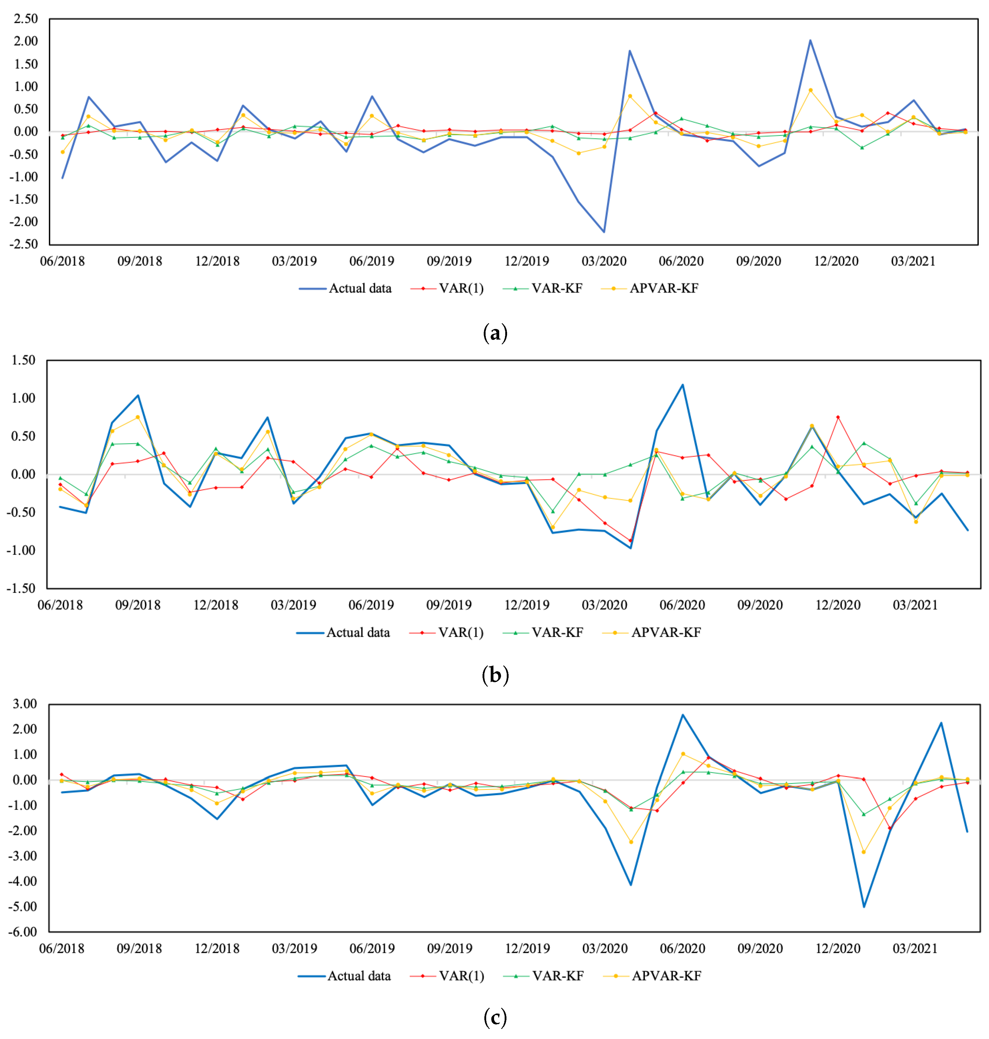
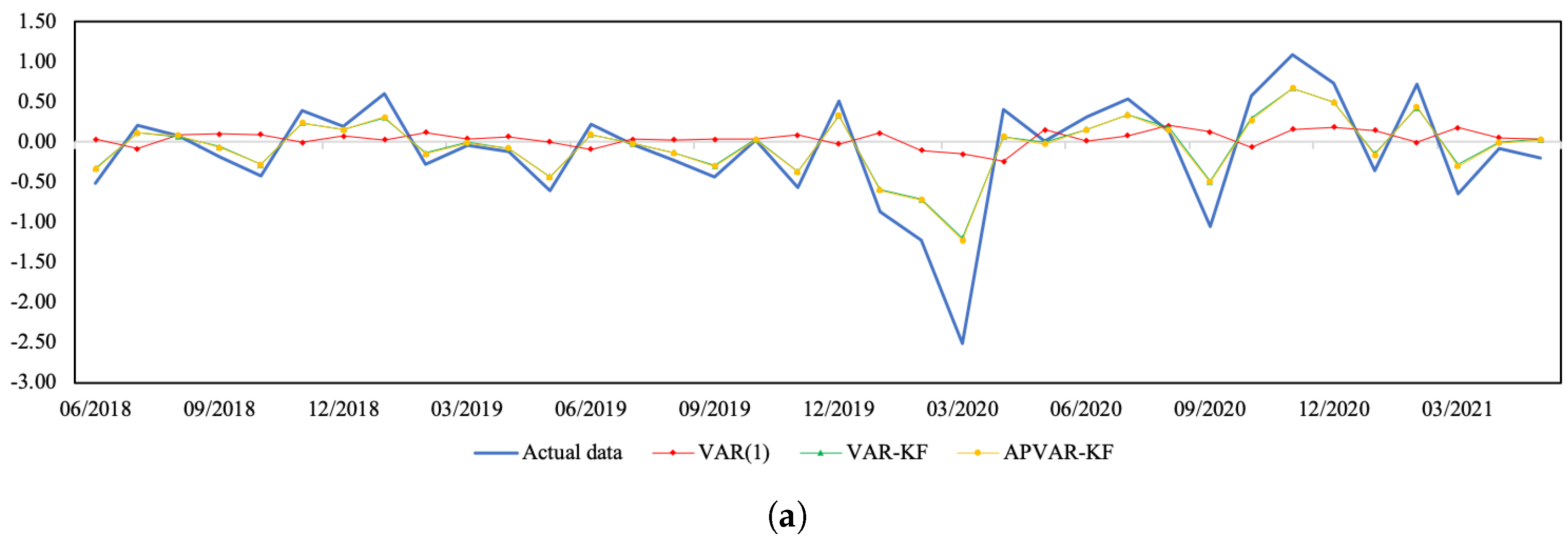
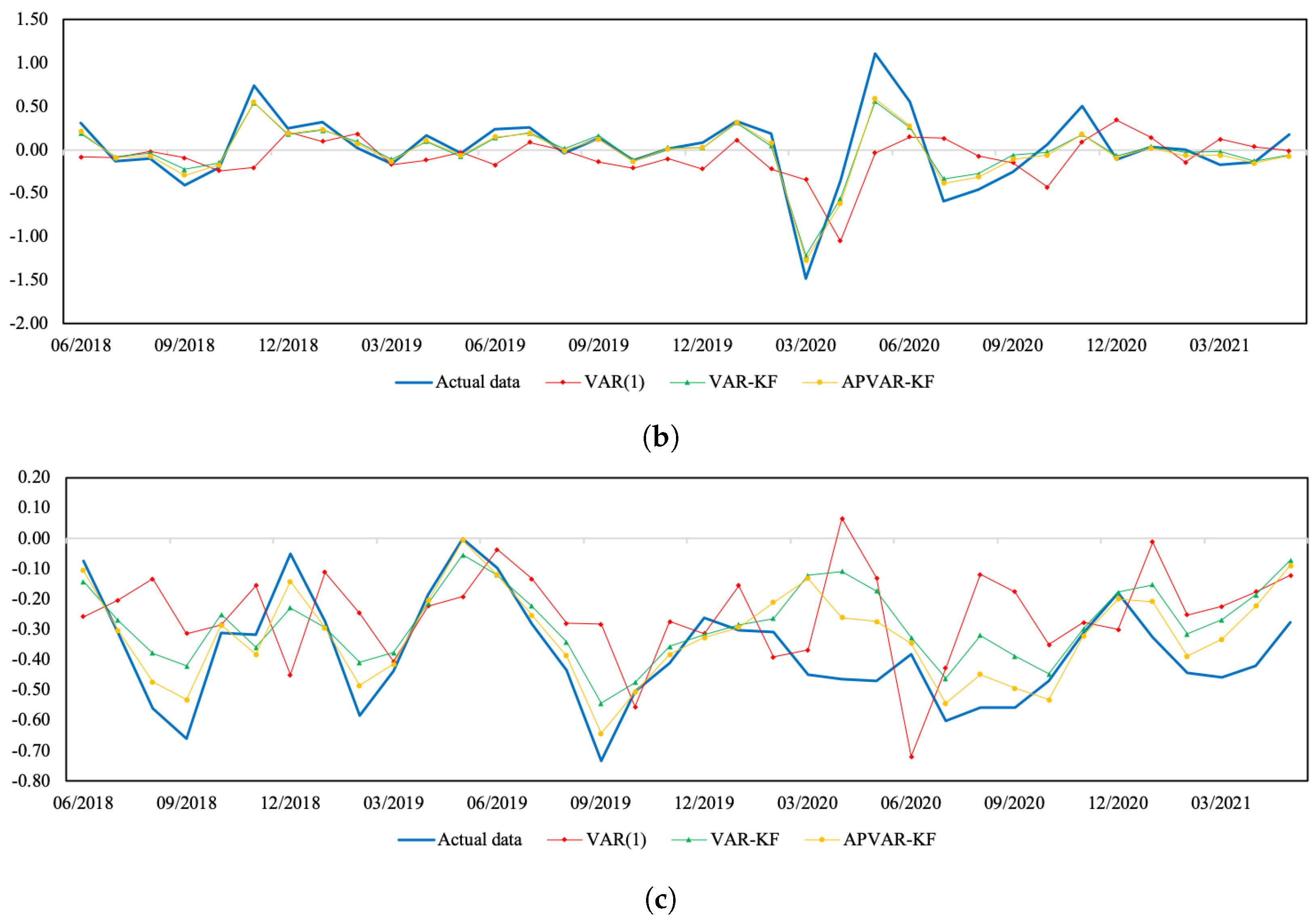
Figure 1 and Figure 2 depict a visual comparison between the normalized return estimates and actual data of all three variables of Thailand and Indonesia from July 2018 to May 2021. The plots of actual data and their corresponding estimates over the whole study period can be seen in Figure A1 and Figure A2. The discrepancy between the estimated values derived from all approaches and actual data appears to be minor over the tranquil period. In the course of the COVID-19 outbreak, when drastic changes in economic and financial situations took place, the APVAR-KF method performs best in capturing these abrupt changes in all variables, followed by the VAR-KF and VAR(1) models. These results may reflect that a variation in parameters allows the model to better track the actual data, especially during times of high uncertainty. This may be due to that fact that the coefficients of a model system are sequentially updated using recent observations, causing the underlying model to be able to forecast abruptly changing trends. For Indonesia, it appears that the forecasting results derived from the hybrid models exhibit similar increasing trends to the REER actual data, with relatively lower slopes during the testing phase, whereas the opposite trend direction pattern is found in the VAR(1) method. Although the results in Table 6 indicate a better REER forecasting ability when using the VAR(1) model, a further examination of how the trend direction changes can be of importance.
4. Conclusions and Discussion
Forecasting economic and financial time series can have substantial implications for the implementation of monetary policies and regulations and for an individual investor’s investment decision. This paper is designed to model and forecast the complex interactions between the economic factors and financial market by introducing the hybrid APVAR-KF model for joint state parameter estimation. The method combines the Kalman filter with the VAR model, in which, the observational error covariance matrix is implemented using the multivariate BEKK-GARCH representation.
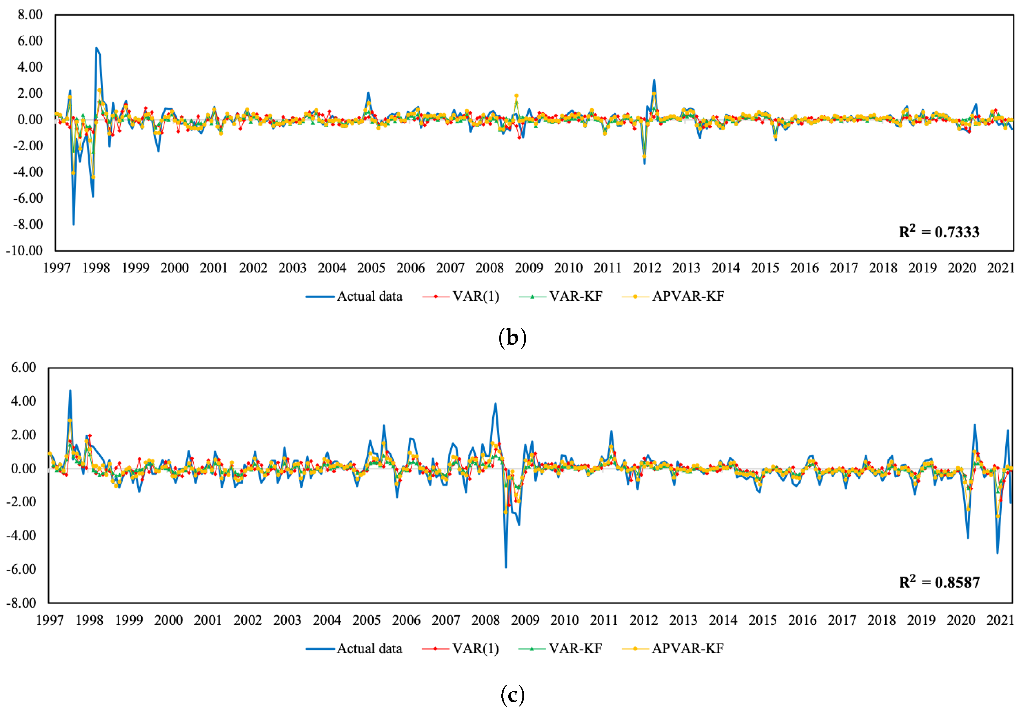
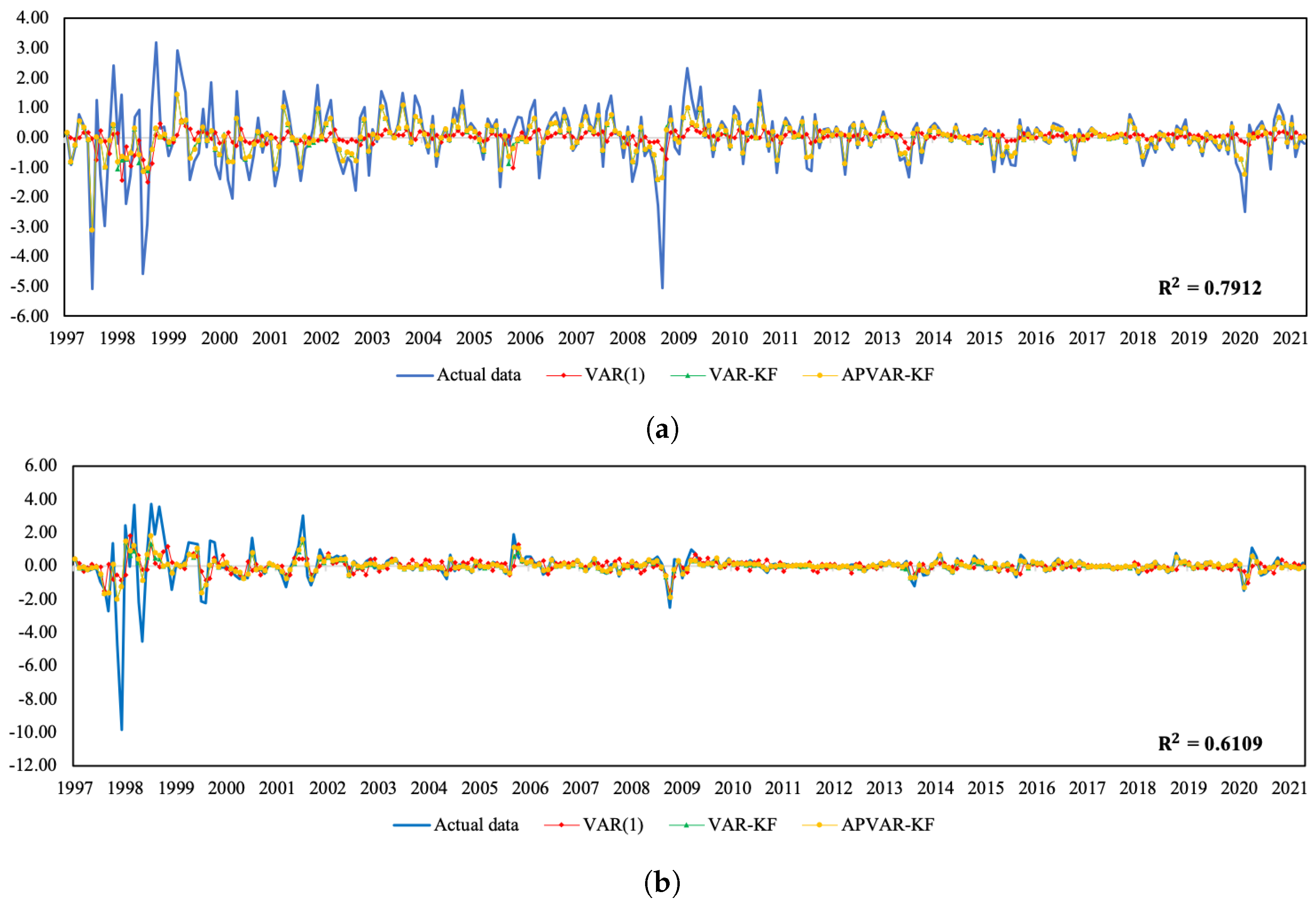
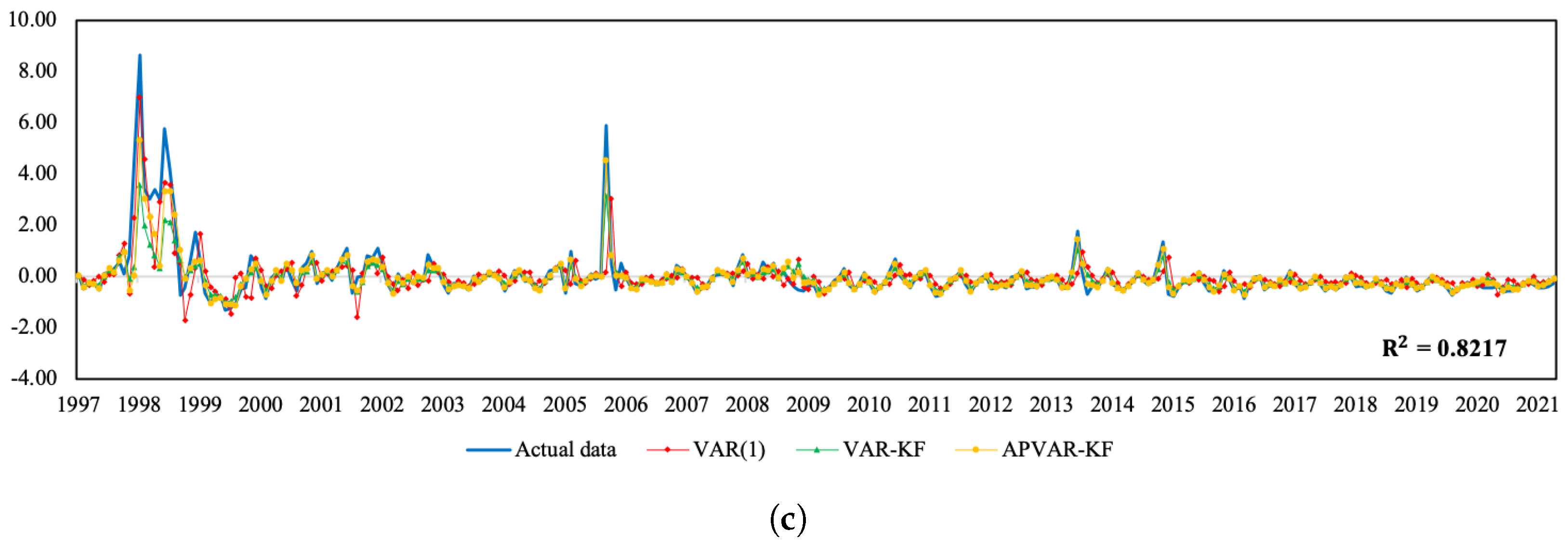
In addition to providing the best estimation performance, the APVAR-KF technique tends to offer satisfactory short-term predictions and future trend patterns. As presented in Figure A1 and Figure A2, the coefficient of determination (R-square) values between the observed data and the estimates of the APVAR-KF model range from 0.6109 to 0.8713, or 61.09% to 87.13%, which suggests that our proposed model has the ability to capture the dynamics of economic and financial time series.
In this regard, the benefits of the APVAR-KF model in estimation and prediction may be attributed to two reasons. The first reason is that this is a two-step process in which the Kalman filter provides a mechanism that can extract discriminative information from the training data. Another reason is that adaptive parameters can enhance the hybrid performance, creating a plausible model structure that adjusts to a change in state characteristics over time. This is considerably beneficial, especially when an unexpected fluctuation caused by economic instability occurs. Despite the favorable results of this study, the assumption of lag one in the VAR step can be a limitation of the method. The VAR model specification with higher lag orders and an inclusion of more macro factors, can be of particular interest. However, this is an apparent tradeoff problem between a more elaborate model and a heavy computational burden due to a large dimension of the state space. Ensemble-based filters that allow for the error covariance matrices to be computed without a moment closure assumption can potentially provide computational feasibility and efficiency. Due to the sensitivity of the process noise covariance Q to the prediction performance of the APVAR-KF approach, another challenge concerns the selection criteria of the matrix Q. In this work, we used the sample covariance calculated from a particular time period to represent the process noise statistics. Instead, other techniques, including the adaptive Q algorithm, covariance inflation and some rigorous optimization approaches, can be adopted, especially under some complex and dynamic circumstances.
Author Contributions
N.P. and N.C. designed the research, implemented the numerical experiments and analyzed the results. N.C. wrote the manuscript and N.P. and N.C. approved the final manuscript. All authors have read and agreed to the published version of the manuscript.
Funding
This research was funded by the Research Fund for DPST Graduate with First Placement [Grant no. 029/2559], the Institute for the Promotion of Teaching Science and Technology (IPST), Thailand.
Acknowledgments
The authors would like to thank Thanasak Mouktonglang and Sompop Moonchai for their helpful insight and suggestions. This research was supported by Chiang Mai University and the Centre of Excellence in Mathematics, CHE, Thailand. Nawinda Chutsagulprom was supported by the Research Fund for DPST Graduate with First Placement [Grant no. 029/2559], the Institute for the Promotion of Teaching Science and Technology (IPST), Thailand, under the mentoring of Thanasak Mouktonglang.
Conflicts of Interest
The authors declare no conflict of interest.
Abbreviations
The following abbreviations are used in this manuscript:
| VAR | Vector Autoregressive Model |
| KF | Kalman Filter |
| GARCH | Generalized Autoregressive Conditional Heteroscedasticity |
| SET | Stock Exchange of Thailand |
| JKSE | Jakarta Stock Exchange Composite Index |
| REER | Real Effective Exchange Rate |
| CPI | Consumer Price Index |
| MAPE | Mean Absolute Percentage Error |
| RMSE | Root Mean Square Error |
Appendix A
Figure A1.
Plots of the actual data and the estimated values from three methods for Thailand. (a) Normalized SET index return; (b) normalized real effective exchange rate return; (c) normalized CPI return.
Figure A1.
Plots of the actual data and the estimated values from three methods for Thailand. (a) Normalized SET index return; (b) normalized real effective exchange rate return; (c) normalized CPI return.


Figure A2.
Plots of the actual data and the estimated values from three methods for Indonesia. (a) Normalized SET index return; (b) normalized real effective exchange rate return; (c) normalized CPI return.
Figure A2.
Plots of the actual data and the estimated values from three methods for Indonesia. (a) Normalized SET index return; (b) normalized real effective exchange rate return; (c) normalized CPI return.


References
- Ariyo, A.A.; Adewumi, A.O.; Ayo, C.K. Stock price prediction using the ARIMA model. In Proceedings of the 2014 UKSim-AMSS 16th International Conference on Computer Modelling and Simulation, Cambridge, UK, 26–28 March 2014; pp. 106–112. [Google Scholar] [CrossRef]
- Junior, P.R.; Salomon, F.L.R.; de Oliveira Pamplona, E. ARIMA: An applied time series forecasting model for the Bovespa stock index. Appl. Math. 2014, 5, 3383. [Google Scholar] [CrossRef]
- Moghaddam, A.H.; Moghaddam, M.H.; Esfandyari, M. Stock market index prediction using artificial neural network. J. Econ. Financ. Adm. Sci. 2016, 21, 89–93. [Google Scholar] [CrossRef]
- Qiu, M.; Song, Y.; Akagi, F. Application of artificial neural network for the prediction of stock market returns: The case of the Japanese stock market. Chaos Solit. Fract. 2016, 85, 1–7. [Google Scholar] [CrossRef]
- Shen, S.; Jiang, H.; Zhang, T. Stock Market Forecasting Using Machine Learning Algorithms; Department of Electrical Engineering, Stanford University: Stanford, CA, USA, 2012; pp. 1–5. [Google Scholar]
- Ren, R.; Wu, D.D.; Liu, T. Forecasting stock market movement direction using sentiment analysis and support vector machine. IEEE Syst. J. 2018, 13, 760–770. [Google Scholar] [CrossRef]
- Yang, E.; Kim, S.H.; Kim, M.H.; Ryu, D. Macroeconomic shocks and stock market returns: The case of Korea. Appl. Econ. 2018, 50, 757–773. [Google Scholar] [CrossRef]
- Antonakakis, N.; André, C.; Gupta, R. Dynamic spillovers in the United States: Stock market, housing, uncertainty, and the macroeconomy. South. Econ. J. 2016, 83, 609–624. [Google Scholar] [CrossRef]
- Vrugt, E.B. US and Japanese macroeconomic news and stock market volatility in Asia-Pacific. Pac.-Basin Financ. J. 2009, 17, 611–627. [Google Scholar] [CrossRef]
- Sims, C.A. Macroeconomics and reality. Econom. J. Econom. Soc. 1980, 1–48. [Google Scholar] [CrossRef]
- Suharsono, A.; Aziza, A.; Pramesti, W. Comparison of vector autoregressive (VAR) and vector error correction models (VECM) for index of ASEAN stock price. AIP Publ. 2017, 1913, 020032. [Google Scholar] [CrossRef] [Green Version]
- Öğünç, F.; Akdoğan, K.; Başer, S.; Chadwick, M.G.; Ertuğ, D.; Hülagü, T.; Kösem, S.; Özmen, M.U.; Tekatlı, N. Short-term inflation forecasting models for Turkey and a forecast combination analysis. Econ. Model. 2013, 33, 312–325. [Google Scholar] [CrossRef]
- Primiceri, G.E. Time varying structural vector autoregressions and monetary policy. Rev. Econ. Stud. 2005, 72, 821–852. [Google Scholar] [CrossRef]
- D’Agostino, A.; Gambetti, L.; Giannone, D. Macroeconomic forecasting and structural change. J. Appl. Econom. 2013, 28, 82–101. [Google Scholar] [CrossRef]
- Bekiros, S.; Gupta, R.; Paccagnini, A. Oil price forecastability and economic uncertainty. Econ. Lett. 2015, 132, 125–128. [Google Scholar] [CrossRef]
- Kumar, M. A time-varying parameter vector autoregression model for forecasting emerging market exchange rates. Int. J. Econ. Sci. Appl. Res. 2010, 3, 21–39. [Google Scholar]
- Korobilis, D. VAR forecasting using Bayesian variable selection. J. Appl. Econom. 2013, 28, 204–230. [Google Scholar] [CrossRef]
- Kalman, R.E. A new approach to linear filtering and prediction problems. J. Basic Eng. 1960, 82, 35–45. [Google Scholar] [CrossRef]
- Bekiros, S. Forecasting with a state space time-varying parameter VAR model: Evidence from the Euro area. Econ. Model. 2014, 38, 619–626. [Google Scholar] [CrossRef]
- Koop, G.; Korobilis, D. Large time-varying parameter VARs. J. Econom. 2013, 177, 185–198. [Google Scholar] [CrossRef]
- Bollerslev, T. Generalized autoregressive conditional heteroskedasticity. J. Econom. 1986, 31, 307–327. [Google Scholar] [CrossRef]
- Engle, R.F.; Kroner, K.F. Multivariate simultaneous generalized ARCH. Econom. Theory 1995, 11, 122–150. [Google Scholar] [CrossRef]
- Bollerslev, T.; Wooldridge, J.M. Quasi-maximum likelihood estimation and inference in dynamic models with time-varying covariances. Econom. Rev. 1992, 11, 143–172. [Google Scholar] [CrossRef]
- Stock Exchange of Thailand Website. 2021. Available online: https://classic.set.or.th/en/market/market_statistics.html (accessed on 5 October 2021).
- Bank of Thailand Website. 2021. Available online: https://bot.or.th (accessed on 5 October 2021).
- Investing Website. 2022. Available online: https://www.investing.com/indices/idx-composite-historical-data (accessed on 5 October 2021).
- Federal Reserve Economic Data website. 2022. Available online: https://fred.stlouisfed.org/ (accessed on 5 October 2021).
- Kang, S.H.; Yoon, S.M. Long memory features in the high frequency data of the Korean stock market. Phys. Stat. Mech. Its Appl. 2008, 387, 5189–5196. [Google Scholar] [CrossRef]
- Granger, C.W. Investigating causal relations by econometric models and cross-spectral methods. Econom. J. Econom. Soc. 1969, 424–438. [Google Scholar] [CrossRef]
- Engle, R.F.; Granger, C.W. Co-integration and error correction: Representation, estimation, and testing. Econom. J. Econom. Soc. 1987, 55, 251–276. [Google Scholar] [CrossRef]
- Dickey, D.A.; Fuller, W.A. Distribution of the estimators for autoregressive time series with a unit root. J. Am. Stat. Assoc. 1979, 74, 427–431. [Google Scholar] [CrossRef]
- Dickey, D.A.; Fuller, W.A. Likelihood ratio statistics for autoregressive time series with a unit root. Econom. J. Econom. Soc. 1981, 49, 1057–1072. [Google Scholar] [CrossRef]
Figure 1.
A comparison between the actual data and the estimated values from three methods for Thailand during July 2018–May 2021. (a) Normalized SET index return; (b) normalized real effective exchange rate return; (c) normalized CPI return.
Figure 1.
A comparison between the actual data and the estimated values from three methods for Thailand during July 2018–May 2021. (a) Normalized SET index return; (b) normalized real effective exchange rate return; (c) normalized CPI return.

Figure 2.
A comparison between the actual data and the estimated values from three methods for Indonesia during July 2018–May 2021. (a) Normalized JKSE index return; (b) normalized real effective exchange rate return; (c) normalized CPI return.
Figure 2.
A comparison between the actual data and the estimated values from three methods for Indonesia during July 2018–May 2021. (a) Normalized JKSE index return; (b) normalized real effective exchange rate return; (c) normalized CPI return.


Table 1.
Pairwise Granger causality test of the normalized return series of Thailand.
| Dependent Variable | F-Statistics Test | ||
|---|---|---|---|
| SET Index (Prob. Values) | REER (Prob. Values) | CPI (Prob. Values) | |
| SET index | 21.2505 | 1.6713 | |
| (0.0000) *** | (0.1971) | ||
| REER | 1.0583 | 0.2262 | |
| (0.3045) | (0.6347) | ||
| CPI | 10.6046 | 15.7289 | |
| (0.0013) *** | (0.0000) *** | ||
Notes: *** denotes significance at the 1%.
Table 2.
Pairwise Granger causality test of the normalized return series of Indonesia.
| Dependent Variable | F-Statistics Test | ||
|---|---|---|---|
| JKSE Index (Prob. Values) | REER (Prob. Values) | CPI (Prob. Values) | |
| JKSE index | 21.0083 | 4.3218 | |
| (0.0000) *** | (0.0385) ** | ||
| REER | 0.5960 | 93.2368 | |
| (0.4408) | (0.0000) *** | ||
| CPI | 6.5980 | 5.8258 | |
| (0.0107) ** | (0.0164) ** | ||
Notes: ** and *** denote significance at the 5% and 1%, respectively.
Table 3.
Descriptive statistics of normalized return series.
| Variable | Stock Index | REER | CPI |
|---|---|---|---|
| Thailand | |||
| Skewness | −0.4037 | −1.7799 | −0.8021 |
| Kurtosis | 6.1646 | 25.6633 | 11.7886 |
| Maximum | 3.5321 | 5.5006 | 4.6552 |
| Minimum | −4.5314 | −7.9811 | −5.8710 |
| Jarque–Bera | 128.8900 *** | 6359.4434 *** | 964.3984 *** |
| ARCH test | 8.1017 *** | 37.2224 *** | 29.8895 *** |
| ADF | −11.2860 *** | −11.1884 *** | −9.4615 *** |
| Indonesia | |||
| Skewness | −1.2042 | −3.5107 | 4.7035 |
| Kurtosis | 8.6444 | 39.2024 | 31.6584 |
| Maximum | 3.1898 | 3.6852 | 8.6086 |
| Minimum | −5.0722 | −9.8602 | −1.3426 |
| Jarque–Bera | 455.0480 *** | 16432.3347 *** | 10993.3566 *** |
| ARCH test | 5.7372 ** | 20.9877 *** | 47.8145 *** |
| ADF | −12.2780 *** | −12.8950 *** | −7.2100 *** |
Notes: ** and *** denote significance at the 5% and 1%, respectively.
Table 4.
Mean absolute percentage errors and root mean square errors during the training phase (January 1997–March 2021).
Table 4.
Mean absolute percentage errors and root mean square errors during the training phase (January 1997–March 2021).
| Variable | MAPE | RMSE | ||||
|---|---|---|---|---|---|---|
| VAR(1) | VAR-KF | APVAR-KF | VAR(1) | VAR-KF | APVAR-KF | |
| Thailand | ||||||
| SET index | 5.5705 | 5.0223 | 3.4655 | 54.8660 | 50.5360 | 34.8130 |
| REER | 1.1547 | 0.8920 | 0.5892 | 2.0094 | 1.5422 | 1.1419 |
| CPI | 0.3129 | 0.2525 | 0.1721 | 0.4243 | 0.3529 | 0.2415 |
| Average error | 2.3460 | 2.0556 | 1.4089 | 31.6991 | 29.1913 | 20.1106 |
| Indonesia | ||||||
| JKSE index | 5.2524 | 2.8055 | 2.7349 | 158.7900 | 70.9540 | 69.4390 |
| REER | 2.7593 | 1.6239 | 1.4992 | 3.3597 | 2.3697 | 2.2680 |
| CPI | 0.5095 | 0.3356 | 0.2279 | 0.4702 | 0.2827 | 0.1906 |
| Average error | 2.8404 | 1.5883 | 1.4873 | 91.6984 | 40.9885 | 40.1122 |
Table 5.
Mean absolute percentage errors and root mean square errors of April 2021.
| Variable | MAPE | RMSE | ||||
|---|---|---|---|---|---|---|
| VAR(1) | VAR-KF | APVAR-KF | VAR(1) | VAR-KF | APVAR-KF | |
| Thailand | ||||||
| SET index | 1.0765 | 0.6936 | 0.1845 | 17.0420 | 10.9800 | 2.9212 |
| REER | 0.6606 | 0.6199 | 0.5341 | 0.7087 | 0.6650 | 0.5730 |
| CPI | 1.3333 | 1.1776 | 1.1454 | 1.3397 | 1.1832 | 1.1509 |
| Average error | 1.0235 | 0.8303 | 0.6213 | 9.8780 | 6.3876 | 1.8427 |
| Indonesia | ||||||
| JKSE index | 0.9919 | 0.5629 | 0.4873 | 59.4720 | 33.7510 | 29.2170 |
| REER | 0.9884 | 0.0666 | 0.0844 | 0.8703 | 0.0586 | 0.0743 |
| CPI | 0.3198 | 0.3065 | 0.2595 | 0.3773 | 0.3616 | 0.3062 |
| Average error | 0.7667 | 0.3120 | 0.2771 | 34.3405 | 19.4873 | 16.8694 |
Table 6.
Mean absolute percentage errors and root mean square errors of May 2021.
| Variable | MAPE | RMSE | ||||
|---|---|---|---|---|---|---|
| VAR(1) | VAR-KF | APVAR-KF | VAR(1) | VAR-KF | APVAR-KF | |
| Thailand | ||||||
| SET index | 0.8830 | 0.2855 | 0.3552 | 14.0720 | 4.5503 | 5.6597 |
| REER | 2.4384 | 2.3650 | 2.2208 | 2.5718 | 2.4943 | 2.3423 |
| CPI | 0.2959 | 0.0811 | 0.0415 | 0.2946 | 0.0807 | 0.0413 |
| Average error | 1.2058 | 0.9105 | 0.8725 | 8.2608 | 2.9963 | 3.5365 |
| Indonesia | ||||||
| JKSE index | 2.8246 | 2.3965 | 2.2698 | 167.9900 | 142.5300 | 135.0000 |
| REER | 0.0547 | 1.2434 | 1.4632 | 0.0486 | 1.1049 | 1.3002 |
| CPI | 0.5235 | 0.5752 | 0.5049 | 0.6197 | 0.6809 | 0.5977 |
| Average error | 1.1343 | 1.4050 | 1.4126 | 96.9897 | 82.2931 | 77.9467 |
Disclaimer/Publisher’s Note: The statements, opinions and data contained in all publications are solely those of the individual author(s) and contributor(s) and not of MDPI and/or the editor(s). MDPI and/or the editor(s) disclaim responsibility for any injury to people or property resulting from any ideas, methods, instructions or products referred to in the content. |
© 2023 by the authors. Licensee MDPI, Basel, Switzerland. This article is an open access article distributed under the terms and conditions of the Creative Commons Attribution (CC BY) license (https://creativecommons.org/licenses/by/4.0/).
Share and Cite
MDPI and ACS Style
Promma, N.; Chutsagulprom, N. Forecasting Financial and Macroeconomic Variables Using an Adaptive Parameter VAR-KF Model. Math. Comput. Appl. 2023, 28, 19. https://doi.org/10.3390/mca28010019
AMA Style
Promma N, Chutsagulprom N. Forecasting Financial and Macroeconomic Variables Using an Adaptive Parameter VAR-KF Model. Mathematical and Computational Applications. 2023; 28(1):19. https://doi.org/10.3390/mca28010019
Chicago/Turabian StylePromma, Nat, and Nawinda Chutsagulprom. 2023. "Forecasting Financial and Macroeconomic Variables Using an Adaptive Parameter VAR-KF Model" Mathematical and Computational Applications 28, no. 1: 19. https://doi.org/10.3390/mca28010019