Many-Objectives Optimization: A Machine Learning Approach for Reducing the Number of Objectives

Abstract

Solving real-world multi-objective optimization problems using Multi-Objective Optimization Algorithms becomes difficult when the number of objectives is high since the types of algorithms generally used to solve these problems are based on the concept of non-dominance, which ceases to work as the number of objectives grows. This problem is known as the curse of dimensionality. Simultaneously, the existence of many objectives, a characteristic of practical optimization problems, makes choosing a solution to the problem very difficult. Different approaches are being used in the literature to reduce the number of objectives required for optimization. This work aims to propose a machine learning methodology, designated by FS-OPA, to tackle this problem. The proposed methodology was assessed using DTLZ benchmarks problems suggested in the literature and compared with similar algorithms, showing a good performance. In the end, the methodology was applied to a difficult real problem in polymer processing, showing its effectiveness. The algorithm proposed has some advantages when compared with a similar algorithm in the literature based on machine learning (NL-MVU-PCA), namely, the possibility for establishing variable–variable and objective–variable relations (not only objective–objective), and the elimination of the need to define/chose a kernel neither to optimize algorithm parameters. The collaboration with the DM(s) allows for the obtainment of explainable solutions.

1. Introduction

Real-world optimization problems are usually multiobjective, in which multiple conflicting objectives must be taken into account simultaneously. Manly, there are two ways to tackle these types of problems, scalarization functions and population-based algorithms. The use of scalarization functions presented some drawbacks, which led to the development of population-based metaheuristics that use the concept of Pareto-dominance and niching to evolve a population of solutions in the direction of the Pareto-optimal front [1,2].

There are at least three basic types of population-based algorithms commonly employed to solve Multiobjective Optimization Problems MOPs, namely, evolutionary algorithms, swarm-based methods, and colony-based algorithms, which can use the dominance concept, the metric indicators, or the decomposition strategy [3]. In most of these algorithms, a random initial population of solutions is generated and the new populations are consecutively obtained by selection and variation strategies until a stop criterion is met. It is expected from this procedure that the successive populations evolve towards, or to a good approximation of, the Pareto-optimal frontier. In each one of these populations, complex relations exist between the Decision Variables (DVs) and the objectives, as well as between DVs and DVs and objectives and objectives.

These algorithms work well when the number of objectives is low; however, as the number of objectives grows, the percentage of non-dominated solutions decreases, making it difficult for an algorithm based on Pareto-dominance to work effectively, a problem that is known as the curse of dimensionality. There is no consensus on the number of objectives for which this problem occurs; some authors indicate this number as ten [4] and others as four [5], but in reality, these difficulties arise when the number of objectives is four or more.

Two different methods are used to deal with this problem, either using relaxed forms of Pareto optimality or reducing the number of objectives [5]. The reduction of the number of objectives is useful either for the search process or for the decision-making process during and/or at the end of the optimization.

In previous years, some work related to objective reduction for many objectives optimization was proposed in the literature, which can be sub-divided into four different categories: (i) methods in which the aim is to maintain the dominance relation for the non-dominated solutions [6,7]; (ii) methods based on unsupervised feature selection [8]; (iii) methods based into a comparative analysis between the results obtained when the number of objectives is reduced [9]; (iv) methods based on data mining [5,10,11,12]; and methods based on the use of multi-objective formulations [13]. These approaches will be presented in more detail here.

Brockoff and Zitzler [6,7] suggested the use of two different approaches for objectives reduction, which are based on the definition of two types of problems. The first problem aims to obtain the minimum objective subset that produces a certain error (δ), designated by δ-MOSS problem (δ- Minimum Objective Subset problem), and the second problem aims to obtain an objective subset of a predefined size (k) with the minimum possible error, designated by k-EMOSS problem. For each one of these cases, two algorithms were presented, an exact and a greedy algorithm, characterized for maintaining the dominance relation. They were tested using different knapsack problems and the DTLZ2, DTLZ5, and DTLZ7 benchmark problems for different numbers of objectives.

In López et al. [8], a methodology based on unsupervised feature selection was proposed to address the δ-MOSS and k-EMOSS problems. A correlation matrix obtained from the non-dominated set is used to divide the objective set into homogeneous neighbourhoods. Then, based on the idea that if the distance between the objectives is higher, this signifies that those objectives are more conflicting. Thus, only the objectives in the centre of those neighbourhoods are chosen and the others are discarded. The algorithms were validated by comparing the results obtained with those of the reference [7].

Singh et al. [9] proposed an algorithm, designated by the Pareto Corner Search Evolutionary Algorithm (PCSEA) that, instead of searching for the complete Pareto front, searches for the corners of the Pareto front based on a ranking scheme. Those solutions are used to identify the relevant objectives and the others are discarded. Some benchmark problems and two engineering problems were used to show the performance of the methodology proposed.

Deb and Saxena [10] suggested an approach based on Principal Component Analysis (PCA) for the same purpose of objectives reduction, considering the hypothesis that if two objectives are negatively correlated, they are conflicting. In this way, they maintain the objectives that can explain most of the variance in the objective space, which are the most positive and the most negative of the eigenvectors of the correlation matrix. The authors designated this method as PCA-NSGAII. Afterwards, due to the problem of misinterpreting the data when it lies in sub-manifolds, a new proposal is made based on nonlinear dimensionality reduction [11]. For that purpose, the authors developed two new algorithms to replace the linear PCA, one based on correntropy [14] and the other on Maximum Variance Unfolding (MVU). However, the method lacks information on the means by which objective reduction alters the dominance structure, cannot guarantee the preservation of the dominance relation and provides no measure to specify how much the dominance relation changes when objectives are disregarded. The different procedures proposed were applied to solve DTLZ2 and DTLZ5 benchmark problems for different numbers of objectives.

Later, the same group, Saxena et al. [5], proposed a framework for using linear and nonlinear objective reduction algorithms, namely, L-PCA and NL-MVU-PCA, which are based on machine learning techniques, PCA and MVU, to remove the secondary higher-order dependencies in the non-dominated solutions. The idea was very similar to that of given in previous work by the same authors [10,11], but this time, they proposed a reduction of the number of algorithm parameters and an error measure. The algorithms were tested on a broad range of problems and the results were compared with others in the literature. Based on the same methodology, Sinha et al. [15] proposed an iterative procedure to reduce the objectives in which a Decision Maker (DM) chose the best solutions. The methodology was applied to solve some real-world problems, namely storm drainage and car-side impact. Finally, Duro et al. [12] proposed to extend the methodology presented in reference [5] to rank all objectives by a preference order, as well as to solve the δ-MOSS and k-EMOSS problems, i.e., to obtain the smallest set of objectives that can originate the same POF, and the smallest objective set corresponding to a minimum pre-defined error and the objective sets of a certain size that originates a minimum error.

The main drawback of all these methodologies based on PCA is that they need to use a kernel and, as a consequence, to optimize the kernel parameters. The characteristics of this methodology, NL-MVU-PCA, were compared with the one proposed in the present paper at the end of the next section.

Yuan et al. [13] proposed a methodology based on the use of multi-objective evolutionary algorithms to solve a MOOP formulation. The authors applied this approach to some benchmark problems and two real optimization problems. In both cases, the calculation of the objective functions is based on simple analytical equations where the computational cost is not relevant when compared with the problems that we intend to solve here, which are based on numerical calculation. Therefore, besides performance, this type of methodology will not be explored in the present work.

The present paper aims to propose a method for objectives reduction based on data mining that:

• can be applied independently on the type and the size of the data and the shape of the Pareto-optimal front,
• is independent from the choice/definition of the algorithm parameters,
• considers the relations DVs-DVs and objectives-objectives (and not only the relations between the DVs and objectives), and
• can provide explainable results for a DM that is a non-expert in optimization or machine learning.

The central aim of the works cited above was to find a reduced set of objectives that could exactly reproduce the results from the original set. Thus, only the redundant objectives could be discarded after a reduction process. That is not the aim of the present work, since our purpose is to apply the proposed methodology to real-world and complex problems where the relations between DVs and the objectives are complex, and the objectives are, in general, partially redundant. Thus, redundancy is not a helpful criterion to eliminate an objective.

For that purpose, a methodology was developed to capture those complex relations and define the relative importance of the objectives based on the determination of the objectives–objectives relations. Doing this makes it possible to determine objectives that can be discarded but with a certain error. In other words, the approximation of the Pareto optimal found (with the reduced number of objectives) has some error when compared with the approximation to the optimal Pareto front (when using all the objectives). Simultaneously, the redundant objectives are also eliminated. Such an approach has at least two significant advantages. First, it aids an optimization algorithm in finding a POF estimate; second, it makes it easier to explain the results found to the DM.

The contents of the paper are as follows: in Section 2, the concepts of machine learning and the methodology proposed are presented; in Section 3, the methodology is tested using some benchmarks; in Section 4, the methodology is applied in a real polymer extrusion problem and the results obtained are discussed and, finally, the conclusions are stated in Section 5.

2. Machine Learning Approach

2.1. Concepts

Bandaru et al. [4] reviewed several proposals from Statistics, Data Mining, and Machine Learning to improve optimization techniques for MaOPs. The approaches usually apply data-driven methods to the solutions in a non-dominated set. The authors arranged the proposals based on the knowledge representation and summarized them into three main classes: (i) Descriptive Statistics, (ii) Visual Data Mining and (iii) Machine Learning itself. Those methods have an origin outside the MOO literature. Thus, they usually are not applied to find properties between variables, objectives, and the non-dominated set. In general, the relatively complex nature of those relations makes their performance inadequate for MaOPs. Other drawbacks relate to some classes of real-world MaOPs that require interactions with a practitioner due to the complexity of the system modelled or for a stakeholder making decisions. Usually, such classes of problems also involve raw or observed data or small datasets (due to the expensiveness of generating, collecting, or simulating samples) involving different data types, varying from continuous to nominal variables. This way, methods that produce explainable models and work with distinct data types are essential for those real-world problems. The strategies proposed by Duro et al. [12] and Bandaru et al. [16] have overcome some of those challenges, including an interactive approach for dealing with two and three objectives and pattern recognition from nominal variables. Another proposal facing those challenges is FS-OPA, initially designed for multidimensional analysis focused on MaOPs. FS-OPA generates explainable (explicit) models, has a relatively low computational cost (aiming at working with high dimensional decisions and objective spaces), and can deal with different data types and their mixtures.

First, this paper compares the principal features of an extension of FS-OPA to the NL-MVU-PCA approach (Duro et al. [12]) for determining the essential objective set. NL-MVU-PCA learns a Kernel matrix by unfolding a high-dimensional data manifold subject to local constraints that preserve the local isometry. Then, eigenvalues are used to identify the principal dimensions that should correspond to a set of conflicting objectives. On the other hand, FS-OPA uses no manifold learning; it maps the problem’s fundamental structures into one or more phylograms (not a Cartesian graphical representation). FS-OPA employs data clustering, but not in the usual way, since it instantiates DAMICORE [17], a pipeline with Normalized-compressions distance (NCD), Neighbor-Joining (NJ), and Fast Newman algorithm, that produces intermediate representations enabling the detection of the strongest associations of dimensions. The embedding produced by FS-OPA does not focus on reducing the decision (or objective) space; otherwise, it augments the space by adding new variables, the internal nodes of the phylogram (while the terminal nodes correspond to the original variables). The phylogram construction also searches for preserving the isometry for different neighborhood sizes. Finally, FS-OPA can obtain similar results as manifold learning (i.e., the determination of the essential dimensions) by finding the closest common ancestors in a phylogram (a clade) and the frequency of common ancestors between clades (obtained from several phylograms by data resampling). Such ancestors highlight the principal relationships between variables and/or objectives.

Second, this paper applies the extension FS-OPA to the MOO of extruders, which requires dealing with the relatively poor data from initial populations of an MOEA. In other words, there is an assumption that the solutions belonging to a specific Pareto-optimal front have some characteristics that identify the optimal behavior of the process considered. The critical question is to know if it is possible, from a set of random solutions, as the initial population of an MOEA, to extract information about the complex relationship between the DVs and the objectives and between objectives and objectives. Therefore, the idea is to capture this type of information using data mining methods from multivariate data, independently of its location on the objectives or decision variables spaces, i.e., if the data represents or is not optimal (or near optimal) solutions. Moreover, no distinction between DVs and objectives will be made.

2.2. FS-OPA

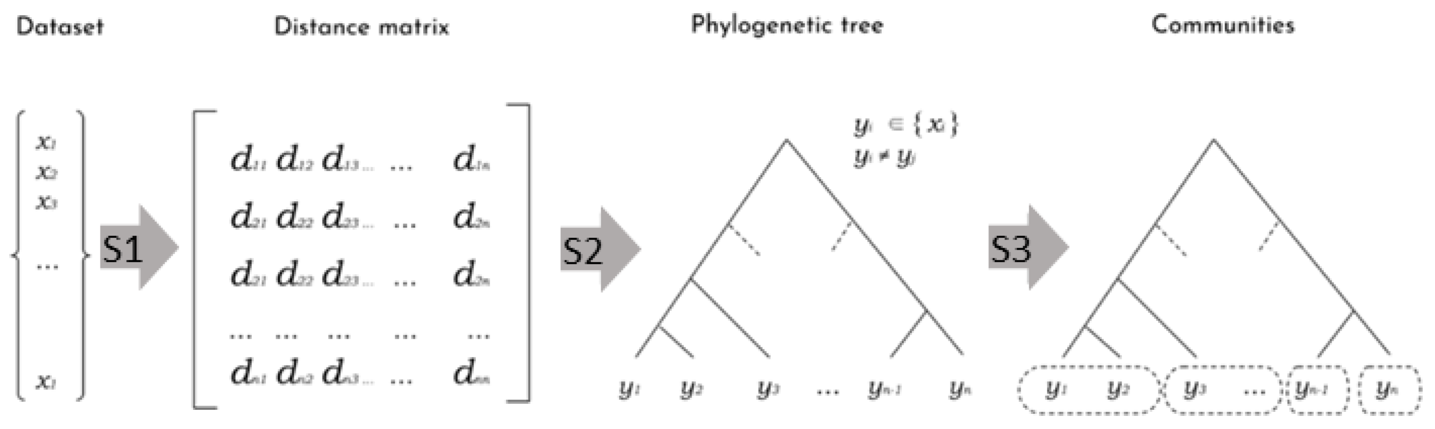
The foundations of FS-OPA are based on two methodologies that deal with large-scale and multidimensional data of any type, named DAMICORE [17] and FS-OPA [18]. The latter is a pipeline involving methods from Information Theory, Complex Networks, and Phylogenetic Inference, aiming at revealing hidden relationships of objects from an unstructured (raw) dataset. It runs in three main Steps: (S1) given a metric of similarity, build a distance matrix comparing every two objects; (S2) convert the matrix into a phylogenetic tree by connecting close objects according to hierarchical levels of similarity; (S3) apply a community detection process to group near subtrees into clusters. Figure 1 shows a set of generic objects x_i. The elements d_ij of the distance matrix correspond to a measure of dissimilarities between objects xi and x_j, according to some given metric. The matrix is broken down into a tree, where the distance between any two objects (leaves) corresponds to the sum of the lengths of the branches connecting them. Finally, the third step merges objects strongly connected (according to the tree topology) into a community, generating a set of different similarity clusters.

The first implementation of DAMICORE used three specific algorithms for S1, S2, and S3 (Figure 1), respectively, Normalized Compression Distance (NCD) [19], as it works with for any data type and mixed types; Neighbor-Joining (NJ) [20], widely employed in bioinformatics; and Fast Newman (FN) [21], that constructs a graph partition using a greedy algorithm based on a bottom-up strategy for maximizing the graph modularity function [22]. The pipeline with NCD, NJ, and FN possesses some distinctive properties. NCD makes DAMICORE a data-type agnostic method; in the sense that it works with any object (continuous, discrete, categorical-ordinal, and nominal variables, texts, images, audio, etc.) and a mixture of data types.

DAMICORE has some properties that make it proper for dealing with problems with a low level of previous knowledge, carried out by non-experts, or that would require a large multidisciplinary team of experts. First, it can run without any data pre-processing (such as filtering, outlier detection, feature extraction, parameter setup, and knowledge of the problem domain). Second, it requires no parameters setup to run and is therefore not biased toward arbitrary tuning constants. Naturally, pre-processing steps and some execution options may improve the DAMICORE performance. Its success in such a challenge has been checked for problems in a variety of fields, such as software-hardware co-design [23,24,25], compiler optimization [26], student profiling in e-learning environments [27,28], identification of phytopathology from sensor data [29], systematic literature review, identification of cross-cut concerns [30], and electrical distribution systems [31].

A Feature Sensitivity (FS) analysis aims to make salient the principal features of a problem (that may differ from selecting the main components), facing common challenges in some classes of real-world problems. For example, the quality of observed data, the database consistency and representativeness, and the discovery of interactions between features and their contributions to each target or objective are hard to check from a raw dataset with low previous domain knowledge. Thus, such a scope differs from those where the standard feature selection algorithms have usually succeeded. Moreover, an FS strategy is expected to aid in learning the fundamental structures of a complex problem from scratch. The learned structures can induce a probabilistic model used by optimization algorithms, such as in the Estimation of Distribution Algorithms [32]. In this research, we use phylogram-based models since they can work with small datasets, they are computationally efficient, and there is an optimization approach designed to use such models: Optimization based on Phylogram Analysis (OPA).

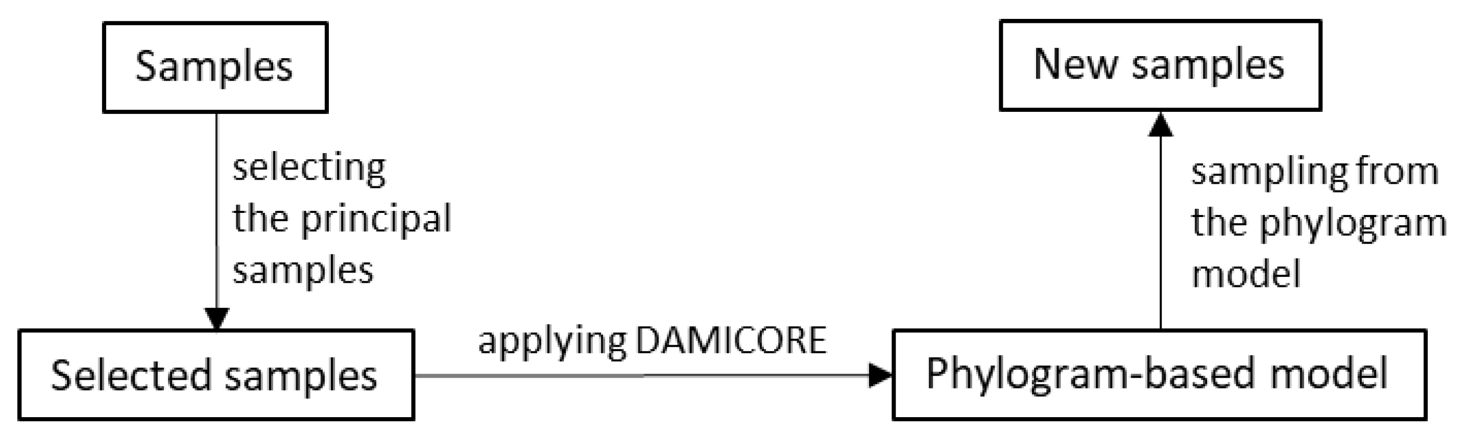
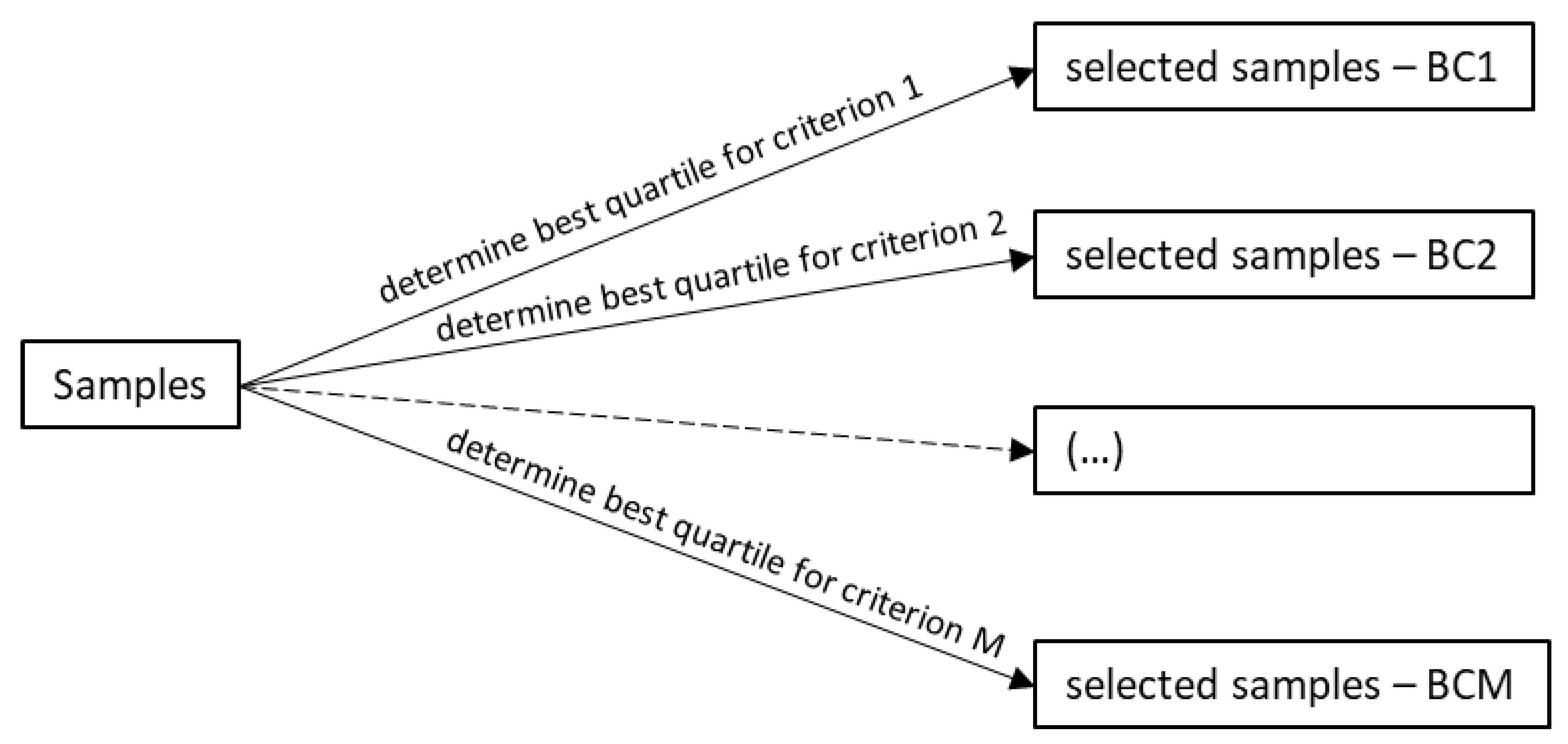
Figure 2 shows a diagram summarizing OPA and its use of the FS analysis. Such a combination is called FS-OPA. The two main FS steps are (A) "Salienting Samples (SS) according to a criterion" and (B) applying DAMICORE to construct a phylogram-based model. SS ranks the samples according to each of the M criteria (or non-dominated fronts), producing the sets of selected samples (Figure 3), denoted BC1 (the samples in the best quantile according to Criterion 1), BC2, …, BCM. DAMICORE constructs a phylogram (a rough model) from BCi, i = 1, …, M, generating M models (BC1-based model, …, BCM-based model). Then, a consensus strategy produces a unified phylogram-based model. An OPA cycle completes when the unified model generates new samples.

OPA performance has been verified for relatively complex combinatorial mono- and multi-objective optimization problems [32]. Basic proofs concerning (stochastic) convergence to optima and time–space complexity have been provided [32,33].

2.3. Comparison of FS-OPA with NL-MVU-PCA for MaOPs Data-Driven Structural Learning

NL-MVU-PCA is the primary method used by Duro et al. [12] for finding the essential objective set in MaOPs. Such a scheme also runs PCA based on the objective–function correlation matrix, aiming to improve objectives’ preference ranking. On the other hand, NL-MVU-PCA maximizes the variance in objective space while preserving the local isometry (common property in dimensionality reduction through embedding’s). NL-MVU-PCA is computationally more complex than PCA since the former solves an optimization problem. The non-linear (NL) approach performs the optimization of the Kernel (Gram) matrix values by minimizing the Maximum Variance Unfolding (MVU) to find the best mapping that preserves the geometric properties of each neighbourhood.

Table 1. NL-MVU-PCA and FS-OPA for multidimensional data-driven structural learning applied to real-world MaOPs.

Category	Types		NL-MVU-PCA	FS-OPA
Analyses	Objective-objective		X	X
	Variable-variable			X
	Variable-objective			X
	Objective space reduction		X
	Sensitivity			X
Priors	Kernel function usage		X	Not necessary
	Parameter optimization		X #	Not necessary
Variable and objective representation	Continuous		X	X
	Discrete (integers, real intervals)		X	X
	Ordinal		X	X
	Nominal		X	X
	Mixed			X
Explainability	Implicit		X
	Explicit (The Why)			X
User-friendliness	Stakeholders can easily run FS-OPA and understand results even for a large number of variables and/or objectives			X
Scalability	Time-complexity	Usual cases	O(M3q3) *	O(l3) **
		The worst case	O(M6)	O(nl2 + l3)
	Sample-size support		Empirical	Theoretical and empirical

* M is the number of objectives, and q is the number of clusters; ** l is the number of variables and objectives, and n is the number of data resamples; ^# Reference [5] shows that one can avoid parameter optimization for a new problem by choosing q = M − 1 for NL-MVU-PCA.

synthesizes some relevant properties of NL-MVU-PCA and FS-OPA for MaOPs. The latter analyses three types of associations: variable-variable (producing results similar to the Gibbs measure for Ising Models or Markov Random fields [34]), objective–objective (the dissimilarities, when found, can favour the construction of (non-dominated) front distributions [35]), and the variable–objective (that may benefit inference as Markov Blankets [36]). The former works on the objective space for space reduction to determine the essential objective set [12]. FS-OPA also has other properties that are relevant for some classes of real-world problems: (i) it preserves the original variable space, which favours non-experts interpretability; (ii) it works with any data type (continuous, discrete, categorical—not only ordinal, but also nominal data, addressed by Bandaru et al. [4]) and mixed types (proper for multiple heterogeneous databases with observed data); (iii) it has a relatively low time complexity; (iv) and, finally, it has generated applicable models when applied to learn from small datasets [17,23,24,25,26,27,28,29,30,31].

Reference [5] shows the use of NL-MVU-PCA for a mixed-variable problem, the gearbox problem (with continuous and discrete variables and continuous objectives). NL-MVU-PCA works on the (continuous) objective vectors for the gearbox problem. It differs from the meaning of mixed in Table 1, which relates to both the variable and objective representation (important for the "explicit explainability"), i.e., the mixture may include data vectors simultaneously from both spaces with different types. Moreover, FS-OPA can naturally work with any number of combinations of data types due to its foundation on NCD.

Concerning Explainability, "Explicit" means to provide a knowledge representation (with clues for "The Why" as the potential influence of variables on objectives) that benefits decision-maker interaction, while "Implicit" refers to the capacity to reveal the objectives’ relative importance for an optimization problem, e.g., by ranking them.

The Feature Sensitivity (FS) analysis of FS-OPA aims at finding the variable and/or objective data-driven interactions to construct structural (graph-based) and probabilistic modelling. Probabilistic results are fundamental when dealing with the odds of bias in observed data or small-data sampling. Explainability is also essential for some classes of real-world problems, mainly those concerning decisions by stakeholders. Moreover, a user-friendly tool (instantiating the FS-OPA methodology) is relevant for real-world applications involving practitioners or stakeholders who are not optimization or artificial intelligence experts. Variable–variable and variable–objective interactions can also benefit practitioners’ comprehension (The Why), increasing their confidence. Finally, the phylogram-based representation of those interactions has scaled up the understanding of results for some problems with dozens of variables or objectives (note that the interactive data mining approach proposed by Bandaru et al. [4] works with two or three objectives).

Table 1 also shows the time complexity for usual cases and the worst case to estimate the overhead of both procedures. The number of clusters in NL-MVU-PCA relates to the number of constraints to maintain the local isometry (M q; but in the worst case q = M − 1, resulting in M2) [12]. FS-OPA with usual resampling is O(l³) since n ⩽ l (as in leave-one-out resampling) [34]. Moreover, l = M in a space analysis only uses objectives. Thus, the time complexities of FS-OPA and NL-MVU-PCA have a ratio (n + M)/M⁴ (l/q³) of running time for l = M in the worst case (in the usual case).

Another relevant factor is the minimal samples required to ensure reliable findings. Usually, the sample size for the PCA-based approach is empirically determined. FS-OPA has a theoretical model to decide the minimal amount of samples that guarantees high confidence in the results, which has been empirically corroborated for relatively complex problems in the decision space of binary variables [32].

2.4. FS-OPA Framework

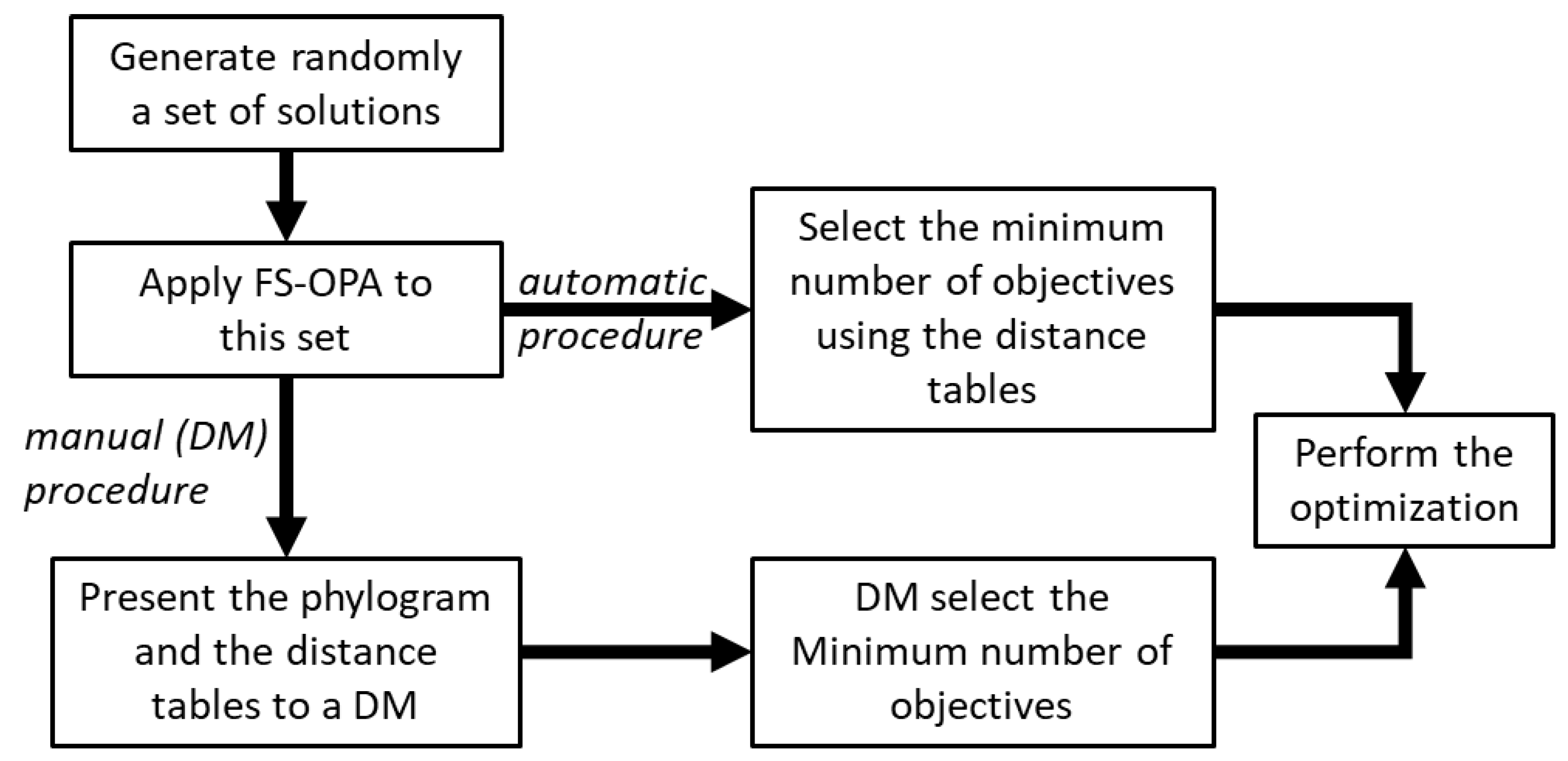
Figure 4 shows a flowchart of the global procedure of FS-OPA to reduce the number of objectives. Two options exist (i) automatic procedure, and (ii) procedure with the intervention of the DM(s). In the first case, the selection of the number of objectives to be used in the optimization is defined by the program automatically, using the table of the distance between objectives and applying the following rules:

• choose the objective(s) of the less distant clusters;
• choose one objective of the more distant (single) cluster;
• choose one objective from each of the remaining clusters.

In the second case, the selection is made by the DM(s), using both the phylogram and the table with the distance of objectives–objectives, as follows:

• choose the objective(s) of the less distant clusters;
• choose one objective of the more distant (single) cluster;
• choose objective(s) from each of the remaining clusters taking into account, also, the phylogram and the knowledge of the DM(s) about the process.

The reasons for rules 1 and 2 are different: the less distant cluster is the one that transports more information concerning the entire process, since it is near most of the decision variables, while the more distant cluster, besides everything, also has some information about the process that cannot be lost. The idea is that the intermediate clusters, selected by rule 3, have some information regarding the process that is already present in the objectives selected by rules 1 and 2, and thus, the objectives that can be discarded are those that belong to these clusters.

Both cases will be illustrated in the next section using a practical example. However, there are advantages and disadvantages to using one or the other. The first procedure provides the final solution directly, but the DM(s) does not take part in the process, which can imply some discomfort and distrust with the solution found. This does not happen when, after the analysis of the initial population of solutions, the DM(s) is confronted with relevant information about the process and, given these intermediate results, is asked about a possible way to advance. We are facing a situation in which the results may be explainable to the DM(s).

3. Examples of Application: DTLZ Benchmark Problems

A strategy to deal with many-objective real-world complex optimization problems (e.g., those with no explicit objective functions) is prioritizing objectives. In the case of unknown priorities, their relative importance can be estimated from samples of the decision space, as proposed in this paper. Such prioritization has a certain resemblance to the problem of determining the essential objective set, since a redundant objective has low priority.

The DTLZ problems (with and without redundant objectives) have been used to test the method’s capacity to find such a set and to evaluate algorithms for many-objective optimization.

Some algorithms have succeeded in finding the set from samples in POF, near POF, or, for example, from the last generation of an NSGAII run, although more recently, some of them failed for new challenging problems with other types of redundancies, as shown in [37]. This way, evaluating how much FS-OPA can estimate objectives’ relevance for DTLZs from a random population (or from the first fronts of it) may be useful, since they are well-known problems.

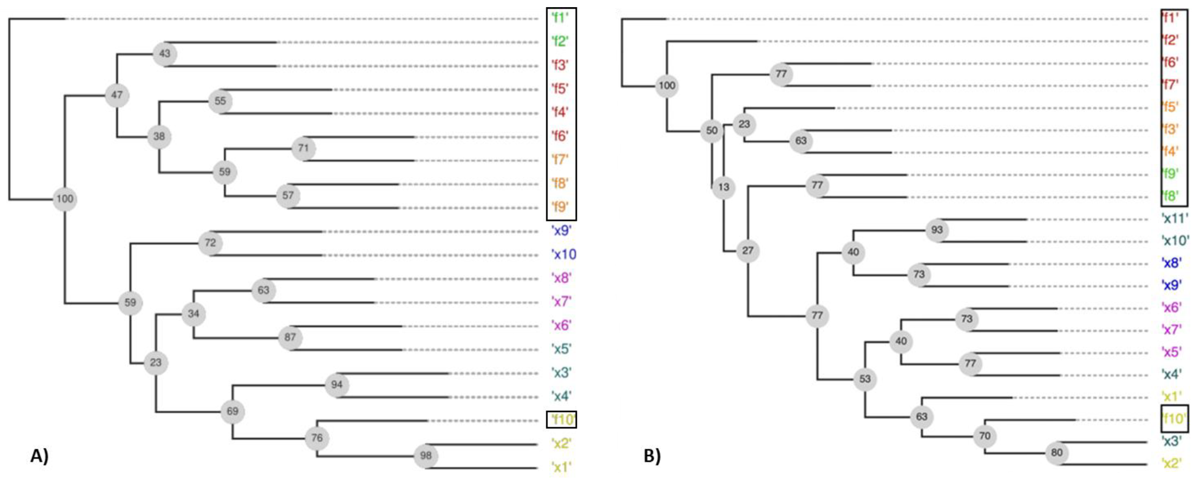
Figure 5A illustrates an FS-OPA output for unconstrained DTLZ5, also used by Duro et al. [12] for explaining the capacity of their method to find redundant objectives (objectives f₁, f₂, f₃, f₄, f₅, f₆, f₇, f₈, and f₉ are linearly correlated in DTLZ5). A random population of size 31 with samples normalized and Euclidian distance was used to obtain a distance matrix. SS procedure in Figure 3 was not applied. The output of Figure 5A shows variables and objectives arranged into a phylogram with leaf nodes (the objects under analysis) composing clusters (similarly to the end of the pipeline in Figure 1)—they are identified by the same color.

Objective functions f₁, …, f₉ are partitioned into three neighbor clusters ({f₁, f₂}, {f₃, f₄, f₅, f₆}, and {f₇, f₈, f₉}) in the phylogram structure; while f₁₀ is together with the leaf nodes, corresponding to variables. The phylogram structure aggregates f₁, …, and f₉ into the same subtree, while f₁₀ is isolated from the other objectives in the complementary subtree. The unique node with the label "100" (another type of result from a tree consensus) splits the phylogram into those two subtrees. Such a label (“100”) means that the leaf nodes f₁₀ and x₁, ..., x₁₀, and f₁₀ were in the same subtree (with the remaining leaf nodes in the complementary subtree) in 100% of all the constructed phylograms, independently of each subtree topology in a phylogram. Such an interpretation suggests a hypothesis: f₁₀ is weakly correlated to the other objectives, which are significantly associated with themselves. Thus, f₁₀ and one of the other objectives could compose an essential objective set; this result is consistent with the DTLZ5 problem structure.

Figure 5B shows the proposed phylogram for DTLZ5(2,10) with constraints (Saxena et al. [5]). It requires an additional variable, x₁₁, to generate samples outside POF, as samples used to construct a phylogram from Figure 5A. The phylogram from Figure 5B shows that f₁₀ is isolated in a subtree, while f₁, …, f₉ are in the complementary subtrees. Such a result suggests that f₁₀ and f₁ (for example) would enable proper POF estimates; this result agrees with the DTLZ5(2,10) problem structure.

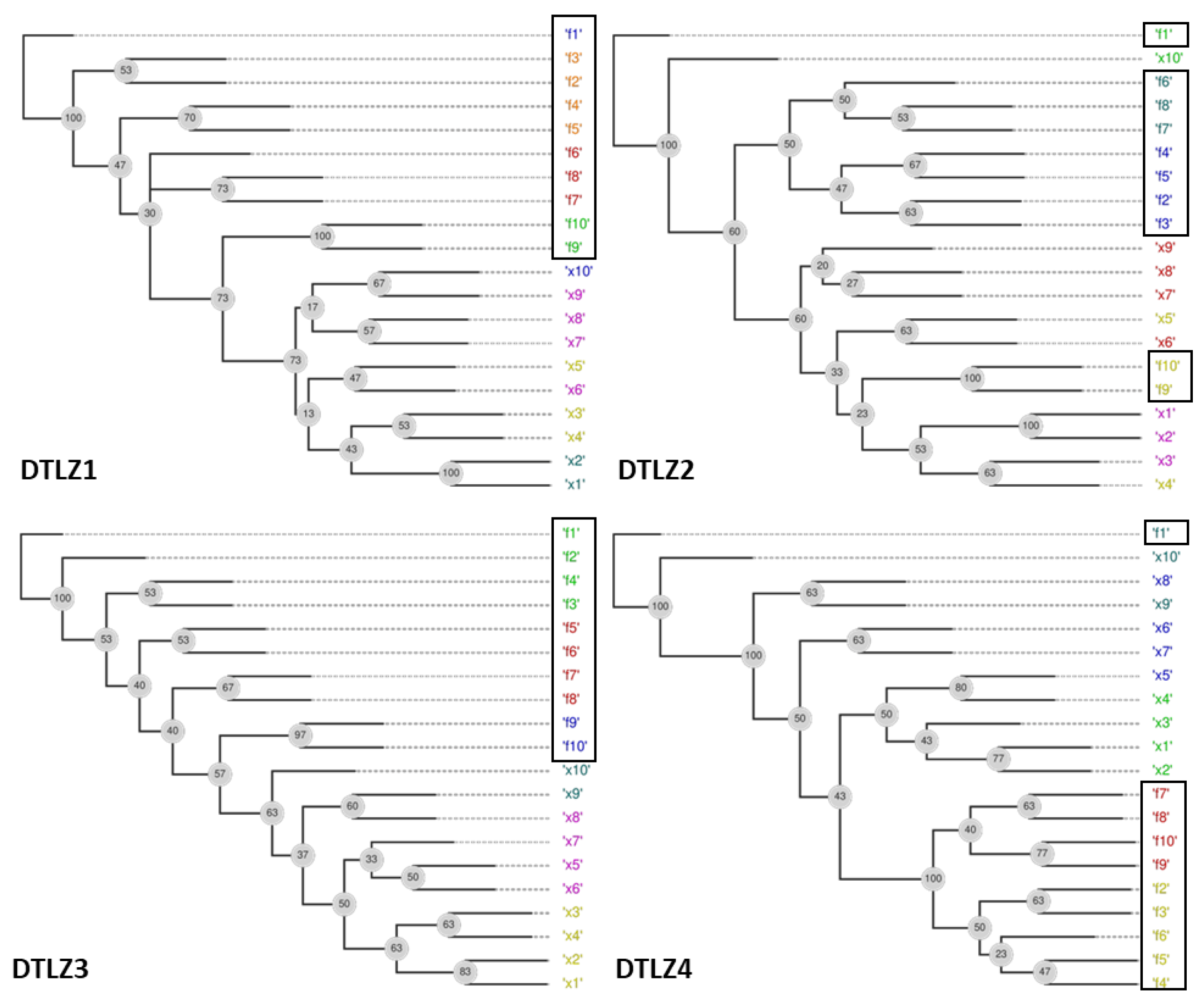
Figure 6 shows the phylograms obtained by FS-OPA for DTLZs 1–4 obtained from random populations of size 31 as a way to check if the FS-OPA clues about the objective relationships are plausible.

Given that these problems do not have redundant objectives, the unique possibility is to present some clue about the prioritization of objectives, considering that a reduction in the number of objectives only can be made with a certain error, as explained before. For example, the behaviours of functions DTLZ1, DTLZ2, and DTLZ3 are very similar. The simultaneous analysis of the clusters found and of the distances between objectives and the decision variables show that objectives can be portioned in the following sets:

• DTLZ1: {f₁}, {f₂, f₃, f₄, f₅}, {f₆, f₇, f₈}, {f₉} and {f₁₀};
• DTLZ2: {f₁}, {f₂, f₃, f₄, f₅}, {f₆, f₇, f₈}, {f₉} and {f₁₀};
• DTLZ3: {f₁}, {f₂, f₃, f₄}, {f₅, f₆, f₇, f₈}, {f₉} and {f₁₀};
• DTLZ4: {f₁}, {f₂, f₃, f₄}, {f₅, f₆} and {f₇, f₈, f₉, f₁₀};

This signifies that a possible hierarchization of the objectives for these problems can be made by selecting, in the first step, a single objective of the groups identified above and then, by selecting all the others to a second level.

In addition, all the objectives in the phylograms found for DTLZ2 and DTLZ4 are not in a subtree without a variable. That may mean that the disagreement of objectives of those two problems is more salient from an initial random sampling.

However, the objective of this paper is not only to define the minimum number of objectives that can be used without error but also to identify the situations where the reduction can be done with a certain error. Anyway, a deep analysis will be necessary here, which is outside of the scope of the present paper.

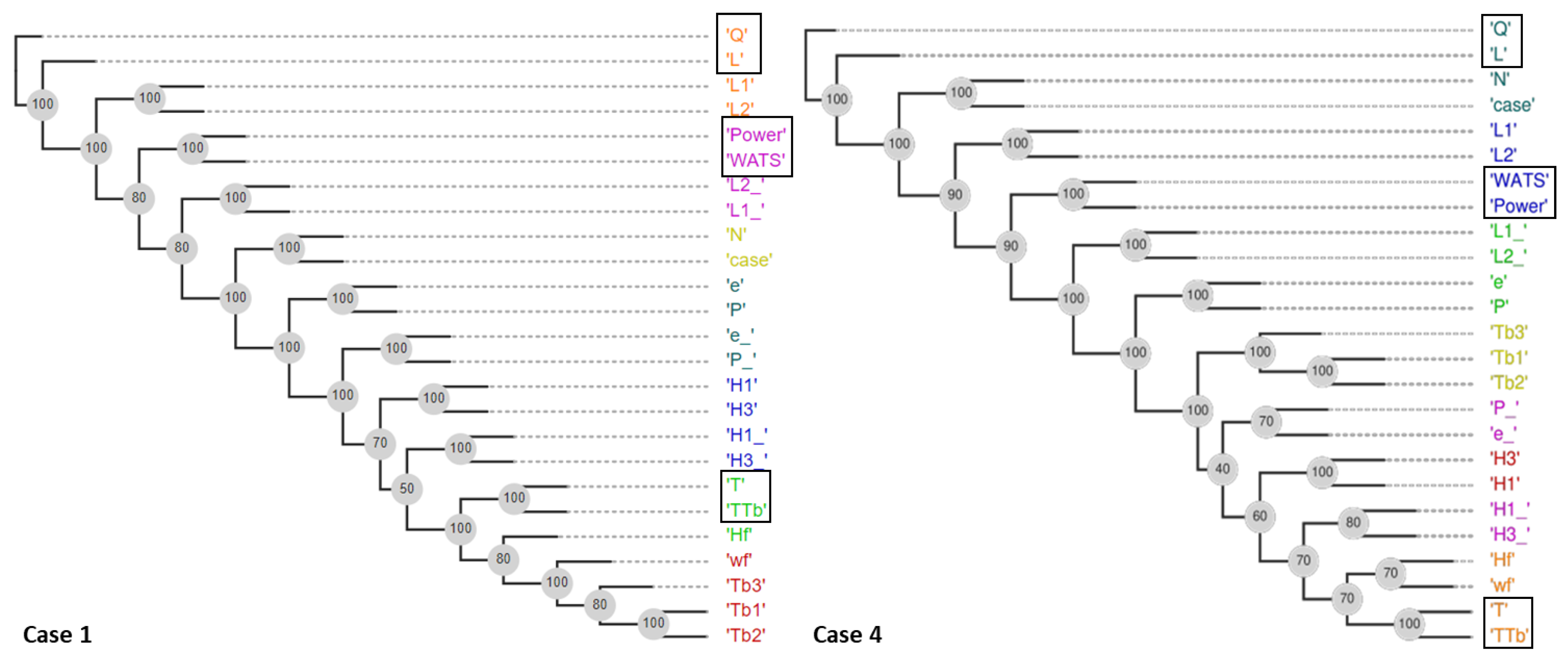
The FS-OPA also produces other outputs (useful for human comprehension of some classes of real-world problems), which are explored in Sections related to the extrusion problem.

4. Polymer Extrusion Problem

4.1. The Problem to Solve

To demonstrate the complexity of this system regarding the modelling program and the interrelations between the decision variables and the objectives, some details are given here. However, the system is much more complex, as can be seen in the following references [38,39,40,41].

Figure 7A shows an axial cut of the extruder and die fitted with a barrier screw. The sequence of the physical phenomena developing typically along the screw is also represented, and comprises [38,39,40]: (i) gravity conveying of the solid material in the hopper; (ii) drag solids conveying in the first screw turns; (iii) development of a thin film of melted material separating the solids from the surrounding metallic walls; (iv) melting of the solid plug, with physical separation of the solid plug from the melt pool; (v) melt conveying following a relatively complex regular helical flow pattern; vi) pressure flow through the die. Figure 7B shows the complex flow pattern quantified by the velocity fields and the temperature profile in the Conventional Screw (CS) and Maillefer Barrier Screw (MBS), while Figure 7C shows the complete system geometry used in the calculations.

The aim is to determine if the best solution is to use a CS or an MBS for fixed and/or for changing operating conditions and, simultaneously, to optimize the corresponding geometry.

The following equations represent the momentum and energy equations for the melted region of the channel (melting and melt conveying in Figure 7), which resulted from some specific simplifications of the general tri-dimensional (3D) set of equations. These equations were solved numerically, considering a 2D space representing the cross-screw channel (X and Y directions) for small increments along the channel (Z direction). However, it is necessary to note that all the regions identified above and in Figure 7 have different thermomechanical models that must be put together using the appropriate boundary conditions. This is a very complex system in which the polymer properties, the operating conditions of the machine, and the screw geometry contribute in a complex way to measure the process performance quantified by the objectives (see

Table 2. Optimization objectives, aim of optimization and range of variation.

Objectives	Aim	xmin	xmax
Output—Q (kg/hr)	Maximize	1	20
Length for melting—L (m)	Minimize	0.1	0.9
Melt temperature—T (°C)	Minimize	150	210
Power consumption—Power (W)	Minimize	0	9200
WATS	Maximize	0	1300
Viscous dissipation—Viscous	Minimize	0.9	1.2

).

For example, to only illustrate the complexity of this process and the corresponding numerical modelling, Equation (3) shows the melt rate per unit of channel length (Φ) that represents the quantification of solids material that changes the physical state to melt in each of the increments along the screw channel. However, we must take into account that it is an analytical model that resulted from further simplifications of Equations (1) and (2). For more details of the model used, the reader is referred to references [41,42,43].

$$\frac{\partial P}{\partial z}=\frac{\partial }{\partial y}\left(\eta \frac{\partial V_z}{\partial x}\right)+\frac{\partial }{\partial y}\left(\eta \frac{\partial V_z}{\partial y}\right)$$

(1)

$${\rho }_m{C}_s{V}_z(y)\frac{\partial T}{\partial z}=k_m\left(\frac{{\partial }^{2}T}{\partial x^2}+\frac{{\partial }^{2}T}{\partial y^2}\right)+\eta {\dot{\gamma }}^2$$

(2)

$$\Phi ={\left(\left\{\frac{V_{bx}{\rho }_m\left[k_m\left(T_b-T_m\right)+\frac{\eta }{2}{V}_j^2\right]}{2\left[C_s\left(T_m-T_{s0}\right)+C_m\left(T_{avg}-T_m\right)+h\right]}\right\}\right)}^{\raisebox{1ex}{$1$}\!\left/ \!\raisebox{-1ex}{$2$}\right.}$$

(3)

The variables in these equations represent the polymer properties, operating conditions and flow variables: ρ_m is the melt density, k_m is the melt thermal conductivity, h is the melting entropy, C_m and C_s are specific heat of melt and solids, respectively, T_m is the melting temperature, η is the melt viscosity, T_so and T_c are the solids and the barrel temperatures, $\dot{\gamma }$ is the shear rate, T is the melt temperature in each node of the mesh, T_avg is the average temperature of the melt, V_z is the melt velocity in the Z direction, V_s is the solid velocity in the y direction, and V_bx is the barrel velocity in the X direction.

Therefore, the performance of the process depends on the polymer properties, machine operating conditions and geometry. In the present example, a Low-Density Polyethylene (LDPE) is used, and for the operating conditions, two situations are considered, as shown in

Table 3. Cases studied for LDPE—only in case 7 the operating are used as decision variables.

Case	Operating Conditions	Decision Variables
		N (rpm)	Tb1 (°C)	Tb2 (°C)	Tb3 (°C)	Geometry
1	Constant	40	140	150	160	Table 4
2	Constant	60	140	150	160	Table 4
3	Constant	80	140	150	160	Table 4
4	Variable	[40, 80]	[140, 160]	[150, 170]	[160, 200]	Table 4

, i.e., in some cases, they are fixed, and in one of the cases, they are also considered as a DVs. The DVs are the operating conditions and the geometrical parameters as identified in Table 3 and

Table 4. Geometrical parameters of both CS and MBS screws.

Screw Type	Decision Variables
CS	case	L1	L2	H1	H3	P	e
MBS		L1_	L2_	H1_	H3_	P_	e_	Hf	wf
Interval	[0, 1]	[100, 400]	[170, 400]	[18, 22]	[22, 26]	[25, 35]	[3, 4]	[0.1, 0.6]	[3, 4]

, respectively.

The performance of the machine was quantified using six objectives, two to maximize (output and degree of mixing) and four to minimize (length of screw required to melt the polymer, melt temperature at the exit, mechanical power consumption required to rotate the screw, and viscous dissipation quantified as the ratio between the melt temperature and the fixed barrel temperature), as shown in Table 2.

The geometrical parameters involved in the description of both types of screws are shown in Table 4. Since only one screw can be used each time in the machine, an additional decision variable was added, identified as “case,” to trigger the decision variables corresponding to one of the types of screws, i.e., when case ranges in the interval [0.0, 0.5] the decision variables of the conventional screw are used, while when case ranges in the interval [0.5, 1.0], the other screw is considered. Consequently, the total number of decision variables is 15.

For each case studied (Table 3), 11 optimization runs are made for statistical comparison using the hypervolume (HV) and the Inverted Generational Distance (IGD).

4.2. Results and Discussion

The FS-OPA analysis for Cases 1 and 4 are presented in Figure 8 and

Table 5. Distances between the objectives for Case 1.

	‘Q’	‘L’	‘T’	‘Power’	‘WATS’	‘TTb’	Average
‘Q’	0.00	0.07	0.73	0.27	0.27	0.73	0.345
‘L’	0.07	0.00	0.73	0.27	0.27	0.73	0.345
‘T’	0.73	0.73	0.00	0.67	0.67	0.07	0.478
‘Power’	0.27	0.27	0.67	0.00	0.07	0.67	0.325
‘WATS’	0.27	0.27	0.67	0.07	0.00	0.67	0.325
‘TTb’	0.73	0.73	0.07	0.67	0.67	0.00	0.478

and

Table 6. Distances between the objectives for Case 4.

	‘Q’	‘L’	‘T’	‘Power’	‘WATS’	‘TTb’	Average
‘Q’	0.00	0.08	1.00	0.42	0.42	1.00	0.480
‘L’	0.08	0.00	1.00	0.42	0.42	1.00	0.480
‘T’	1.00	1.00	0.00	0.83	0.83	0.08	0.620
‘Power’	0.42	0.42	0.83	0.00	0.08	0.83	0.430
‘WATS’	0.42	0.42	0.83	0.08	0.00	0.83	0.430
‘TTb’	1.00	1.00	0.08	0.83	0.83	0.00	0.620

. The results were very similar, generating the same three groups of objectives, (Q, L), (Power, WATS), and (T, TTb). The application of the methodology defined in Section 2.4 allows for identifying the objectives Q, Power, WATS, and T to be used in the optimization after reduction (see Table 5 and Table 6): (i) the objectives with lower distance. Power and WATS; (ii) one objective of the cluster with higher distance, T; and (iii) one objective of the remaining cluster, Q. It is clear, also, that instead of T, it is possible to select TTb, and instead of Q, it is possible to select L.

To assess the capacity of using only the four objectives selected, the optimization results obtained using SMS-EMOA provided with the problem with these four objectives will be compared with the case with the initial six objectives using the Pareto-optimal fronts obtained after 100 generations for a population of 100 individuals in each generation and 11 runs with different seeds values are made for statistical comparison. Additionally, this comparison will be made with a situation with three objectives one of each of the clusters found, specifically Q, WATS, and T.

Figure 9 and Figure 10 show the Pareto-optimal fronts found in each one of the cases (Case 1 and Case 2) using the three sets of objectives: (i) all objectives; (ii) objectives Q, Power, WATS, and T; (iii) objectives Q, WATS, and T. The results are, apparently, very similar when comparing the cases with six and four objectives. In the other situation, with three objectives, the multi-objective optimization algorithm is clearly lost, since the final solution found alternates in the different runs between one type of screw and the other (i.e., between the CS and the MBS). The results for Cases 2 and 3 are very similar to those presented here and, thus, no specific discussion is made here.

By using the 11 runs performed for each case studied, the Hypervolume (HV) and the Inverted Generational Distance (IGD) were applied and the results are presented in

Table 7. Performance comparison using Hypervolume and IGD for the total number of objectives and the automatic reduction to four and three objectives (between brackets the standard deviation, and loss percentage relative to six objectives) for the four cases studied.

Case Study	Metric	6 Objectives	4 Objectives (Q, Power, WATS, T)	3 Objectives (Q, WATS, T)
1	HV	0.21518 (0.008145)	0.19148 (0.012324) −11.0%	0.02555 (0.024707) −88.1%
	IGD	0.10966 (0.004972)	0.11159 (0.003607) −1.76%	0.66727 (0.143866) −508%
2	HV	0.23233 (0.013760)	0.20867 (0.010411) −10.2%	0.04689 (0.028991) −79.8%
	IGD	0.10966 (0.004972)	0.11205 (0.003526) −2.17%	0.69042 (0.105262) −529%
3	HV	0.24809 (0.006384)	0.21932 (0.014301) −11.6%	0.04598 (0.0285391) −81.5%
	IGD	0.11076 (0.005756)	0.11326 (0.006315) −2.25%	0.69042 (0.105262) −523%
4	HV	0.24809 (0.006384)	0.22911 (0.009955) −7.7%	0.01967 (0.011256) −92.1%
	IGD	0.11076 (0.005756)	0.11431 (0.007949) −3.21%	0.72078 (0.046369) −550%

, where it is possible to see the average and the percentage of losses when the number of objectives is reduced [42,43,44]. To calculate IGD, all Pareto-optimal solutions found in each run were put together in a pool and the non-dominated solutions of this pool were used for comparison.

As shown in Table 7, it is possible to conclude that the use of four objectives (Q, Power, WATS, and T) does not significantly deteriorate the final solutions found, the maximum difference found is 11.6%, which, for a process like the extrusion process, and taking into account a final population of 100 solutions, is not expressive. Additionally, the differences in the IGD value are too small, indicating that at least the solutions found for the case of four objectives are near the best solution found in the 11 runs. The results found for the situation with three objectives corroborate the results shown in Figure 9 and Figure 10.

Finally, it is important to point out that during this process, the DM(s) play an important role in the procedure. Indeed, they have some intervention when selecting the objectives. For example, it is necessary to opt for Q or L, two objectives from the same cluster having apparently the same importance in the process. In this case, an informed DM will make the option for Q because this objective is the output of the machine and is directly linked with the economic issue of the problem, while L is the length for melting that is related to the quality of the product obtained; however, this quality is also quantified by WATS, which was already selected by the algorithm. This example shows the importance of the DM(s) that simultaneously help the optimization process and are informed about the process of obtaining the results.

5. Conclusions

A methodology for reducing the number of objectives for many-objective optimization problems using population-based algorithms is proposed. This approach, based on machine learning, is an improvement over similar state-of-the-art methodologies; namely, it allows analysis of the relations variable–variable and variable–objective relations (and not only objective–objective), does not need kernel function choice and parameters optimization, allows for obtaining explainable solutions to assist the decision maker with interpreting the results, its time complexity is also low, and it supports theoretical and empirical sample sizes.

The approach showed its potential to reduce the number of objectives by capturing the complex relations between the different objectives with an additional possibility, which is to capture the objective-variable relations. This is done by applying the methodology to a set of benchmark and real-world problems. The comparison of the Pareto-optimal fronts obtained with another machine learning approach in the literature allows for the conclusion that its performance is very competitive, but with the great advantage of being much easier to use. Additionally, there is the possibility of strong interaction with the DM(s).

The application of the proposed approach to a difficult real-world problem has proven that it is automatically possible to reduce the number of objectives by losing only around ten percent of the Pareto-optimal frontier obtained, for the case of 100 individuals in the population. The use of a second possibility, which is to require the intervention of the decision maker during the process, e.g., when selecting the objectives to be considered in the optimization, can be very useful because the person interested can see how the process works and interpret the results obtained. Finally, an important characteristic of the method proposed is the capacity to explain the solutions found.