1. Introduction
American options are contracts allowing the holder to exercise the option to sell or to buy an asset at a certain price at any time prior to and including its maturity date. The pricing of American options plays an important role both in theory and in real derivative markets. The option pricing model developed by Black and Scholes [
1] and extended by Merton [
2] has given rise to a partial differential equation governing the value of an option. Schwartz [
3] and Brennan and Schwartz [
4,
5] were the first to apply a finite difference method to price American options. The accuracy of their finite difference method was proved by Jaillet et al. [
6]. Other papers present finite difference methods (see, for example, Hull and White [
7], Duffy [
8], Wilmott et al. [
9]). An alternative approach is based on front-tracking methods that keep track of the boundary and discretize the problem in changing domain; they have been considered in [
10,
11,
12].
When we price an American option, we also need to determine the optimal exercise moment as a function of the value of the underlying asset. This leads to the formulation of a free boundary of the non-linear problem for the price of the American option when looking for a boundary that changes over time to maturity, known as the optimal exercise boundary. In particular, the American call option problem is a free boundary problem defined on a finite domain. On the other hand, the American put option problem is a free boundary problem that is defined on a semi-infinite domain, meaning that it is a non-linear model complicated by a boundary condition at infinity. The difficulty associated with a free boundary problem can be solved by using a front-fixing method—an approach relying on a change of variable to map the changing domain into a fixed domain.
The front-fixing approach has been considered in several papers. Holmes and Yang [
13], used a front-fixing finite element method. Tangman et al. [
12] introduced a fourth-order accurate finite difference scheme. In [
14], the original problem was transformed into a more manageable equation with coefficients that are not dependent on the spatial variable, and an explicit update for the location of the free boundary at each time step was used; furthermore, in Zhu et al. [
15], the secant method was employed to solve the non-linear problem. Moreover, in Tangman et al. [
12,
15], the difference between the prices of American options and European options was computed. Sevčovič [
16] studied and approximated the early exercise boundary for a class of nonlinear Black–Scholes equations, applying a fixed-domain transformation and using an operator splitting iterative numerical technique. Lauko and Ševčovič [
17] introduced a local iterative numerical scheme and compared analytical and numerical solutions for the early exercise boundary position computation of the American put option. In [
18], Zhang and Zhu presented a predictor corrector method after the fixed-domain transformation. Nielsen et al. [
19] used both explicit and implicit schemes to solve the Black–Scholes model of American options, while Company et al. [
20] presented an explicit finite difference method for the free boundary value problem under logarithmic front-fixing transformation. In [
21,
22], Fazio proposed an a posteriori error estimator for the numerical solution to the American put option obtained by an explicit finite difference scheme.
In this paper, we present an implicit finite difference scheme combined with the use of the front-fixing method in order to solve the American put option problem without dividend payments. Preliminary results have been presented to the International Conference ICNAAM2015 [
23]. We use a front-fixing variable transformation to reformulate the variable domain problem into a non-linear problem on a fixed rectangular domain. For the non-linear problem, we introduce a suitable choice of a truncated boundary that allows us to impose the asymptotic boundary condition. Then, the original problem is transformed into a new non-linear partial differential equation where the free boundary appears as a new variable and is computed as part of the solution. We develop an implicit finite difference method and we investigate the consistency and the stability property by fixing the values of the free boundary and of its first derivative.
Finally, we choose to validate the obtained numerical results via a mesh refinement and a Richardson’s extrapolation technique, and we present a comparison with numerical results available in the literature.
3. The Front-Fixing Method
The front-fixing method is widely employed for solving free boundary problems. The basic idea of the front-fixing method is to use a variable transformation in order to remove the free boundary and then to transform the original equation into a new non-linear partial differential equation on a bounded domain, where the free boundary appears as a new unknown of the problem. The main advantage of the front-fixing method is that the free boundary is computed directly.
Then, we first transform the Black–Scholes equation into a new parabolic equation over a bounded domain, we introduce a truncated boundary, and then we define an implicit finite difference scheme for the new approximate problem over a bounded domain.
According to Wu and Kwok [
14], we consider the dimensionless new variables
it follows that
is mapped on the fixed line
,
and
. Then, the put option problem (
1) can be rewritten as follows:
on the domain defined by
and
.
In order to solve the obtained problem numerically (
3)–(
6), we have to consider a finite computational domain. Then, we introduce a truncated boundary value
, which is a suitably large value where it would be convenient to impose the asymptotic boundary condition. In other words, we replace the asymptotic boundary condition (
5) with the side condition
For the choice of
and the accuracy of the related numerical solution, we follow the approach of Kangro and Nicolaides [
24], which was used to solve the multidimensional Black–Scholes equation.
By setting an integer
J and a positive value
, we define the step-sizes
the integer
N
where
is the ceiling function that maps a real number to the least integer that is greater than or equal to that number. Therefore,
is the grid-ratio
Therefore, within the finite domain, we can introduce a mesh of grid-points
for
and
. We would like to define a numerical scheme that allows us to compute the grid values
for
,
and the free boundary values
for
.
4. A New Implicit Finite Difference Scheme
Here, we present the implicit finite difference scheme for (
3)–(
6), which to the best of our knowledge has never been used for this problem.
for
and
.
The initial conditions (4) are given by
for
. From the boundary conditions (
7), we get
for
.
Moreover, by considering the governing differential Equation (
3) at
,
and taking into account the side conditions (
6), one gets a new boundary condition
(see Wu and Kwok [
14], Zhang and Zhu [
18] or Kwok ([
25], p. 341)), and its central finite difference discretization
From the two boundary conditions (6), using a central finite difference formula at time
and considering (
10), we obtain
where
is a fictitious point out of the computational domain. Considering
and rearranging (
8), our implicit numerical scheme can be written as follows:
for
and
, where
Considering (
11) and putting
in (
12), we get
For
in (
12) we obtain
For
we have the equations
Then, at each time step, we obtain a system of
J equations, given by (
14)–(
17), in
J unknowns,
and
. The system (
14)–(
17) can be written in the following compact form:
where
, the coefficients matrix
has following form
and the mapping
is
The system (
18) can now be written as a non-linear problem in the form
The implicit discretization leads to the non-linear Equation (
19) for the price and the location of the free boundary at each time step.
6. A Posteriori Error Estimator
In this section, we describe the a posteriori error estimator for the American put options problem based on Richardson’s extrapolation. In this way, we can find a more suitable computational grid requiring that the numerical solution obtained by the implicit method verifies a prefixed error tolerance.
For a scalar
U of interest, either a value of the solution
or a free boundary value
, the numerical error
e can be defined by
where
u is the exact, usually unknown, value. When the numerical error is caused predominantly by the discretization error, in the case of smooth enough solutions, the global error can be split into a sum of powers of the inverse of
N
where
,
,
, ⋯ are coefficients that depend on
u and its derivatives but are independent of
N, and
,
,
, ⋯ are the true orders of the discretization error; see Schneider and Marchi [
27] and the references quoted therein. Each
is usually a positive integer with
which together constitute an arithmetic progression of ratio
. The value of
is called the asymptotic order or the order of accuracy of the method or of the numerical value
. By replacing
and
in Equation (
25) and subtracting into the second obtained equation the first times
, where
, we get the first extrapolation formula
which has a leading order of accuracy equal to
. This type of extrapolation is due to Richardson [
28,
29]. Taking into account Equation (
26), we can conclude that the error estimator using the first Richardson’s extrapolation is given by
where
is the order of the numerical method used to compute the numerical solutions. Thus, (
27) gives the real value of the numerical solution error without knowledge of the exact solution. In comparison with (
27), a safer error estimator can be defined by
Of course,
can be estimated with the formula
where
u is again the exact solution (or, if the exact solution is unknown, a reference solution computed with a suitable large value of
N) and both
u and
are evaluated at the same grid-points of
.
Within the above framework, in order to improve the numerical accuracy by using only a small number of grid-nodes, we can generalize (
26) by introducing the following repeated extrapolation formula:
where
,
,
is the grid refinement ratio, and
is the true order of the discretization error. Formula (
30) is asymptotically exact in the limit as
goes to infinity if we use uniform grids. We notice that, to obtain each value of
, we need two computed solutions
U in two adjacent grids, namely
and
g at the extrapolation level
k. For any
g, the level
represents the numerical solution of
U without any extrapolation. We recall that the theoretical orders of accuracy of the numerical values
, with
and
k extrapolations, verify the relation
valid for
.
7. Numerical Results
In this section, we show the numerical results obtained by using the implicit finite difference scheme. Comparisons with some numerical results available in the literature for the American put options problem are also presented. The numerical experiments were performed in MatLab on a computer equipped with a CPU Intel i7 under the operating system Windows 10.
The parameters considered for solving the American put option problem (
3)–(
6) are as follows:
In order to choose the truncated boundary value
, we compute the numerical solution
for three different values of
. As we can see in
Table 1, the change of these values does not greatly affect the numerical solution; for this reason, we decided to set
.
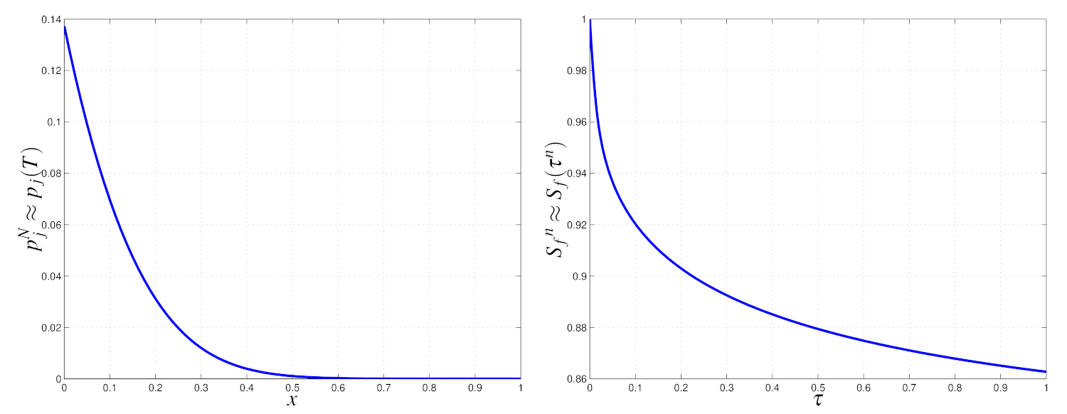
In
Figure 4, we show the plots of
versus
and of
versus
; these results were obtained by the implicit finite difference scheme, considering the parameters (
32) with
and
. We found the value
in
seconds. In order to solve the non-linear system, we used the MATLAB routine “fsolve”. In general, the Newton iterations method represents a good tool in order to guarantee good computational stability properties. Initially, we used the classical Newton iteration method, but the obtained numerical results were less accurate when compared with those obtained by the MATLAB routine
fsolve. By our numerical experiments, we conclude that the MATLAB routine, principally regarding the choice of the initial iterate, is more robust than the Newton iteration method and thus more suited for our application.
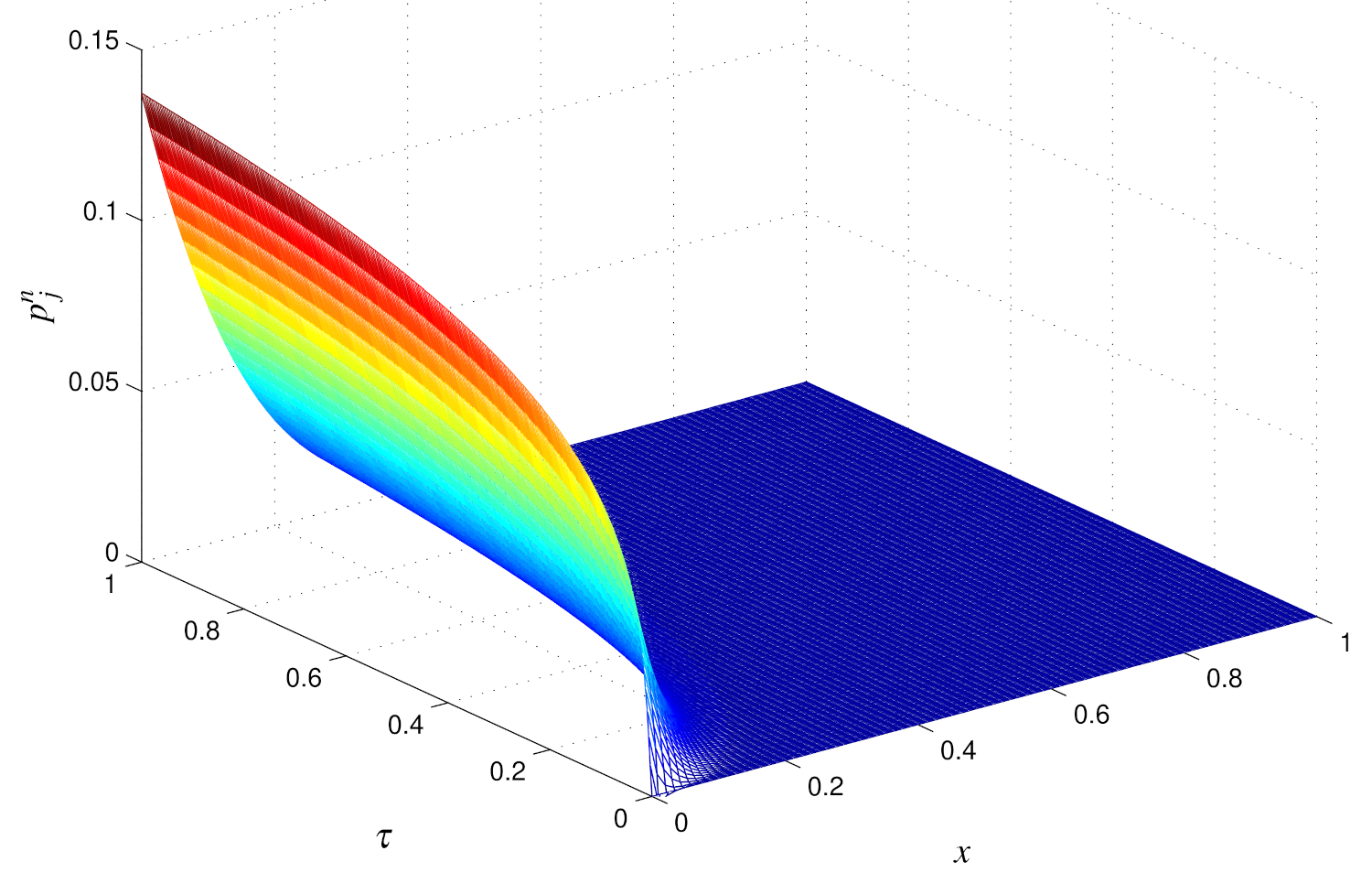
In
Figure 5, the 3D plot of the numerical solution
is shown.
Now, we consider the stability of the numerical method with respect to small perturbations of the starting parameters. In particular, we consider the perturbations
and
related to the parameters involved in the model, namely
r and
. In
Table 2, we show the numerical results obtained by different values of the perturbations. We can conclude that “small perturbations at input give rise to small perturbations at output”.
Looking at the results listed in
Table 1, we realize also that, when fixing a value of the truncated boundary
, the computed values of
for different values of the grid-steps are in agreement only up to the first decimal place. For this reason, we decide to improve the numerical accuracy by performing a mesh refinement and applying repeated Richardson’s extrapolation. The implicit difference scheme is accurate on the first order in time and second order in space; then, we can perform a mesh refinement keeping the grid ratio
constant so that we end up with second-order truncation error
in time. Therefore, the global error is of the first order, which is the value of
. In our case, the sequence of
, for
, with
and
is given by 4, 16, 64, 256, 1024, ⋯.
The numerical results obtained by repeated Richardson’s extrapolations for the values
computed with the implicit method are reported in
Table 3. The last extrapolated result is
, so we can consider this value as our benchmark
. Our result can be compared with the value
found by Fazio [
21], with
computed by Nielsen et al. [
19] and with
found by the explicit method of Company et al. [
20].
In
Table 4, we compare the option price
obtained by different methods with the following parameters:
We report the “true value” as in [
30], the penalty method (PM) of Nielsen et al. given in [
30], the explicit method (EM) of Company et al. [
20] with
, the explicit method with Richardson’s extrapolation (EMR) of Fazio [
21] with
and our implicit method (IM) without extrapolation, setting
and
, and with Richardson’s extrapolation (IMR) with
. In order to find the value of the option price
in correspondence to each different asset price
S we use a piecewise cubic spline interpolation.
Our goal was to solve the American put option problem with a given tolerance
, where 0 <
1; thus, we used the error estimator defined by Equation (
27), or alternatively by Equation (
28). To this end, we needed to solve the given problem twice, for two grids defined with given values of
and
of space intervals but for the same value of the grid-ratio
. The corresponding time intervals
and
verify the relation
. Thus, we were able to apply (component-wise) to
and to
the error estimator in Formula (
27) or (
28). Then, we could verify whether, for
,
If the two inequalities (
34) hold true, for
, then we can accept the numerical solution computed on the grid defined by
and
; otherwise, we have to increase these two integers and repeat the computation.
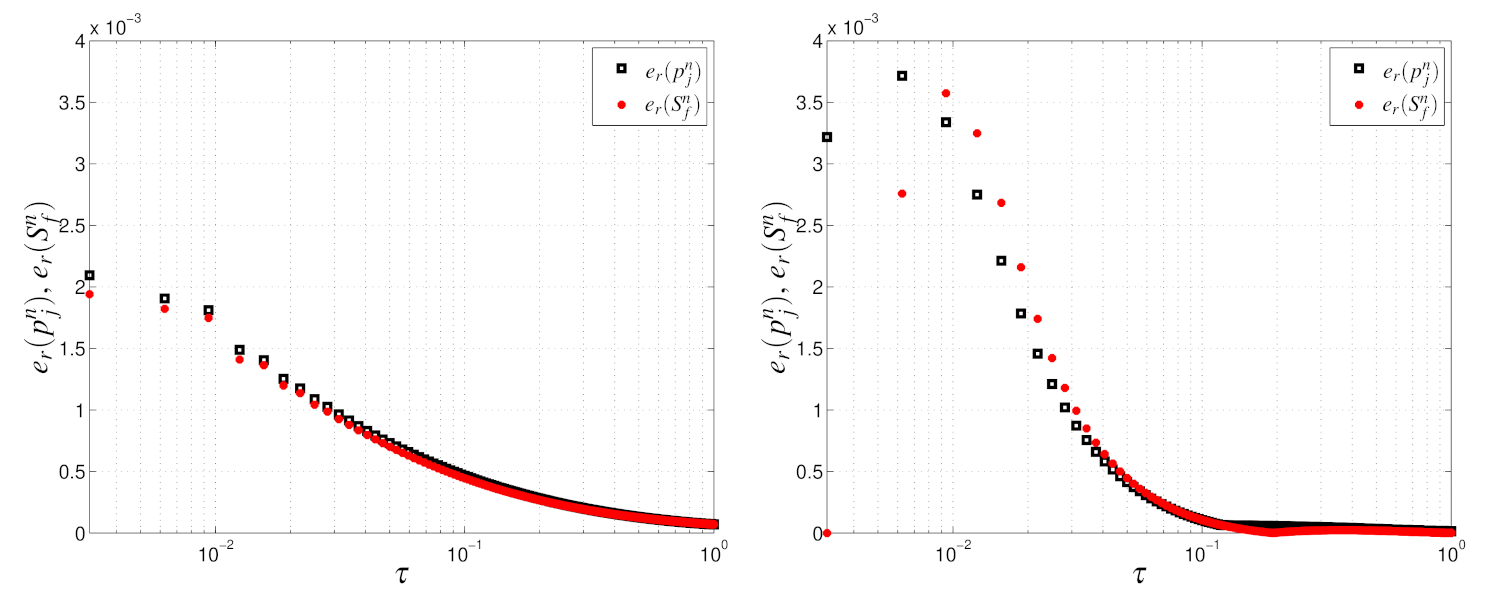
Figure 6 shows the error estimator results computed by setting
. We set
and start with
and
repeating the computation by doubling the number of spatial grid-intervals if the requi accuracy is not achieved. Our algorithm stops when
that for
means
.
From the numerical results shown in
Figure 6 we can easily see that the greatest errors are found within a few time steps for both numerical methods. The error of the implicit method is almost twice that of the error of the explicit scheme only in the first time steps, but it becomes smaller in the next time steps, so we can conclude that the numerical results obtained by the implicit method are more accurate than those of the explicit method. We suggest that in order to obtain better accuracy in the first time steps, an adaptive version of both finite difference schemes should be developed.


