Mechanism of Separation of Contaminants from Activated Carbon by Closed Cycle Temperature Swing Desorption

Abstract

In this paper, the mechanism of separation of volatile organic compounds (VOCs) from activated carbon adsorption beds during closed cycle temperature swing desorption was studied. Toluene gas at different concentrations was used as the gas for closed cycle temperature swing desorption to regenerate activated carbon beds saturated with toluene. This research advances our understanding of the separation of contaminants from activated carbon and the mechanism of the process by which waste gas with a background concentration desorbs activated carbon in hot gas with a background concentration, establishing a technological foundation for the closed cycle temperature swing desorption process of activated carbon. When the background concentration was 2 g/m³, the average desorption rates of unit activated carbon at 10 cm in 40 min and 60 min were the largest, at 0.0099 and 0.0067 g/ (g•min), respectively. The fit of the Bangham desorption rate equation was the best. When the background concentration of toluene was 2 g/m³ and the filling length of the activated carbon layer was 10 cm, the desorption rate constant was the highest, at 0.0152 min⁻¹.

1. Introduction

VOCs are widely produced, mainly from automobile exhaust emissions, industrial emissions, coal and biofuel combustion, diesel gasoline, or natural gas leakage and volatilization [1]. VOCs are one of the main reactants of near surface O₃. Some VOCs have active chemical properties, which may lead to the generation of photochemical smog and secondary pollutants after entering the atmosphere [2], causing serious harm to air quality and human production activities [3]. Commonly used VOC control technologies are mainly divided into destructive elimination methods and recovery methods [4,5]. Destructive elimination methods include biodegradation [6], incineration [7], catalytic oxidation [8], etc. Recovery methods include adsorption [9], absorption [10], condensation [11], etc. Adsorption is regarded as one of the most efficient ways to treat VOCs among these recovery methods. As a result of its high purification efficiency, flexibility, recyclable resources, low one-time investment cost and energy consumption, it is widely used in engineering projects [12].

The adsorption method includes the adsorption process for pollutants in waste gas, as well as the desorption and regeneration processes of activated carbon [13]. Activated carbon desorption reduces the force between the activated carbon and the adsorbate through the introduction of energy or substances, so that the molecules of the adsorbing components can obtain a certain amount of energy and then be desorbed from the solid surface [14]. Common temperature swing desorption methods include steam desorption regeneration and thermal nitrogen desorption regeneration. However, high energy consumption, poor safety and equipment corrosion are the downsides of traditional thermal regeneration technology [15]. The thermal nitrogen circulation–split flow condensation recovery process uses thermal nitrogen as the heat source for activated carbon desorption. The process has the advantages of high safety, an unlimited desorption temperature, a high desorption efficiency of activated carbon, and a high adsorption efficiency after regeneration [16]. Meanwhile, the waste emission and energy consumption of recycling desorption are low, which meets the requirements of a circular economy [17].

Previous research has demonstrated that when the desorption temperature is increased, the desorption rate considerably increases. Desorption with thermal nitrogen has a good regeneration performance [18]. Ethanol, ethyl acetate, cyclohexane and xylene were desorbed with activated carbon by temperature programmed desorption. At 160 °C, adsorbate molecules on activated carbon can be completely desorbed [19]. Chen et al. found that the regeneration efficiency could reach 87.09% after three cycles of regeneration when using I-TiO₂ photocatalysis to regenerate activated carbon saturated with toluene [16].

In this study, an experimental device was built to simulate the migration and diffusion of separation of contaminants from activated carbon by closed cycle temperature swing desorption. With toluene as the representative target contaminant of VOCs, the process conditions, such as the filling length of the activated carbon layer and the background concentration of toluene, were simulated by analyzing the evaluation factors such as the desorption outlet concentration, desorption amount, average desorption rate and instantaneous desorption rate. The concentration change of each activated carbon layer was continuously monitored during desorption to analyze the mass transfer kinetics of activated carbon by closed cycle temperature swing desorption. This research advances our understanding of the separation of contaminants from activated carbon, filling a gap in the understanding of the mechanism of the process by which waste gas with a background concentration desorbs activated carbon in hot gas with a background concentration, and establishing a technological foundation for the closed cycle temperature swing desorption process of activated carbon.

2. Materials and Methods

2.1. Adsorbent

In this experiment, 4.0 mm CTC90 granular activated carbon (GAC) from Ning Xia Hua Hui Activated Carbon Co., Ltd (Ningxia, China). was selected as the adsorbent.

Table 1. Characteristics of the GAC.

Adsorbent Name	Model	Diameter (mm)	Water Content (%)	Ash Content (%)	Strength (%)	Filling Density (g/L)	Carbon Tetrachloride Adsorption Value (%)
Granular Activated Carbon	CTC90	4	2.92	13.9	90.2	380	92.15

is a list of its physical and chemical characteristics.

2.2. Adsorbate

Toluene (analytically pure, content (GC) ≥ 99.5%) was selected as the representative adsorbate of VOCs.

Table 2. Physicochemical characteristics of toluene.

Adsorbate Name	Specifications	Content (%)	Molecular Formula	Boiling Point (°C)	Molecular Weight	Relative Density (kg/m3)
Toluene	Analytically pure	99.5	C7H8	110.6	92.14	865

is a list of its physicochemical characteristics.

2.3. Experimental Devices and Methods

The dynamic adsorption technique was used to measure the toluene adsorption equilibrium isotherms. Figure 1 depicts the experimental device. The adsorption saturated activated carbon was acquired by this device. At various temperatures and concentrations, the saturation adsorption capacities of toluene were measured. The inlet temperature and concentration of toluene were established 25–180 °C and 5–50 g/m³. The concentration of toluene gas adsorbed by activated carbon was 15 g/m³. The adsorption isotherms were measured using gravimetric techniques.

The experimental device took the ambient air of the laboratory as the air source, and the air was fed into the device by a blower. After the water vapor was removed in the silica gel drying device, it was divided into two paths according to the calculated proportion through the control of the digital display mass flowmeter. One way flow of gas entered the gas generation device with a set concentration, which was the carrier gas of toluene after volatilization, and entered the adsorption system after fully mixing with the dilution gas flowing the opposite way in the gas buffer chamber. In the adsorption system, the adsorption column was filled tightly and evenly with CTC90 activated carbon particles, and it was vertically placed into the constant temperature drying oven with the set experimental temperature using an iron frame. The mixed toluene gas first reached the experimental temperature through the gas preheating pipeline in the constant temperature drying oven, and then entered the adsorption column filled with activated carbon for the adsorption experiment. The adsorbed gas entered the detection system through the detection port, and the smart FID measured the outlet concentration of toluene through continuous sampling. When the inlet concentration generated by the gas generation device was consistent with the outlet concentration detected by the smart FID, the activated carbon in the adsorption column reached adsorption equilibrium.

Then, we used the desorption experimental device to carry out experiments and observed the separation of contaminants from the activated carbon layer. Figure 2 depicts the experimental device. Under condition of 0.2 m/s cross-sectional wind speed and 150 °C desorption temperature, the saturated activated carbon was desorbed by toluene gas at concentrations of 2, 5 and 10 g/m³. The activated carbon layer was 300 mm tall. The same loading method of the experimental device in Figure 1 was used to generate toluene gas of a certain concentration, and it was passed to the desorption unit in the constant temperature drying oven. Three columns of quartz glass, each measuring 10 cm in length and 4 cm in inner diameter, made up the desorption unit. The bottom of the quartz glass desorption column was filled with a 5 mm quartz sand layer to support the activated carbon and ensure the gas flow was even. The saturated activated carbon was desorbed for two hours under different working conditions, and each detection port was continuously monitored with a Smart FID. After the experiment, we used a balance to weigh the activated carbon after desorption.

The adsorption capacity of activated carbon was determined by the gravimetric method. Before and after the experiment, the activated carbon was weighed. Equation (1) was used to determine the adsorption capacity at the end of the adsorption phase:

$$x=\frac{m_2-m_1}{m_1}\times 100\%$$

(1)

where m₁ represents the mass of activated carbon prior to adsorption (g), m₂ represents the mass of activated carbon following adsorption (g) and x represents the adsorption capacity of activated carbon (g/g).

Before and after the experiment, the activated carbon was weighed. The integral method was used to draw the time curve of the desorption amount based on the time and toluene outlet concentration.

3. Results and Discussion

3.1. Adsorption Equilibrium Isotherm

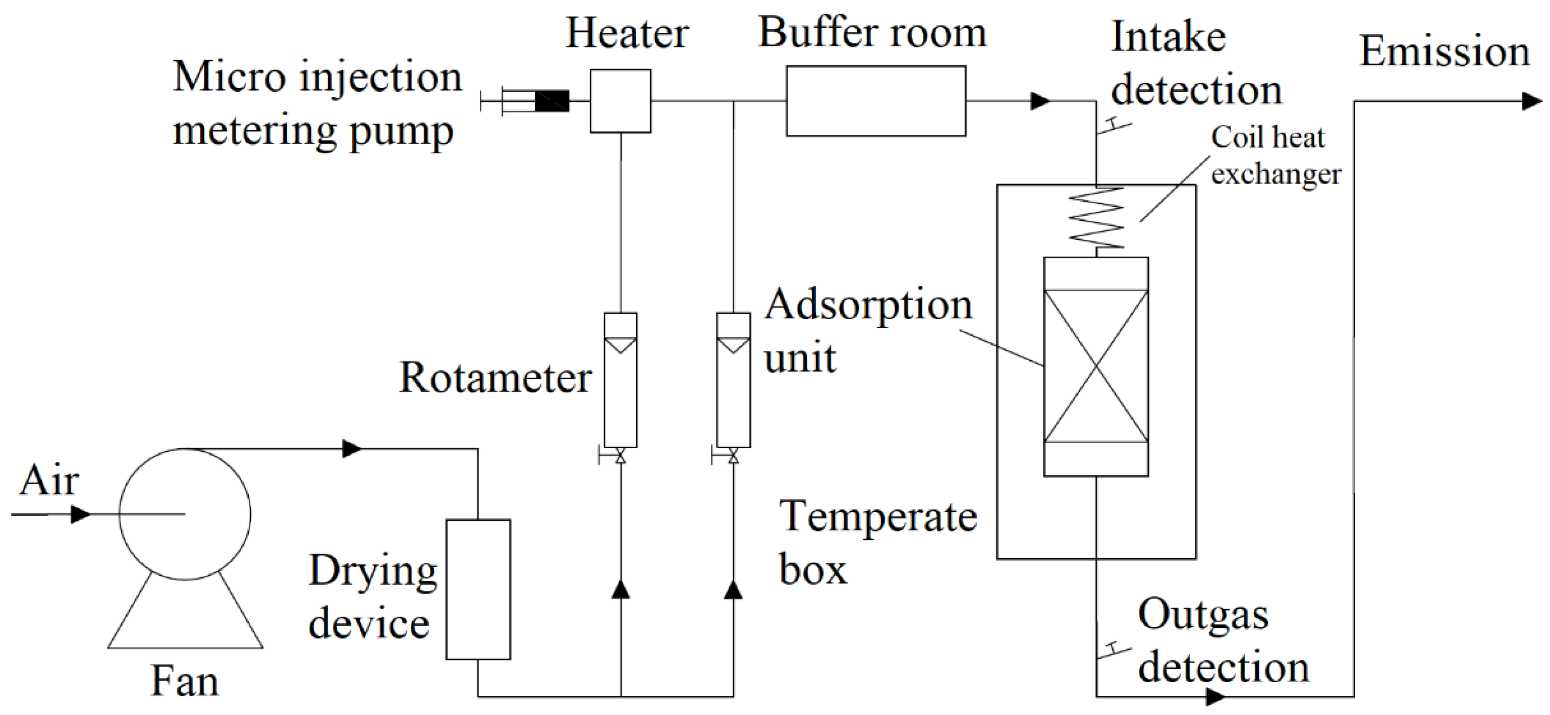
The foundation for our subsequent research was the isotherm of adsorption of toluene on activated carbon. We weighed the activated carbon bed before adsorption. At a particular temperature and concentration, the toluene gas passed through the activated carbon. We used a Smart FID to monitor the concentration of toluene gas prior to and following the stainless steel adsorber. We weighed the saturated activated carbon after the inlet concentration was stable and equal to the outlet concentration. The outlet concentration was used to draw the adsorption breakthrough curve. 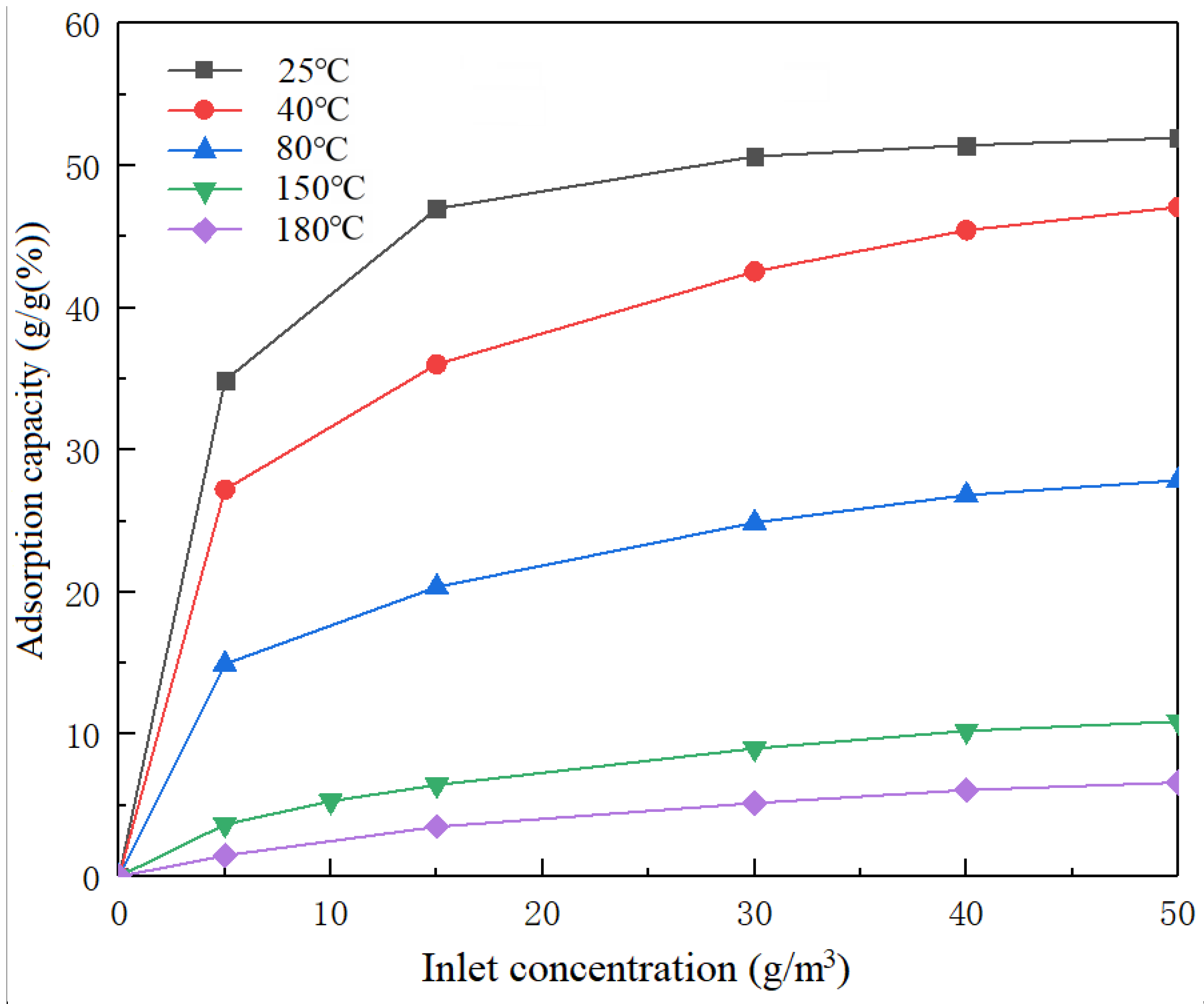Figure 3 illustrates the toluene adsorption isotherm curve for a range of experimental temperatures.

A type I adsorption isotherm of monolayer adsorption was suitable for the adsorption isotherm curve [20]. When the toluene concentration was 5 g/m³, the equilibrium adsorption capacity of CTC 90 for toluene at 25 °C was 0.349 g/g. The equilibrium adsorption capacities were 0.2720, 0.1490, 0.03650 and 0.01470 g/g at experimental temperatures of 40, 80, 150 and 180 °C, respectively. When the concentration of toluene was 50 g/m³, the equilibrium adsorption capacity at 25 °C was 0.5190 g/g. The equilibrium adsorption capacities were 0.4720, 0.2790, 0.1090 and 0.0660 g/g with experimental temperatures of 40, 80, 150 and 180 °C, respectively. The equilibrium adsorption capacity rose at the same temperature as the toluene concentration. When the toluene concentration was constant, the equilibrium adsorption capacity decreased with rising temperature. This was an exothermic reaction.

The curves in Figure 3 were well fit by the Freundlich and Langmuir adsorption isotherm equations. The adsorption isotherms of toluene at 25, 40, 80, 150 and 180 °C on CTC90 activated carbon were fitted. Figure 4 displays the results and the fitting curves. q_s in the Langmuir equation is the saturated adsorption capacity of a single molecular layer and q_s in

Table 3. Freundlich and Langmuir equation parameters of the adsorption isotherm curves.

Adsorbent	Temperature (°C)	Freundlich			Langmuir
		k (Pa−n)	n	R2	qs (g/g)	B (m³/g)	R2
CTC90	25	0.2848	6.1776	0.9898	0.5527	0.3494	0.9966
	40	0.1874	4.1884	0.9996	0.5020	0.2124	0.9530
	80	0.0973	3.6697	0.9993	0.3033	0.1704	0.9534
	150	0.0181	2.1533	0.9978	0.1455	0.0572	0.9905
	180	0.0068	1.6950	0.9939	0.1080	0.0315	0.9992

is close to the measured value of the adsorption isotherm experiment. B is the empirical adsorption equilibrium constant of the Langmuir equation. Its value indicates the adsorption capacity of gas molecules on the solid surface. The b value in Table 3 decreased with the rise in temperature, which was consistent with the conclusion that the equilibrium adsorption capacity decreased as temperature rose in the experiment. In the Freundlich equation, the constant k is related to the characteristics and temperature of the adsorbent and the adsorbate, and the constant n is related to temperature. Both can characterize the adsorption capacity of an adsorbent to an adsorbate, and these two parameter values also decrease with an increase in temperature. The R² of the Freundlich isotherm equation of activated carbon adsorbing toluene was basically higher than the Langmuir isotherm equation, and it was more stable, basically above 0.99. Therefore, with activated carbon adsorbing toluene, the Freundlich isotherm equation performed better than the Langmuir isotherm equation.

3.2. Working Capacity Curve

The equilibrium adsorption capacity was not zero when the desorption temperature reached equilibrium, so the maximum working capacity was used as the evaluation factor in practical applications. The working capacity was defined as the difference between the equilibrium adsorption capacity of an adsorbate of a certain concentration at a specific adsorption temperature and the equilibrium adsorption capacity of the corresponding equilibrium concentration when gaseous pollutants condense at a specific desorption temperature. The intake air concentration was taken as the abscissa and the working capacity as the ordinate. The adsorption temperature of activated carbon is 25 °C, and the desorption temperature is 150 °C. The working capacity under these working conditions was obtained by subtracting the equilibrium adsorption capacity corresponding to the toluene condensation temperature under the desorption temperature from the equilibrium adsorption capacity under each intake concentration. 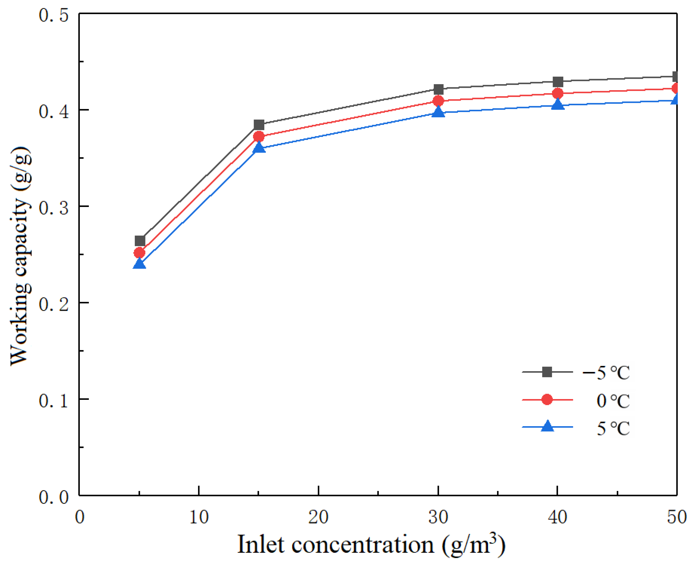Figure 5 shows the maximum working capacity curve of activated carbon to toluene at different concentrations under different inlet air concentrations.

When the inlet toluene concentration of the adsorption treatment gas was 5 g/m³ and the condensation temperatures of the circulating gas were −5, 0 and 5 °C, the working capacities of toluene were 0.2650, 0.2520 and 0.2400 g/g, respectively. When the inlet toluene concentration was 15 g/m³ and the condensation temperatures were −5, 0 and 5 °C, the working capacities of toluene were 0.3850, 0.3730 and 0.3600 g/g, respectively. When the inlet toluene concentration was 30 g/m³ and the condensation temperatures were −5, 0 and 5 °C, the working capacities of toluene were 0.4220, 0.4100 and 0.3970 g/g, respectively. When the inlet toluene concentration was 50 g/m³ and the condensation temperatures were −5, 0 and 5 °C, the working capacities of toluene were 0.4350, 0.4220 and 0.4100 g/g, respectively. When the concentration at the inlet of the treatment gas was between 5 and 15 g/m³, the maximum working capacity rose rapidly. The maximum working capacity of CTC-90 activated carbon tended to be consistent at toluene concentrations higher than 15 g/m³, particularly at concentrations higher than 30 g/m³.

3.3. Analysis of Desorption Concentration and Desorption Amount of Closed Cycle Temperature Swing Desorption

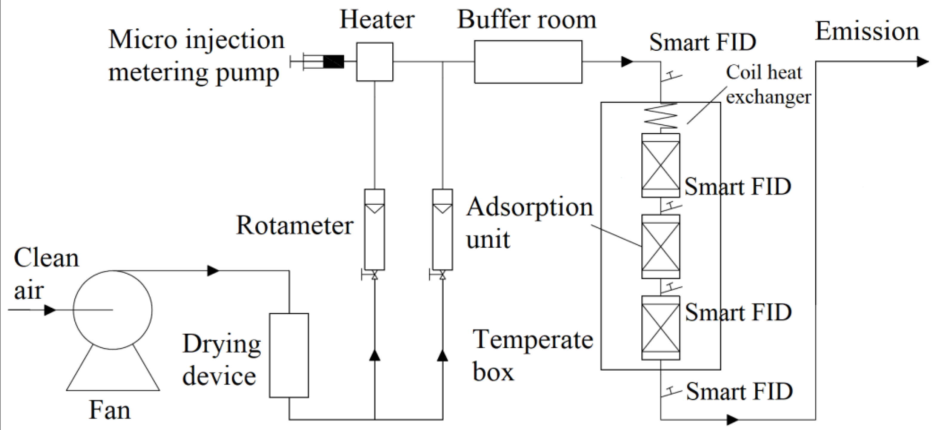
In order to explore the impact of various inlet concentrations of toluene gas on the mass transfer process desorption by activated carbon in closed cycle temperature swing adsorption, we designed four different working conditions. The inlet concentrations were 0, 2, 5 and 10 g/m³. We used an FID to monitor the toluene gas concentration at the outlet of each bed. The desorption unit was composed of three layers of desorption columns. 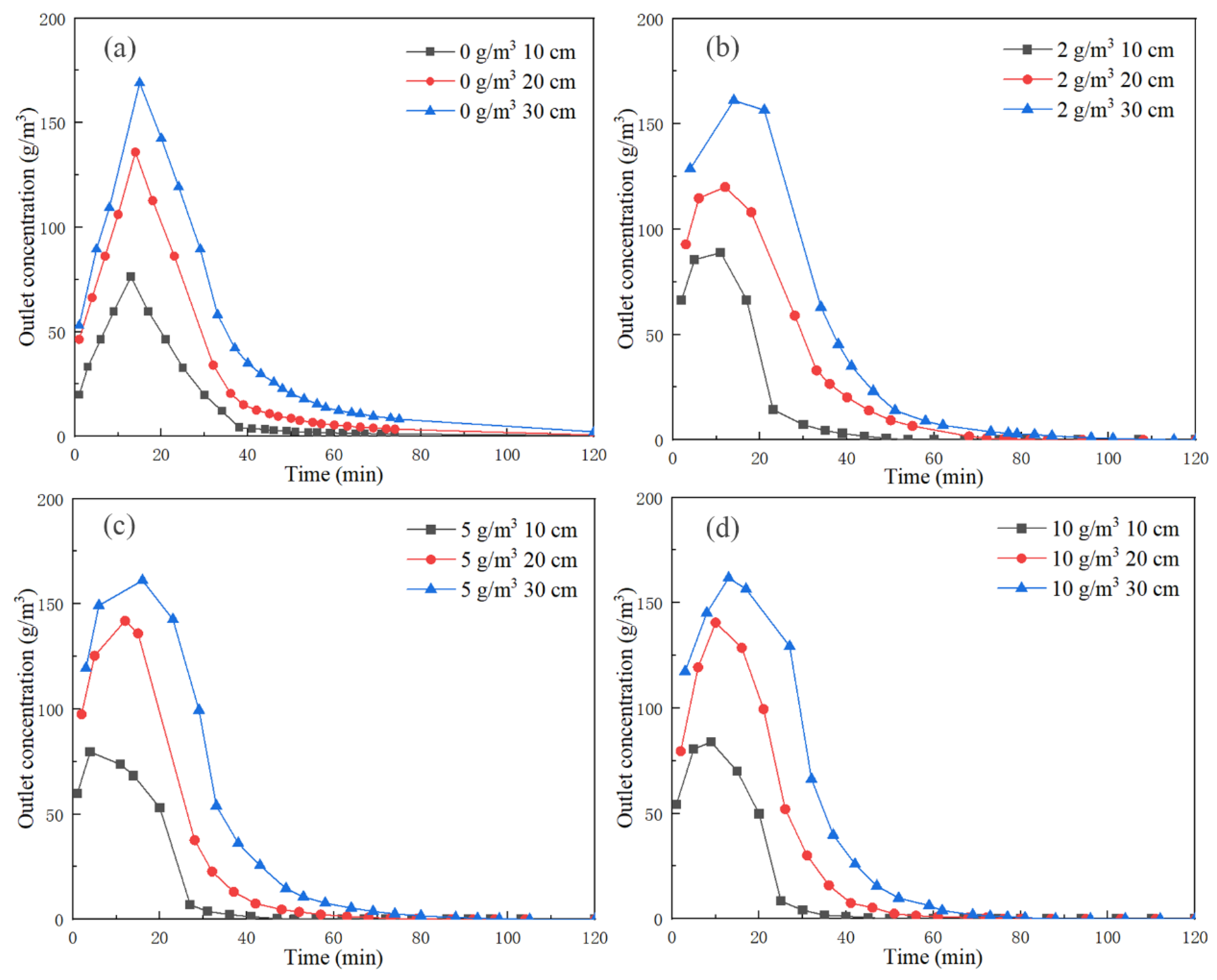Figure 6 shows the outlet concentration curve at the outlet of each bed with various background concentrations (background concentration removed).

In the desorption concentration curves of all background concentrations, the toluene concentration at the outlet section of each bed rapidly rose to a peak, then dropped rapidly and finally stabilized at the background concentration. The toluene outlet concentration measured at 10 cm reached the peak in the shortest time and had the lowest peak concentration. The outlet concentration at 10 cm was the lowest throughout this experiment, and the time to complete desorption and reach equilibrium was the shortest. The time to reach the peak concentration at 30 cm was the longest and the peak concentration was the highest. The outlet concentration at 30 cm was always the highest throughout the experiment, and the time to complete the desorption was the longest. This was due to the fact that during desorption of activated carbon, the rear end activated carbon bed continuously adsorbed a high concentration of toluene desorbed from the front end. After the desorption concentration of the active carbon bed at the front end dropped rapidly, the activated carbon bed at the rear end was no longer affected by the front end desorption, and completely began to desorb.

We compare the outlet concentration curves under different background concentrations in Figure 6. With different background concentrations, the time to reach the peak value did not change significantly and the peak value did not increase or decrease significantly. With the continuous increase in background concentration, the time from complete desorption to the stabilization of equilibrium was shortened. This is because introducing toluene at a specific concentration for desorption increased the outlet concentration of the desorption equilibrium.

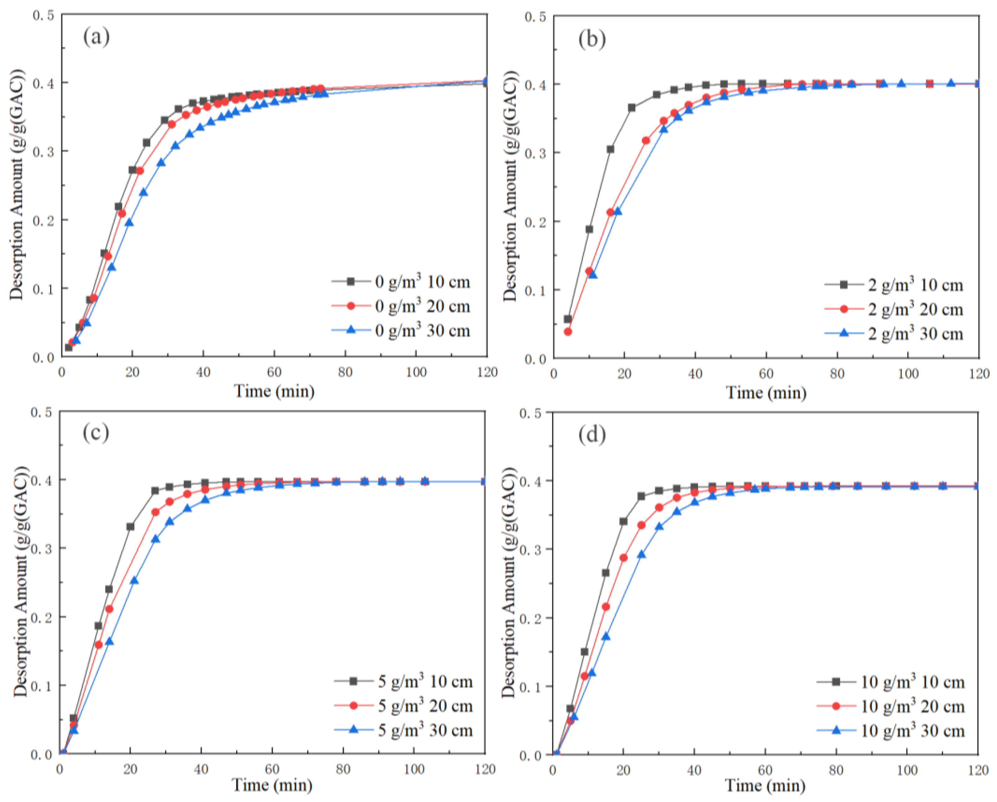
Through integrating the desorption concentration curve in Figure 6, the toluene desorption amount at the outlet of unit activated carbon in each bed under different background concentrations was obtained, and the results are shown in Figure 7. The toluene desorption amount per unit activated carbon of each bed started from zero, rose rapidly in a short time and then tended to be flat and stable. The toluene desorption amount per unit activated carbon at 10 cm was the highest, and the time to reach the inflection point and stabilize was the fastest. The toluene desorption amount per unit activated carbon at 30 cm was the lowest, and the time to reach the inflection point and stabilize was the slowest. Finally, the toluene desorption amount per unit activated carbon in each layer was equal.

Table 4. Data of toluene desorption per unit activated carbon at 120 min for each bed under different working conditions.

Background Concentration (g/m3)	Toluene Desorption per Unit Activated Carbon at 120 min (g/g)
	10 cm	20 cm	30 cm
0	0.398	0.403	0.403
2	0.400	0.400	0.401
5	0.397	0.397	0.397
10	0.392	0.392	0.391

shows a summary of the results of toluene desorption per unit activated carbon at 120 min for each bed under different working conditions.

According to the analysis in Table 4 and Figure 8, under the same desorption temperature and the cross-section wind speed, with the increase background concentration, the time taken from the rapid rise to the inflection point was shorter, and the toluene desorption amount of unit activated carbon outlet gas in each bed layer was lower, but the change was very small.

3.4. Analysis of Average Rate and Instantaneous Rate of Closed Cycle Temperature Swing Desorption

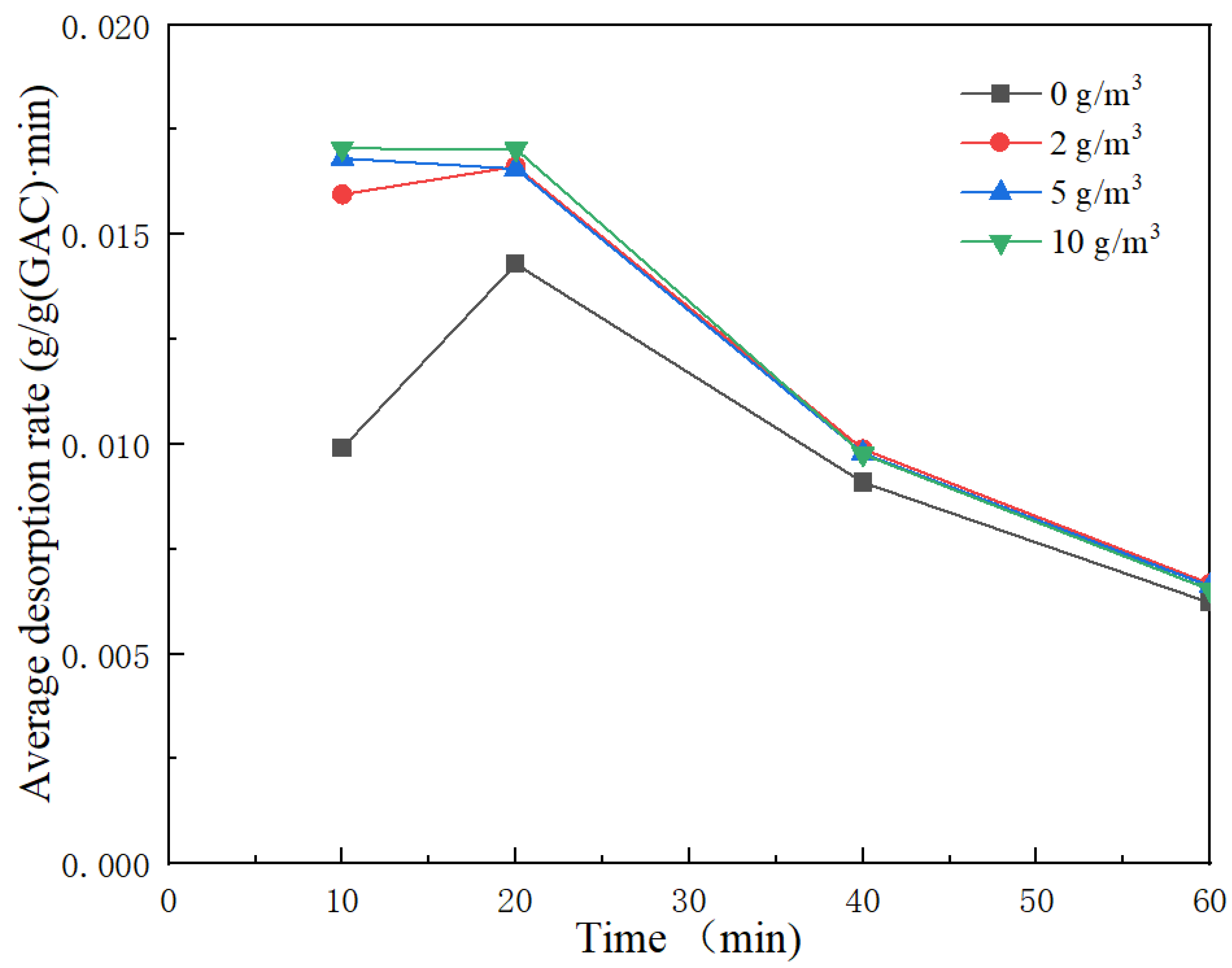
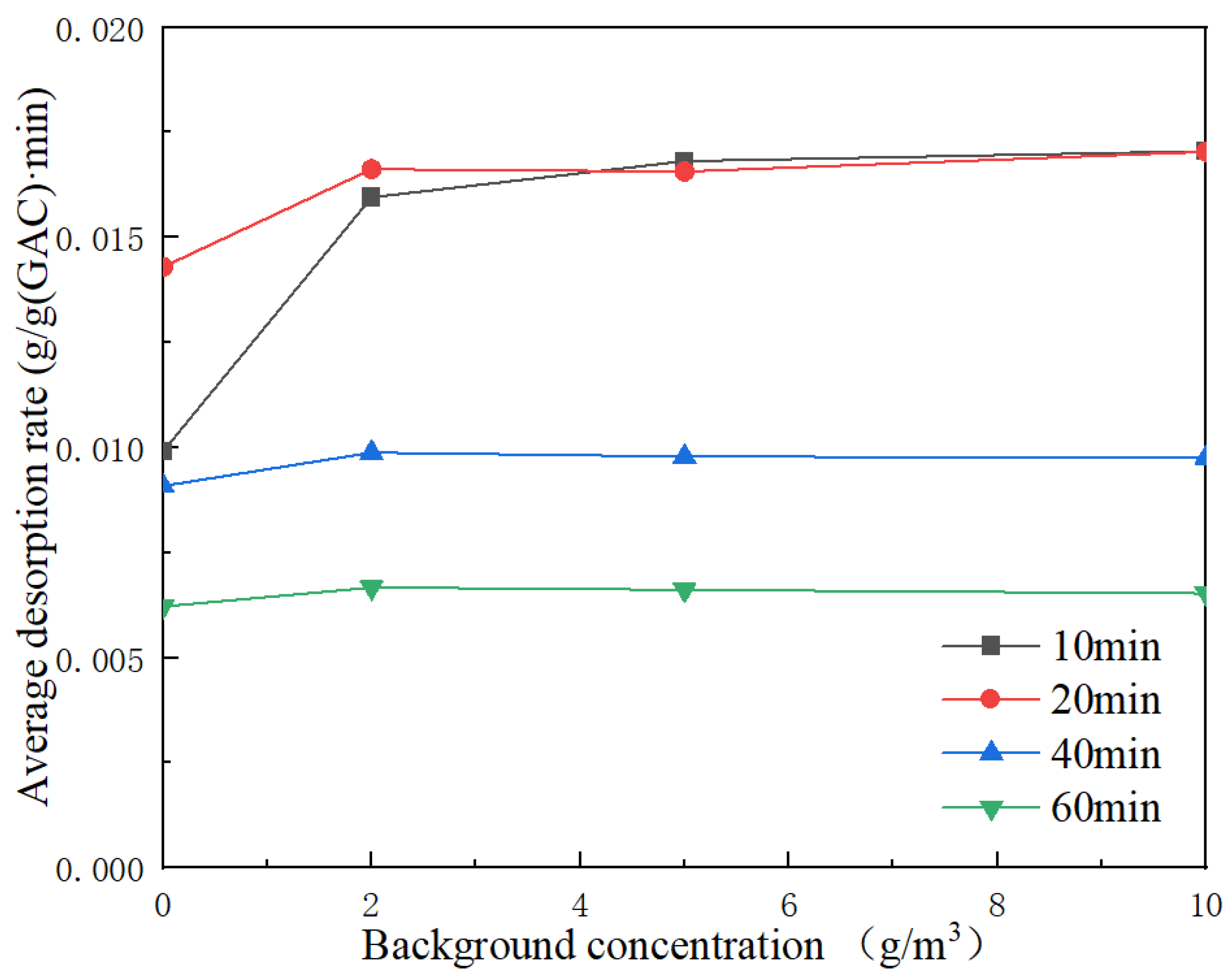
The average desorption rate of unit activated carbon at 10 cm in 10 min is $\stackrel{-}{V_{10}}$ (g/ (g • min)), at 10 cm in 20 min is $\stackrel{-}{V_{20}}$ (g/ (g•min)), at 10 cm in 40 min is $\stackrel{-}{V_{40}}$ (g/ (g•min)) and at 10 cm in 60 min is $\stackrel{-}{V_{60}}$ (g/ (g•min)). Figure 8 shows the average toluene desorption rate of the outlet gas at 10 cm at different times. Figure 9 shows the average toluene desorption rate of outlet gas at 10 cm with different background concentrations.

Under the same working conditions, the $\stackrel{-}{V_{10}}$ at background concentrations of 0, 2, 5 and 10 g/m³ were 0.0099, 0.0160, 0.0168 and 0.0170 g/ (g•min), respectively. The $\stackrel{-}{V_{20}}$ at background concentrations of 0, 2, 5 and 10 g/m³ were 0.0143, 0.0166, 0.0166 and 0.0170 g/ (g•min), respectively. It can be concluded that at the same desorption temperature and the cross-section wind speed, $\stackrel{-}{V_{10}}$ and $\stackrel{-}{V_{20}}$ increase with the increase in background concentration. The 40 min average desorption rates, $\stackrel{-}{V_{40}}$, at background concentrations of 0, 2, 5 and 10 g/m³ were 0.0091, 0.0099, 0.0098 and 0.0098 g/ (g•min), respectively. The 60 min average desorption rates, $\stackrel{-}{V_{60}}$, at background concentrations of 0, 2, 5 and 10 g/m³ were 0.0062, 0.0067, 0.0066 and 0.0065 g/ (g•min), respectively. When the background concentrations were 0–2 g/m³, $\stackrel{-}{V_{40}}$ and $\stackrel{-}{V_{60}}$ also increased as the background concentration increased. $\stackrel{-}{V_{40}}$ and $\stackrel{-}{V_{60}}$ also decreased with the increase in background concentration and tended to be stable when the background concentrations were 2–10 g/m³.

When the background concentrations were 0 and 2 g/m³, the average desorption rate at 10 cm first increased and then decreased, and the average desorption rate at 20 min was the highest. However, when the background concentrations were 5 and 10 g/m³, the average desorption rate at 10 cm declined, and the average desorption rate at 10 min is the highest. Combined with the analysis of the adsorption isotherm in Section 3.1, the adsorption isotherm barely changed when the concentration was between 2 and 10 g/m³. Therefore, when the background concentrations were between 2 and 10 g/m³, the average desorption rate in each period was almost the same.

The average desorption rate at 10 cm under different background concentrations showed a trend of first rising and then declining, and the maximum average desorption rate was $\stackrel{-}{V_{20}}$. $\stackrel{-}{V_{10}}$ reflects the average desorption rate of the initial driving force at the beginning of desorption. $\stackrel{-}{V_{20}}$ reflects the average desorption rate when the initial driving force of desorption is large. $\stackrel{-}{V_{40}}$ reflects the average desorption rate of the driving force in the initial stage of desorption when the concentration of each bed gradually starts to decline gently.

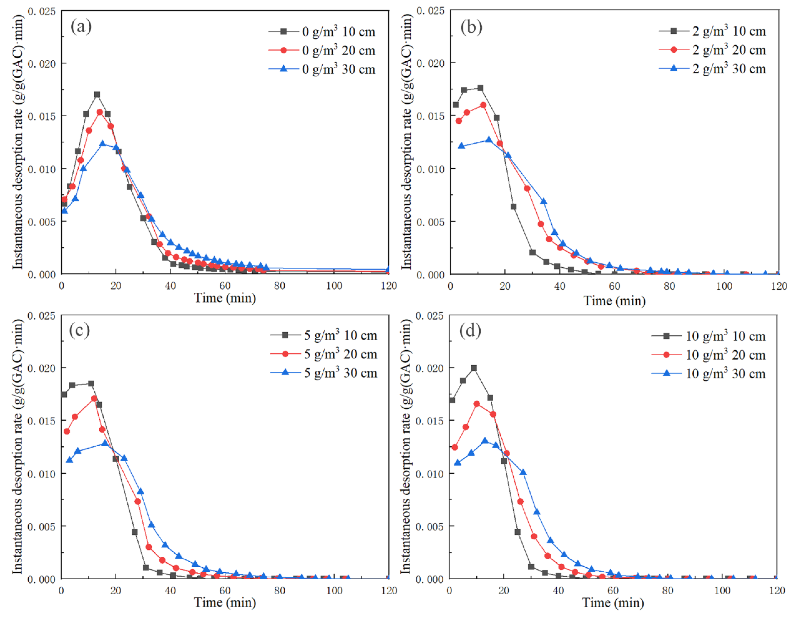
Through the differential of Figure 7, the instantaneous desorption rate of unit activated carbon outlet gas in each bed under different background concentrations was obtained, and the results are shown in Figure 10. At the beginning of the experiment, the instantaneous desorption rate of the unit activated carbon outlet gas in each bed was not zero, and it rapidly rose to the maximum $\stackrel{-}{V_{max}}$ g/(g•min) in a short time, then rapidly dropped to a certain value and slowly became zero. The instantaneous desorption rate of unit activated carbon at 10 cm took the shortest time to reach $\stackrel{-}{V_{max}}$, and it was the highest from the beginning of the experiment to reaching $\stackrel{-}{V_{max}}$, and then dropped rapidly to the minimum until zero. The instantaneous desorption rate of unit activated carbon at 30 cm took the longest time to reach $\stackrel{-}{V_{max}}$, and it was the smallest from the beginning of the experiment to reaching $\stackrel{-}{V_{max}}$.

Table 5. $\stackrel{-}{V_{max}}$ data of each bed under different background concentrations.

Background Concentration (g/m3)	Vmax (g/(g•min))
	10 cm	20 cm	30 cm
0	0.0170	0.0154	0.0123
2	0.0176	0.0160	0.0126
5	0.0185	0.0165	0.0128
10	0.0200	0.0166	0.0131

shows $\stackrel{-}{V_{max}}$ of each bed under different working conditions. At the same desorption temperature and the cross-section wind speed, the higher the background concentration, the larger the desorption $\stackrel{-}{V_{max}}$ at each bed outlet and the faster the time to reach $\stackrel{-}{V_{max}}$. However, when the background concentration was too high, the desorption rate of activated carbon was reduced and the emission of toluene was too large.

3.5. Dynamic Simulation Analysis of Closed Cycle Temperature Swing Desorption

To investigate the effect of closed-cycle temperature swing desorption with different background concentrations on the migration of the adsorbate in the activated carbon layer, the desorption kinetics of toluene between activated carbon beds during desorption were studied by studying the desorption rate.

There are three typical types of kinetic factors, namely the quasi-first-order kinetic equation, the quasi-second-order kinetic equation and the Bangham adsorption rate equation. The differential form of the quasi-first-order kinetic equation is shown in Equation (2) [21,22].

$$\frac{d_{qt}}{d_t}=k_a\left(q_e-q_t\right)$$

(2)

Through the integral of Equation (2), we obtain Equation (3):

$$q_t=q_e {- q}_e{e}^{-k_{a}t}$$

(3)

The differential form of the quasi-second-order kinetic equation is shown in Equation (4) [23].

$$\frac{d_{qt}}{d_t}=k_b{\left(q_e-q_t\right)}^2$$

(4)

Through the integral of Equation (4), we obtain Equation (5):

$$q_t=\frac{k_b{q_e}^{2}t}{1+k_b{q}_{e}t}$$

(5)

The differential form of the Bangham desorption rate equation is shown in Equation (6) [21,22].

$$\frac{d_q}{d_t}=k_c\frac{\left(q_e-q_t\right)}{t^n}$$

(6)

Through the integral of Equation (6), we obtain Equation (7):

$$q_t=q_e {- q}_e{e}^{-k_a{t}^n}$$

(7)

where q_t represents the desorption amount (g/g) at time t, q_e represents the desorption amount at equilibrium (g/g), k_a represents the quasi-first-order desorption rate constant (min⁻¹), k_b represents the quasi-second-order desorption rate constant (min⁻¹), k_c represents the Bangham desorption rate constant (min⁻ⁿ) and n represents the Bangham constant.

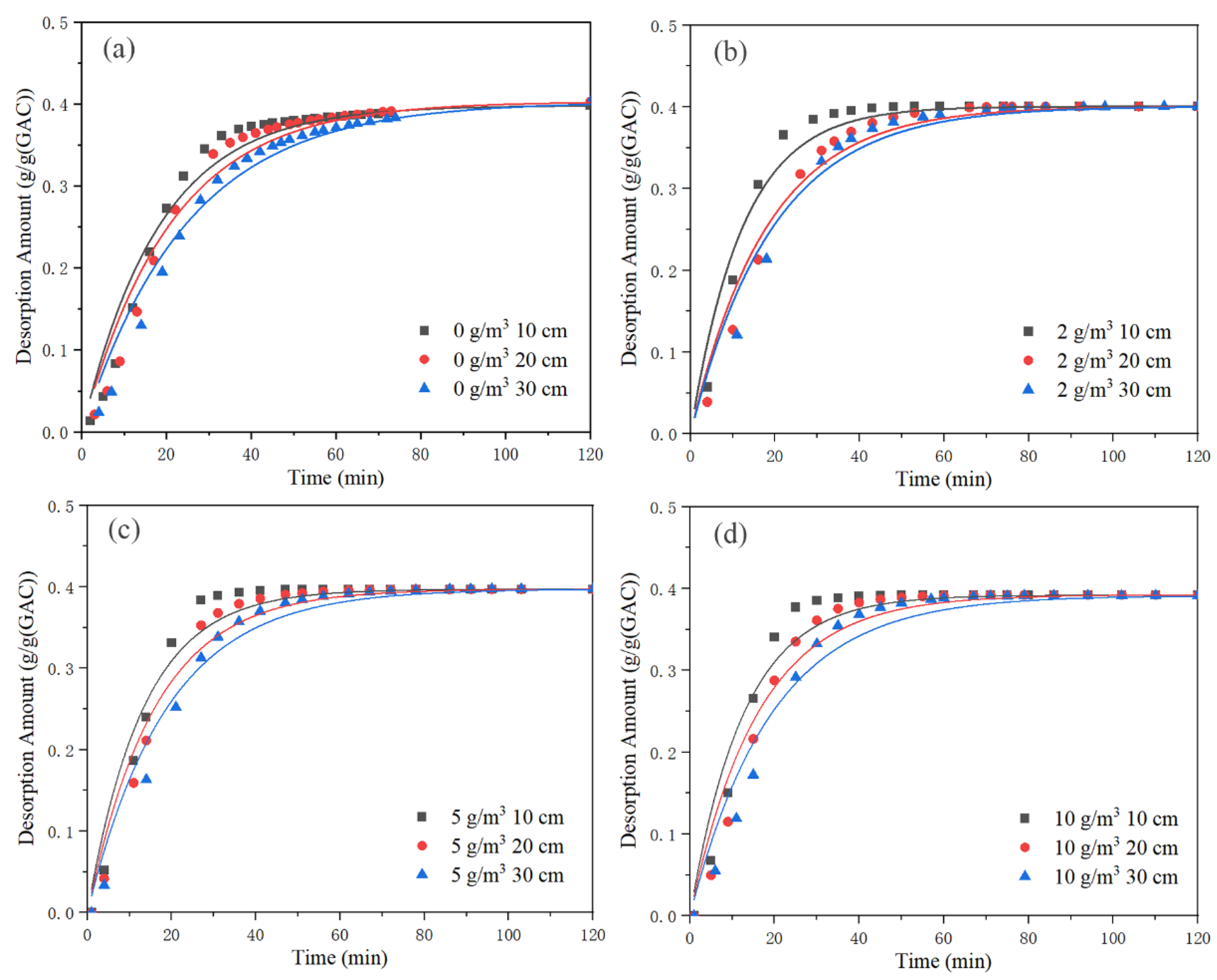
Figure 11 shows the fitting of quasi-first-order kinetic equation for each bed with different background concentrations. The fitting parameters for the quasi-first-order kinetic equation are displayed in

Table 6. The fitting parameters of the quasi-first-order kinetic equation.

Background Concentration (g/m3)	10 cm		20 cm		30 cm
	ka	R2	ka	R2	ka	R2
0	0.0548	0.9626	0.0477	0.9638	0.0404	0.9697
2	0.0808	0.9719	0.0555	0.9786	0.053	0.9749
5	0.0783	0.9677	0.0628	0.974	0.0512	0.9774
10	0.0753	0.9591	0.0623	0.9651	0.0518	0.9641

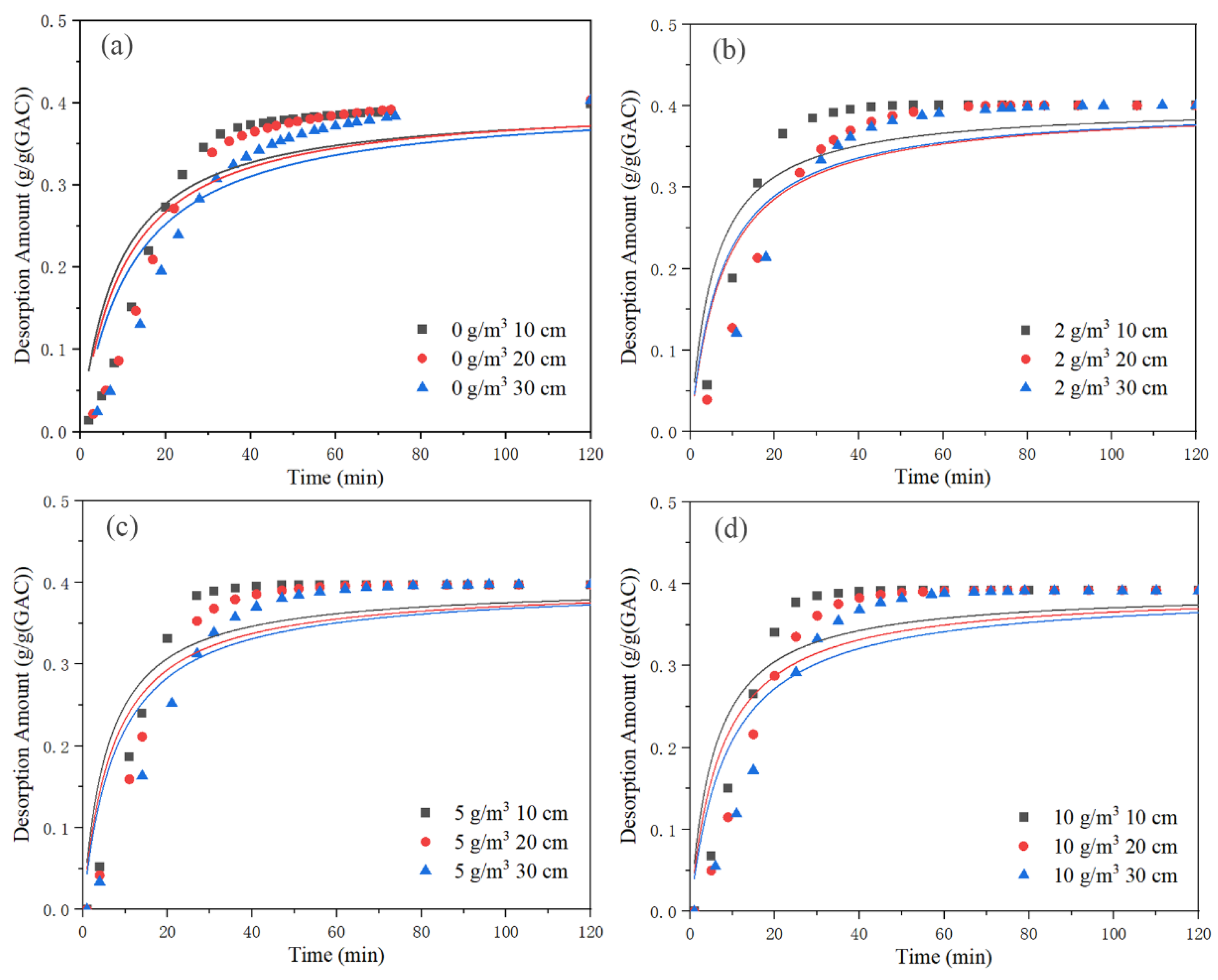
. Figure 12 depicts the fitting of quasi-second-order kinetic equation. The fitting parameters for the quasi-second-order kinetic equation are displayed in

Table 7. The fitting parameters of the quasi-second-order kinetic equation.

Background Concentration (g/m3)	10 cm		20 cm		30 cm
	kb	R2	kb	R2	kb	R2
0	0.2871	0.8162	0.2432	0.8109	0.208	0.8234
2	0.4462	0.8507	0.3599	0.8572	0.324	0.8411
5	0.4445	0.839	0.3556	0.8482	0.3136	0.8605
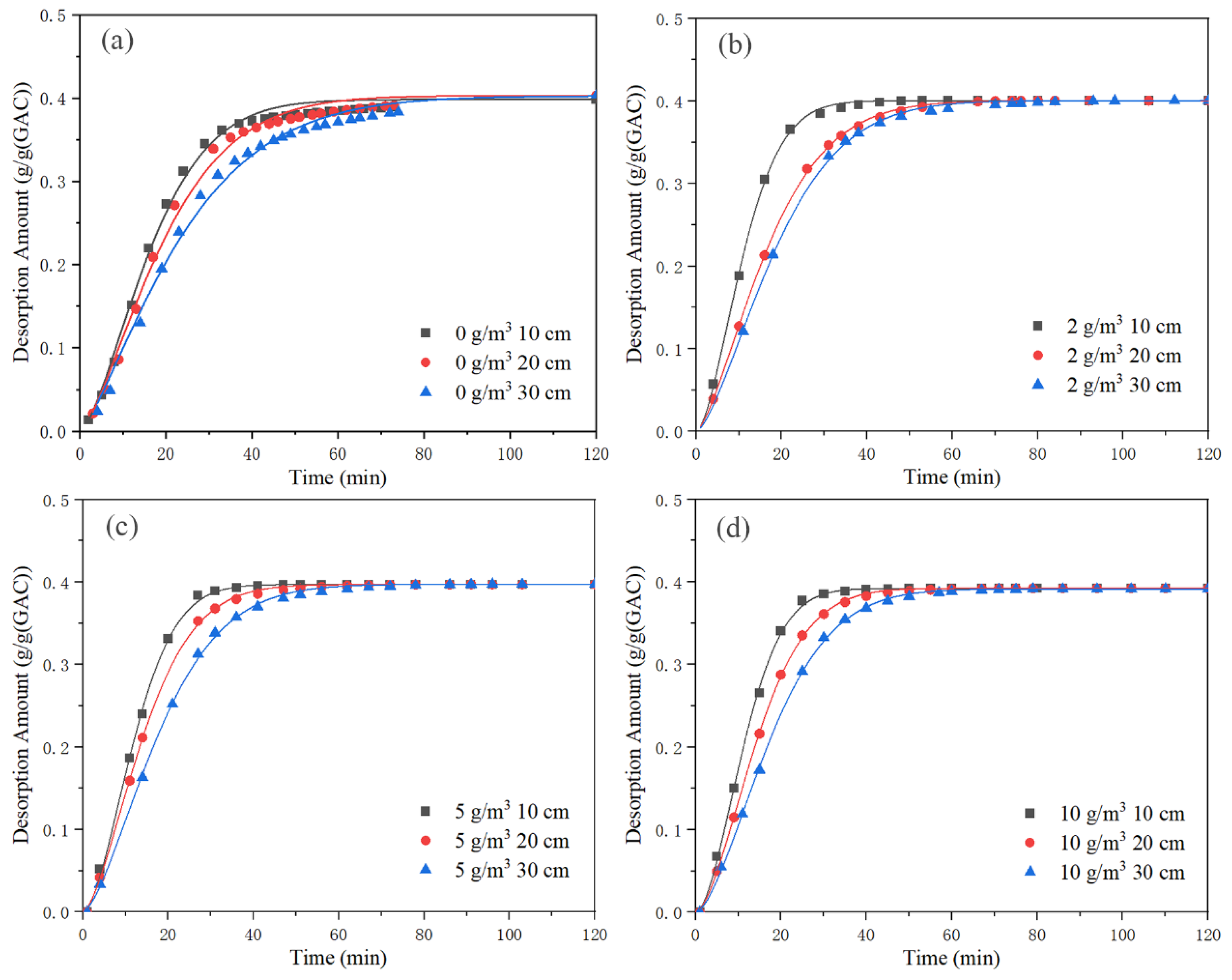
10	0.4267	0.8205	0.3483	0.8285	0.291	0.8212

. The Bangham desorption rate equation’s fit is depicted in Figure 13. The fitting parameters for the Bangham desorption rate equation are displayed in

Table 8. The fitting parameters of the Bangham desorption rate equation.

Background Concentration (g/m3)	10 cm			20 cm			30 cm
	kc	n	R2	kc	n	R2	kc	n	R2
0	0.0131	1.499	0.9931	0.013	1.404	0.9924	0.0102	1.3024	0.991
2	0.0152	1.6326	0.9994	0.0139	1.4421	0.9997	0.0104	1.4845	0.9992
5	0.0129	1.7001	0.9992	0.0125	1.555	0.9996	0.0099	1.5189	0.9993
10	0.0102	1.7578	0.9994	0.0093	1.6489	0.9998	0.0078	1.6049	0.9997

. The value of q_e was taken from the data in Table 4. According to Figure 11 and Table 6, the R² value of the quasi-first-order kinetic equation was greater than 0.9591, and the fit was good. According to Figure 12 and Table 7, the R² value of the quasi-second-order kinetic equation was less than 0.90, and the fit was poor. According to Figure 13 and Table 8, the R² value of the Bangham desorption rate equation was greater than 0.99, and the fit was the best out of the three equations. The three kinetic models’ desorption rate constants rose initially, then fell as background concentration rose. A background concentration of 2 g/m³ resulted in the highest desorption rate constant. However, when the saturated activated carbon was desorbed by clean gas, the desorption rate constant was low. The Bangham constant increased with the increase in background concentration. The desorption rate constants of the three kinetic models decreased with the increase in activated carbon bed length. This is similar to the analysis of average desorption rate and instantaneous desorption rate. It shows that under the conditions of closed cycle adsorption, the concentration polarization layer of activated carbon was broken when a certain concentration of toluene was purged. While the external diffusion mass transfer effect increased, the internal mass transfer resistance decreased.

4. Conclusions

Toluene was chosen as this research’s VOC representative target pollutant. By using the desorption amount, average desorption rate and instantaneous desorption rate as evaluation factors, process conditions such as the length of activated carbon layer and background concentration of desorption gas were simulated. The following conclusions were drawn from the experimental results:

• When the activated carbon desorbs, the rear end activated carbon bed continuously absorbs the high concentration of toluene desorbed from the front end. After the desorption concentration of the active carbon bed at the front end dropped rapidly, the activated carbon bed at the rear end was no longer affected by the front end desorption, and began to completely desorb. When the background concentration was 0 g/m³, the toluene desorption per unit activated carbon at 120 min at 20 and 30 cm were the largest, both at 0.403 g/g.
• The average desorption rate under different background concentrations showed a trend of first rising and then declining, and the maximum average desorption rate was $\stackrel{-}{V_{20}}$. $\stackrel{-}{V_{20}}$ at background concentrations of 0, 2, 5 and 10 g/m³ were 0.0143, 0.0166, 0.0166 and 0.0170 g/ (g•min), respectively. $\stackrel{-}{V_{10}}$ reflects the average desorption rate of the initial driving force at the beginning of desorption. $\stackrel{-}{V_{20}}$ reflects the average desorption rate when the initial driving force of desorption is large. When the background concentration was 10 g/m³, $\stackrel{-}{V_{10}}$ and $\stackrel{-}{V_{20}}$ were the largest, both 0.0170 g/ (g•min). $\stackrel{-}{V_{40}}$ reflects the average desorption rate of the driving force in the initial stage of desorption when the concentration of each bed gradually starts to decline. When the background concentration was 2 g/m³, $\stackrel{-}{V_{40}}$ and $\stackrel{-}{V_{60}}$ were the largest, at 0.0099 and 0.0067 g/ (g•min), respectively.
• At the same desorption temperature and cross-section wind speed, the higher the background concentration, the larger the desorption $\stackrel{-}{V_{max}}$ at each bed outlet and the faster the time to reach $\stackrel{-}{V_{max}}$. When the desorption temperature was 150 ℃, the cross-section wind speed was 0.2 m/s, the background concentrations were 0, 2, 5 and 10 g/m³ and the unit activated carbon $\stackrel{-}{V_{max}}$ at 10 cm was 0.0170, 0.0206, 0.0185 and 0.0200 g/ (g•min), respectively.
• Among the three kinetic models, the fitting effect of Bangham desorption rate equation was the best, as the R² value was greater than 0.99. The desorption rate constant was the highest when the background concentration was 2 g/m³ and the activated carbon layer length was 10 cm, with a value of 0.0152 min⁻¹.

This study simplified the subjects and experimental conditions. It is anticipated that it will offer a theoretical framework for a more extensive, precise and efficient application of activated carbon closed-cycle temperature swing desorption of VOCs.

References

1. Dumanoglu, Y.; Kara, M.; Altiok, H.; Odabasi, M.; Elbir, T.; Bayram, A. Spatial and seasonal variation and source apportionment of volatile organic compounds (VOCs) in a heavily industrialized region. Atmos. Environ. 2014, 98, 168–178. [Google Scholar] [CrossRef]
2. Dunmore, R.E.; Hopkins, J.R.; Lidster, R.T.; Mead, M.I.; Bandy, B.J.; Forster, G.; Oram, D.E.; Sturges, W.T.; Phang, S.M.; Samah, A.A.; et al. Development of a combined heart-cut and comprehensive two-dimensional gas chromatography system to extend the carbon range of volatile organic compounds analysis in a single instrument. Separations 2016, 3, 21. [Google Scholar] [CrossRef] [Green Version]
3. Cai, W.; Wang, M.; Yang, G.Q.; Zhang, Z.; Wang, Y.; Li, J. Study of the dissolution and diffusion of propane, propylene and nitrogen in polydimethylsiloxane membranes with molecular dynamics simulation and Monte Carlo simulation. Separations 2022, 9, 116. [Google Scholar] [CrossRef]
4. Zhang, X.; Gao, B.; Creamer, A.E.; Cao, C.; Li, Y. Adsorption of VOCs onto engineered carbon materials: A review. J. Hazard. Mater. 2017, 338, 102–123. [Google Scholar] [CrossRef] [PubMed]
5. Parmar, G.R.; Rao, N.N. Emerging control technologies for vlatile organic compounds. Crit. Rev. Environ. Sci. Technol. 2008, 39, 41–78. [Google Scholar] [CrossRef]
6. Mohamed, E.F.; Awad, G.; Andriantsiferana, C.; EI-Diwany, A.I. Biofiltration technology for the removal of toluene from polluted air using Streptomyces griseus. Environ. Technol. 2015, 131, 1197–1207. [Google Scholar]
7. Choi, B.S.; Yi, J. Simulation and optimization on the regenerative thermal oxidation of volatile organic compounds. Chem. Eng. J. 2000, 76, 103–114. [Google Scholar] [CrossRef]
8. Choudhary, T.V.; Banerjee, S.; Choudhary, V.R. Catalysts for combustion of methane and lower alkanes. Appl. Catal. A Gen. 2002, 234, 1–23. [Google Scholar] [CrossRef]
9. Ma, X. Reactive adsorption of gaseous anisole by MCM–41-supported sulfuric acid. Catalysts 2022, 12, 942. [Google Scholar]
10. Liu, L.; Tian, S.; Ning, P. Phase behavior of tweens/toluene/water microemulsion systems for the solubilization absorption of toluene. J. Solut. Chem. 2010, 39, 457–472. [Google Scholar]
11. Xu, H.; Xu, X.; Chen, L.; Guo, J.; Wang, J. A novel cryogenic condensation system combined with gas turbine with low carbon emission for volatile compounds recovery. Energy 2022, 248, 123604. [Google Scholar] [CrossRef]
12. Wang, S.; Zhang, L.; Long, C.; Li, A. Enhanced adsorption and desorption of VOCs vapor on novel micro-mesoporous polymeric adsorbents. Chem. Eng. Sci. 2014, 428, 185–190. [Google Scholar] [CrossRef] [PubMed]
13. Sahin, S. Fabrication and characterization of 3,4-diaminobenzophenone-functionalized magnetic nanoadsorbent with enhanced VOC adsorption and desorption capacity. Environ. Sci. Pollut. Res. 2021, 28, 5231–5253. [Google Scholar] [CrossRef]
14. Yang, X.; Ren, X.; Yan, X.; Wu, Z.; Yang, G. A review on VOCS adsorption by activated carbon. Mater. Rep. 2021, 35, 17111–17124. [Google Scholar]
15. Sheintuch, M.; Matatov-Meytal, Y. Comparison of catalytic processes with other regeneration methods of activated carbon. Catal. Today 1999, 53, 73–80. [Google Scholar] [CrossRef]
16. Chen, J.; Qin, Y.; Chen, Z.; Yang, Z.; Yang, W.; Wang, Y. Gas circulating fluidized beds photocatalytic regeneration of I-TiO2 modified activated carbons saturated with toluene. Chem. Eng. J. 2016, 293, 281–290. [Google Scholar] [CrossRef]
17. Veleva, V.; Bodkin, G. Corporate-Entrepreneur collaborations to advance a circular economy. J. Clean. Prod. 2018, 188, 20–37. [Google Scholar] [CrossRef]
18. Zhen, X.; Qiu, W.; Dou, K.; Huang, H. Desorption of toluene on activated carbon by thermal nitrogen. Energy Environ. Prot. 2020, 34, 15–19. [Google Scholar]
19. Lv, X.; Qi, Q.; Bai, G.; Zhu, J.; Zhang, W.; Liang, P. Study on adsorption and desorption performance of spherical activated carbon and spherical polymer resin for different volatile organic compounds. J. Shandong Univ. Sci. Technol. 2019, 38, 58–64. [Google Scholar]
20. Muttakin, M.; Mitra, S.; Thu, K.; Ito, K.; Saha, B.B. Theoretical framework to evaluate minimum desorption temperature for IUPAC classified adsorption isotherms. Int. J. Heat Mass Transf. 2018, 122, 795–805. [Google Scholar] [CrossRef]
21. Hashisho, Z.; Emamipour, H.; Cevallos, D.; Rood, M.J.; Hay, K.J.; Kim, B.J. Rapid response concentration-controlled desorption of activated carbon to dampen concentration Fluctuations. Environ. Sci. Technol. 2007, 41, 1753–1758. [Google Scholar] [CrossRef] [PubMed]
22. Raganati, F.; Alfe, M.; Gargiulo, V.; Chirone, R.; Ammendola, P. Kinetic study and breakthrough analysis of the hybrid physical/chemical CO2 adsorption/desorption behavior of a magnetite-based sorbent. Chem. Eng. J. 2019, 372, 526–535. [Google Scholar] [CrossRef]
23. Mahanta, D.; Madras, G.; Radhakrishnan, S.; Patil, S. Adsorption and desorption kinetics of anionic dyes on doped polyaniline. J. Phys. Chem. B 2009, 113, 2293–2299. [Google Scholar] [CrossRef] [PubMed]
Figure 1. Dynamic adsorption experimental device.
Separations 10 00213 g001
Figure 2. Desorption experimental device.
Separations 10 00213 g002
Figure 3. Adsorption isothermal curve of activated carbon for toluene.
Separations 10 00213 g003
Figure 4. Langmuir and Freundlich fitting curve of the adsorption isothermal curves.
Separations 10 00213 g004
Figure 5. Working capacity curves of activated carbon with different toluene gas concentrations under different closed cycle condensation temperatures.
Separations 10 00213 g005
Figure 6. Outlet concentration curves of toluene gas at each bed outlet with different background concentrations. (background concentration has been removed). (a) 0 g/m3, (b) 2 g/m3, (c) 5 g/m3, (d) 10 g/m3.
Separations 10 00213 g006
Figure 7. Desorption amount of toluene in the outlet gas of each bed with different background concentrations. (a) 0 g/m3, (b) 2 g/m3, (c) 5 g/m3 and (d) 10 g/m3.
Separations 10 00213 g007
Figure 8. Average desorption rate of toluene at 10 cm outlet gas at different times.
Separations 10 00213 g008
Figure 9. Average desorption rate of toluene in the outlet gas at 10 cm with different background concentrations.
Separations 10 00213 g009
Figure 10. Instantaneous toluene desorption rate of gas at the outlet of each bed with different background concentrations. (a) 0 g/m3, (b) 2 g/m3, (c) 5 g/m3 and (d) 10 g/m3.
Separations 10 00213 g010
Figure 11. The quasi-first-order kinetic equation fit for each bed with different background concentrations. (a) 0 g/m3, (b) 2 g/m3, (c) 5 g/m3 and (d) 10 g/m3.
Separations 10 00213 g011
Figure 12. The quasi-second-order kinetic equation fit for each bed with different background concentrations. (a) 0 g/m3, (b) 2 g/m3, (c) 5 g/m3 and (d) 10 g/m3.
Separations 10 00213 g012
Figure 13. The Bangham desorption rate equation fit for each bed with different background concentrations. (a) 0 g/m3, (b) 2 g/m3, (c) 5 g/m3 and (d) 10 g/m3.
Separations 10 00213 g013