Simulation of Water Vapor and Near Infrared Radiation to Predict Vapor Pressure Deficit in a Greenhouse Using CFD

Abstract

Vapor pressure deficit (VPD) can be used as an indicator to schedule greenhouse irrigation. VPD can be estimated as a function of relative humidity (RH) and temperature (T). The objective of this work was to analyze spatial variation in VPD as an indicator of water stress influenced by concentration of water vapor and intensity of near infrared (NIR). The study was carried out in an empty three-span sawtooth greenhouse with natural ventilation under the local climate in Montecillo, Mexico; these findings established a base value to analyze greenhouse field conditions prior to the influence from a crop. The experimental phase consisted of recording data (3 February 2019–24 February 2019) on temperature, humidity, solar radiation, and wind speed, which were used for developing a model in computational fluid dynamics (CFD). Then, this model was used to estimate VPD, considering changes in mass fraction of water vapor and the intensity of NIR. Scenarios with 50, 70, and 90% external RH were evaluated. It was found that without a crop, temperature was not affected by the variation in the mass fraction of water vapor and the intensity of NIR in the simulated scenarios, each of which generated a thermal gradient within the range of 4 °C. When considering the scenario of 90% external RH, we found the best VPD range along the greenhouse (2–3 kPa) that would be a favorable field condition for crops. Differences between VPD with and without a crop can be used to estimate the water quantity needs for crop growth based on the climate variables examined in this study, where higher VPD values require more water for irrigation.

1. Introduction

In greenhouses, the ventilation system favors the distribution of temperature inside. With natural ventilation, air exchange sometimes becomes insufficient due to outside wind speeds equal to or less than 1 m s⁻¹, causing an increase in temperature and reducing the concentration of CO₂ and relative humidity [% (RH)] [1,2,3]. In 2017, Cemek et al. [4] concluded that ventilation efficiency should be further analyzed with the aim of establishing the best environmental conditions favoring plant growth parameters. Wind speed and direction are factors impacting the environmental comfort of the internal climate of a greenhouse, specifically in terms of the exchange of heat and mass between the inside and outside [5,6,7]. The ventilation system of a greenhouse may eliminate excess heat and maintain acceptable CO₂ and water vapor levels for crops [8,9]. Strategies of natural ventilation are diversified according to the season of the year; for instance, during winter, natural ventilation allows the elimination of excess humidity, while in summer it sometimes provides insufficient cooling, requiring the use of auxiliary mechanical ventilation systems [10].

One of the parameters for greenhouse climate management that integrates temperature and relative humidity in a single value, used as an indicator of water vapor environment, is the vapor pressure deficit (VPD). Fernández et al., Prenger and Ling, and Dik and Wubben [11,12,13] mention that VPD is a tool that can be used for climate, water, and disease management within the greenhouse. López and Shtienberg [14,15] point out that a VPD greater than 1.25 kPa in a greenhouse generates a high transpiration rate of plants, so it is important to maintain VPD levels. VPD can be used as an indicator to infer the time to apply irrigation because it measures the amount of water that the surrounding atmosphere can receive. Veluzan [16] mentions that the loss of water by a plant depends on the VPD; when the VPD increases, the plant begins to perspire, and when it reaches 2 kPa, stomatal closure may be observed, reducing plant growth. The planning and management of VPD values in a greenhouse imply a knowledge of the levels of humidity (RH) and radiation (NIR) that prevail during different seasons.

Similarly, the distribution of solar radiation in a greenhouse is important because it is an input and the driving force of the physiological functions of plants. Solar radiation is the main factor for crop growth inside greenhouses, having an indirect impact on air temperature and regulating two physiological phenomena in plants: (i) transpiration and (ii) photosynthesis [17]. The energy consumption of a greenhouse depends on the incoming solar radiation [18], which is influenced by the greenhouse design (orientation and shape of the roof), the thermo-physical and optical properties of the cladding, and the climate [19]. Therefore, the orientation and shape of the roof become the most important physical elements in the distribution of solar radiation [20,21,22].

Solar radiation is a factor used to determine the energy balance of greenhouses. A numerical model makes it possible to estimate transmission of solar radiation, emphasizing the properties of cladding materials [23]. In the 1980s, dynamic models of the greenhouse climate were developed with the aim of calculating effects of solar radiation on the quality and production of crops [24,25]. Solar radiation modeling was initially approached indirectly using analytical models to calculate the surface temperatures that developed due to short- and long-wave radiation [26]. Likewise, the radioactive effect as a heat source was estimated in the energy equation attributed to short-wave and thermal solar radiation emitted by heated surfaces [27].

Water vapor absorbs and emits more infrared radiation in the atmosphere; its concentration increases as global warming increases [28,29], inducing an increase in environmental evaporation because the saturated water vapor margin widens due to the increase in temperature. Water vapor participates as a greenhouse gas, having an impact on atmospheric structure and the precipitation regime [30]. Water vapor is characterized by absorbing at wavelengths centered at 940, 1100, 1380, and 1870 nm, between 80 and 99.5% of solar energy at these lengths. Water vapor absorbs more near-infrared (NIR) radiation than any other component in the atmosphere. Under atmospheric conditions and a clear sky (no clouds), the water vapor absorbs approximately 43 W m⁻² of the annual average of incident solar radiation [31]. Of this absorbed solar radiation, 98% belongs to the near infrared (NIR) zone, that is to say, wavelengths greater than 0.7 µm [32].

In more recent years, computational models have been used to solve radiation transport, the most popular being the discrete ordinate (DO) model used by ANSYS FLUENT [8,33,34,35,36]. The DO model bases its calculations on solving the short-wave and long-wave radioactive transfer equations (RTE) [33,37,38,39,40]. It is useful for calculating surface-to-surface radiation exchanges, but not for transfers within the canopy [41].

Full-scale simulations with 2D and 3D CFD models have been used to study the microclimate distribution in greenhouses through the incorporation of solar radiation models and sensible and latent heat exchange sub-models [42]. Likewise, these models were used to evaluate the environmental effect in the greenhouse caused by its design [43], cladding material [44], time of day, season of the year [45,46], the type of ventilation, and its configuration [47]. However, scarce or no information is available to analyze the effect of the intensity of NIR and the concentration of water vapor on the air temperature of a greenhouse [48,49,50]. VPD is the difference between the amount of water in air as vapor and the amount of moisture the air can retain when it is saturated with water, so it can be considered a useful way to measure the microclimate of a greenhouse; the value of VPD can be estimated through the equation of Rosenberg et al. [51], VPD = 0.61078exp [(17.269 · T)/(T + 237.3)] · [1 + RH/100], where T is the air temperature.

The objective of this work was to develop and evaluate a computational model to estimate VPD values as an indicator of water stress, due to the relationship between water quantity or vapor concentration (RH) and NIR in the greenhouse environment. The idea of simulating an empty greenhouse assumed that the exchange of mass and energy between the exterior and interior of the greenhouse only occurs through natural ventilation, and there is no generation of water vapor inside the greenhouse. Predicting VPD values without cultivation facilitates an easier understanding of the requirements to achieve recommended ranges.

2. Materials and Methods

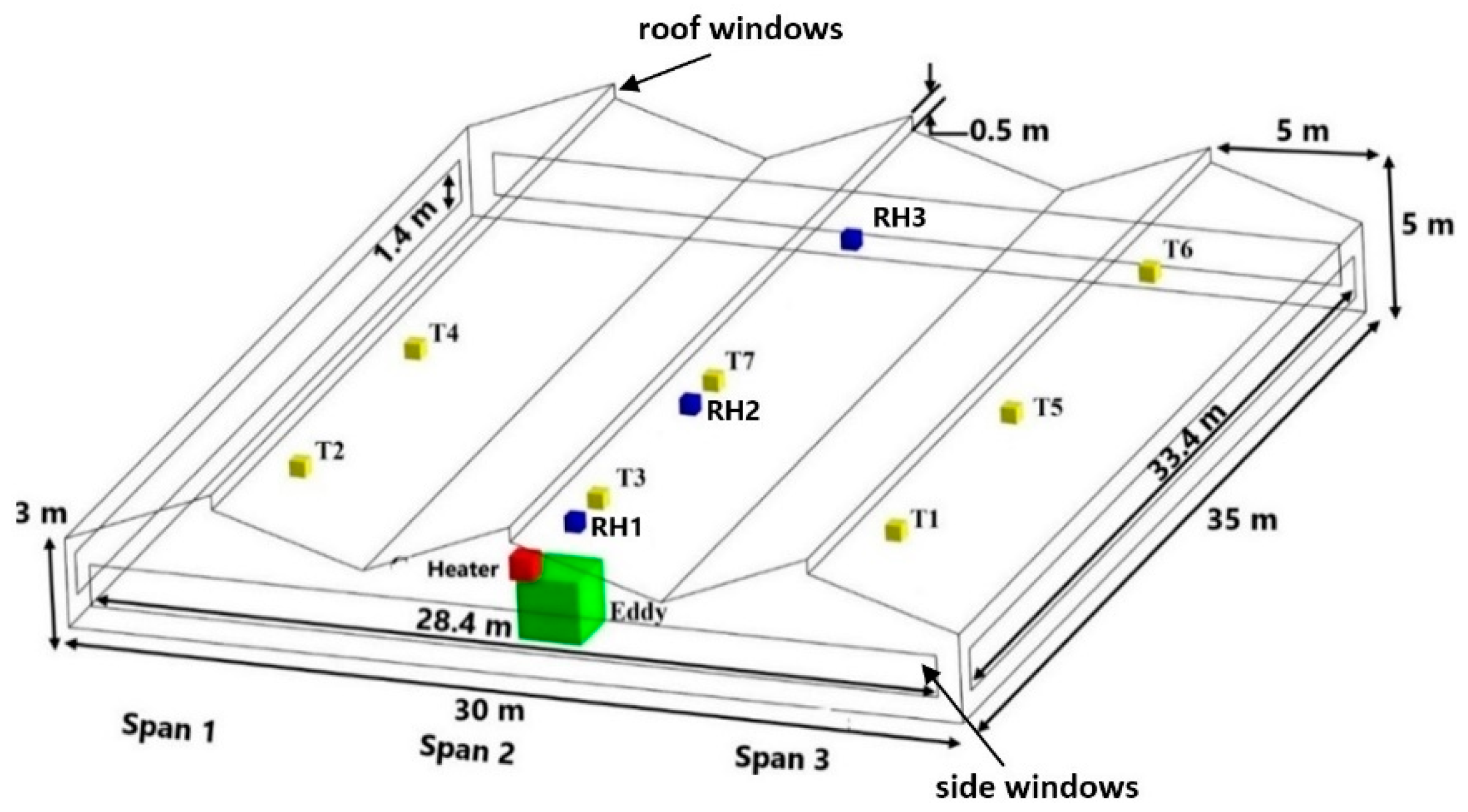
2.1. Description of Experimental Site

The greenhouse used in this study is located at Campus Montecillo, Colegio de Postgraduados in the State of Mexico (19°27′45.5” N, 98°54′12.2” W) with an altitude of 2239 masl, oriented from north to south on a plain where monthly mean temperatures range from 5 to 25 °C. It has an area of 1050 m²; it is a three-span sawtooth type covered with translucent polyethylene on the floor and sides, polycarbonate on the roof, and anti-insect mesh on three side windows and three roof windows. The greenhouse relies on a natural ventilation system with the roof and side windows fully open.

For data acquisition, an eddy covariance system was installed at a distance of 2.4 m, windward, equipped with a sonic anemometer (3D, Campbell Scientific Ltd., Antony, France), an EC150 gas analyzer (Campbell Scientific Inc., Logan, UT, USA), a net radiometer (NR-LITE2 Kipp and Zone BV, Delft, The Netherlands), an LI-200 pyranometer (LI-COR Inc., Lincoln, NE, USA), an LI-190R Quantum sensor (Li-Cor Inc., Lincoln, NE, USA), a temperature and humidity sensor (HMP155A, Campbell Scientific, Logan, UT, USA), and four sensors for recording soil temperature (TCAV thermocouple, Campbell Scientific Inc., Logan, UT, USA). Seven temperature sensors (DS18B20, Maxim Integrated, San Jose, CA, USA) and three humidity sensors (DHT22, Zhengxinyuan Electronics Co., Ltd., Shenzhen, China) were installed in distributed locations in the three spans at a height of 3 m (Figure 1).

Data logging and storage were performed every 5 s for temperature and humidity, 100 ms for the anemometer, and 20 s for the net radiometer. The monitoring period was during the month of February 2019, the month when there commonly is a RH gradient that oscillates between 30–100% inside the greenhouse between the day and night periods, respectively. During data collection, there was no crop, thus the humidity inside the greenhouse came from outside. Information storage was carried out with a data logger system (CR3000 Micrologger, Campbell Scientific, Inc., Logan, UT, USA) for the eddy covariance system, and an Arduino Data Logger Shield for the DS18B20 and DHT22 sensors. Outside the greenhouse there was a meteorological station (Vantage Pro2 Plus, Davis Instruments, Hayward, CA, USA) used to collect data on temperature, humidity, solar radiation, and wind direction and speed—measurements that were used as the initial boundary conditions of the computational model. The stored information was downloaded and processed in Microsoft Excel to determine the input environmental conditions of the computational model.

2.2. Computational Model

The computational model was developed and simulated in ANSYS^® Fluent^®. The geometry was developed in ANSYS^® Workbench using the SpaceClaim tool. The mesh of the model domain was built in Meshing. The properties of the greenhouse materials were incorporated into the model following

Table 1. Properties of cladding materials.

Material	Density (ρ) (kg m−3)	Specific Heat (CP) (J kg−3 °C−1)	Thermal Conductivity (k) (W m−1 °C−1)	Thickness (mm)
Soil	1300	800	1
Wall and mulch (Polyethylene PE)	925.5	1900	0.3	0.18
Roof (Polycarbonate PC)	1200	1200	0.19	6

and

Table 2. Optical properties of materials to thermal radiation.

Materials	Emissivity (Ɛ)	Transmissivity (τ)	Reflectivity (δ)
Polycarbonate	0.935	0.25	0.09
Polyethylene	0.8	0.1	0.03
Soil	0.95		1.92
Air	0.0015		1.009

[8,19,44,52]. Mesh sensitivity analysis of the model was performed to obtain reliable predictions in the same way as in [53]. Mesh was built with structured elements, using an orthogonal quality of 0.98 and distortion of 1.935 × 10^−0.02.

The conditions of the model and of the variables applied to the air flow to solve the transport equations discretized in algebraic equations and calculated by numerical methods are defined in

Table 3. Settings of the computational model.

Condition	Method
Solver	Pressure-based
Analysis Type	Steady
Viscosity Model	Sstandar k-ε (2 equations)
Energy model	Turn on
Radiation model	Discrete ordinate (DO)
Grey longwave	NIR 0.76–1.1 µm
Species	Mass fraction constant
Boundary conditions
Air Temperature	Constant (22 °C)
Air Flow Rate	Constant (3136 kg s−1)
Porous jump	Permeability face, thin porous media and drag coefficient
Heat source	Constant from soil (44.1 °C)

. For the species model, the mass fraction of water vapor was used to calculate the relative humidity distribution.

2.3. Fundamental Equations of Modeled Flow

The general transport equation that can be solved numerically by CFD to explicitly calculate the velocity and temperature field associated with a flow in three dimensions at steady state can be described in the following terms [19,51,54]:

$$\frac{\partial \mathsf{\Phi }}{\partial t}+\frac{\partial \left(U\mathsf{\Phi }\right)}{\partial x}+\frac{\partial \left(V\mathsf{\Phi }\right)}{\partial y}+\frac{\partial \left(W\mathsf{\Phi }\right)}{\partial z}=-\mathsf{\Gamma }\Delta {\mathsf{\Phi }}^2+{\mathrm{S}}_{\mathsf{\Phi }}$$

(1)

where, $\mathsf{\Phi }$ represents the concentration of the dimensionless term, that is, momentum, mass (air and water vapor mass fraction), and energy. U, V, and W are the velocity vector components in the three dimensions (m s⁻¹), $\mathsf{\Gamma }$ is the diffusive coefficient (kg m⁻¹ s⁻¹), and S_Φ is the source term.

Turbulence inside the greenhouse was considered using the k-e model [18,55] that gave rise to two supplementary equations and species. The choice of the model resulted from the comparison of different turbulence models in greenhouses [38].

For energy, the source term is a function of NIR absorption. Therefore, the equation can be described in general terms as follows [38,41]:

$${\mathrm{c}}_{\mathrm{p}}\left(\frac{\partial \left(\overline{\rho }\overline{\mathrm{T}}\right)}{\partial \mathrm{t}}+\frac{\partial }{\partial {\mathrm{x}}_{\mathrm{j}}}\left(\overline{\rho }\left(\overline{{\mathrm{u}}_{\mathrm{i}}}\overline{\mathrm{T}}\right)\right)\right)=\frac{\partial }{\partial {\mathrm{x}}_{\mathrm{i}}}\left({\mathsf{\lambda }}_{\mathrm{f}}+\frac{{\mathsf{\mu }}_{\mathrm{t}}{\mathrm{c}}_{\mathrm{p}}}{{\mathrm{Pr}}_{\mathrm{t}}}\right)\frac{\partial \overline{\mathrm{T}}}{\partial {\mathrm{x}}_{\mathrm{i}}}+S_r$$

(2)

where, c_p is the specific heat of air (J kg⁻¹ K⁻¹), ρ is the air density (kg m⁻³), $\overline{\mathrm{T}}$ is the air temperature (K or °C), u_i is the velocity component (m s⁻¹), λ_f is the thermal conductivity of air (W m⁻¹ K⁻¹), μ_t is the turbulent viscosity of air (kg m⁻¹ s⁻¹), Pr_t is the turbulent Prandtl number, and S_r is the source term.

2.4. Radiative Modeling Equation

The discrete ordinate model (DO) solves the radiative transfer equation (RTE) for a finite number of angles, each associated with a $\overrightarrow{\mathrm{s}}$ vector direction in the global Cartesian system [17,19,33,38,56]. The luminance distribution ${\mathrm{I}}_{\mathsf{\lambda }}\left(\overrightarrow{\mathrm{r}},\overrightarrow{\mathrm{s}}\right)$ was obtained through the solution of the RTE; the activation of the RTE submodel was used to couple the DO model and divide the near infrared NIR spectral region (0.76–1.1 µm) [33,37,57].

$$\frac{{\mathrm{dI}}_{\mathsf{\lambda }}\left(\overrightarrow{\mathrm{r}},\overrightarrow{\mathrm{s}}\right)}{\mathrm{ds}}+\left({\mathrm{a}}_{\mathsf{\lambda }}+{\mathsf{\sigma }}_{\mathrm{s}}\right){\mathrm{I}}_{\mathsf{\lambda }}\left(\overrightarrow{\mathrm{r}},\overrightarrow{\mathrm{s}}\right)={\mathrm{a}}_{\mathsf{\lambda }}{\mathrm{n}}^2{\mathrm{I}}_{\mathrm{b}\mathsf{\lambda }}+\frac{{\mathsf{\sigma }}_{\mathrm{s}}}{4\mathsf{\pi }}{{\displaystyle \int }}_0^{4\mathsf{\pi }}{\mathrm{I}}_{\mathsf{\lambda }}\left(\overrightarrow{\mathrm{r}},{\overrightarrow{\mathrm{s}}}^{\mathrm{I}}\right)\mathsf{\varphi }\left(\overrightarrow{\mathrm{s}},{\overrightarrow{\mathrm{s}}}^{\mathrm{I}}\right){\mathrm{d}\mathsf{\Omega }}^{,}$$

(3)

where, I_λ is the radiation intensity for the wavelength (W m⁻² sr⁻¹), ϕ is the scattering phase function, Ω’ is the solid angle, $\overrightarrow{\mathrm{r}}$ is the position vector (m), $\overrightarrow{\mathrm{s}}$ is the unitary vector along the radiation propagation direction, ${\overrightarrow{\mathrm{s}}}^{\mathrm{I}}$ is the direction of the scattering vector, σ_s is the scattering coefficient (m⁻¹), a_λ is the spectral absorption coefficient (m⁻¹), I_bλ is the monochromatic luminance of a black body (W m⁻³ sr⁻¹), and n is the refractive index.

The radiation parameter was considered as constant in the band length. The net radiation flux absorbed by a control volume was then defined by the expression described by Nebbali et al. [38]:

$$S_r=-\overrightarrow{\mathrm{div}}\left[\underset{0}{\overset{\infty }{{\displaystyle \int }}}\left(\underset{0}{\overset{4\mathsf{\pi }}{{\displaystyle \int }}}{\mathrm{I}}_{\mathsf{\lambda }}\left(\overrightarrow{r},\overrightarrow{\mathrm{s}}\right)\overrightarrow{\mathrm{s}}\mathrm{d}\mathsf{\Omega }\right)\mathrm{d}\mathsf{\lambda }\right]$$

(4)

where S_r is the source term of the energy Equation (1), allowing a coupling between the energy and radiation transfer equations.

2.5. Evaluation of the Computational Model

The computational model was evaluated by means of a statistical analysis of the average of the temperature data, RH inside the greenhouse, and the point data of wind speed and NIR, simulated, and experimental. An analysis of variance (ANOVA) with a significance level of 0.05 was used to parametrically contrast the difference of the variables. The data of the experimental models used for the evaluation were obtained between 01:30 p.m. and 03:30 p.m. (3 February 2019); this time was considered to be the solar middle day, where a change of position occurs at the zenith.

2.6. Simulation Scenarios

The simulated scenarios were based on a hypothesis regarding variation in the mass fraction of water vapor concentration in the air derived from temporal climatic variations. The change in concentration of the water vapor mass fraction in the computational model was performed on the basis of the RH range recorded in the air from February 3 to 24. The computational model was focused on the highest NIR intensity during the day, which was used for the simulation scenarios. In the computational model, only the exterior RH concentration was artificially changed to three scenarios for simulating: (a) 50, (b) 70, and (c) 90%, which were equivalent to a water vapor mass fraction of 0.013, 0.018, and 0.023 (g/g), respectively. The change in percent of RH to grams of water vapor per grams of air allowed estimating the effect of moisture concentration on the thermal gradient, assuming that water vapor is a greenhouse gas and impacts the temperature and VPD variables of a greenhouse. Subsequently, two more simulations were performed to modify the NIR intensity (b1 = 50 W m⁻² and b2 = 100 W m⁻²), for which scenario b was considered because it represents the RH of a typical day in February for the site of study. The simulation of the scenario incorporating cultivation was performed using only the porous medium approach, where there is an effect on pressure drop, which the Forchheimer equation can express. The environmental analysis of the simulations inside the greenhouse was carried out at a height between 1.5 and 2 m, a height considered representative for growing tomatoes, and at which environmental changes affect the quality of the crop.

3. Results and Discussion

3.1. Validation of the Computational Model

To evaluate the feasibility of using the computational model, we used a statistical indicator that measures the correlation between the simulated temperature, humidity, wind speed, and NIR values and those recorded by the sensors on 9 February 2019. The variation of the experimental temperature data from 2:00 p.m. to 2:30 p.m. shows that the values were concentrated, indicating that the average value of the temperature recorded by the sensors was very probable, and the recorded data were reliable (Figure 2).

Table 4. Mean measurements of temperature, relative humidity, NIR, and wind speed data in the models were evaluated after midday.

	Temperature (°C)			Relativity Humidity (%)
Hour	Model	Experimental	Hour	Model	Experimental
1:30	31.587	32.716	1:30	36.082	37.184
2:00	31.905	32.849	2:00	36.222	36.631
2:30	31.931	33.795	2:30	36.896	35.978
3:00	32.017	32.688	3:00	36.66	35.81
3:30	32.458	30.812	3:30	34.206	35.747
	NIR (W m−2)			Wind Velocity (m s−1)
Hour	Model	Experimental	Hour	Model	Experimental
1:30	120.885	127.62	1:30	0.03	0.033
2:00	174.962	161.78	2:00	0.031	0.03
2:30	189.99	176.42	2:30	0.03	0.037
3:00	162.082	153	3:00	0.032	0.027
3:30	118.073	120.22	3:30	0.023	0.023

shows that the mean measurements of temperature, wind speed, RH, and NIR, registered and simulated, are values close to each other. To measure this correlation, an ANOVA statistical analysis was performed with a significance level of 0.05, considering that if the significance level was less than the probability value p (level of significance < p value) there was no significant difference between the registered and simulated variables. (

Table 5. Comparison between the level of significance and the p-value.

Variable	Level of Significance and the p-Value
Temperature	0.05 < 0.27
Relative humidity	0.05 < 0.65
Wind speed	0.05 < 0.85
NIR	0.05 < 0.85

). Therefore, the evaluated model could be used in the simulations.

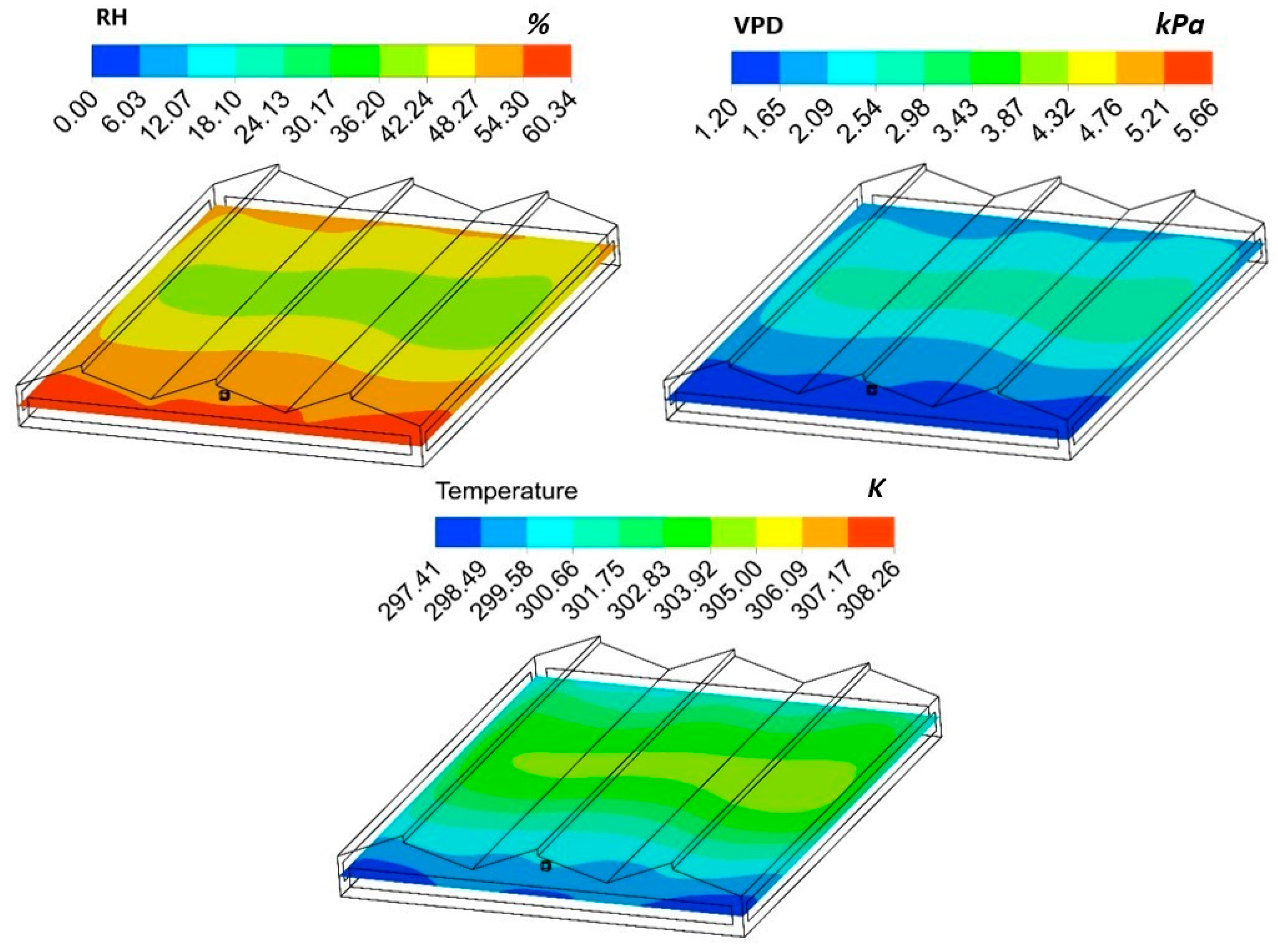
3.2. Analysis of the Results of Simulated Scenarios

The environmental analysis of the simulated scenarios was performed on the basis of the concentration of water vapor in the air, temperature, NIR, and vapor pressure deficit (VPD)—indicators used to manage the greenhouse environment and maintain suitable conditions for growing tomatoes within it. The analysis of the influence of concentration of the water vapor on the temperature was limited to measurements at the center of each span; in contrast, simulated data were computed as averages along the greenhouse, away from the predominant air inlet in the greenhouse. In each simulated scenario, a dataset of 100 data points was obtained longitudinally at a height of 1.5 m and was used for the environmental analysis shown in Figure 3. These distances were selected for the analysis because the central span was characterized by greater thermal and humidity gradients in the air between the windward and leeward zones. The results in Figure 3 show a decrease in temperature in relation to the increase in water vapor concentration in the simulated scenarios. The thermal gradient range in the greenhouse (length) was around 2 °C in the crop zone (1.5 m height), being remarkable in the first half of the greenhouse. In the area near the outlet, the thermal gradient range was negligible (0.15 °C) between scenarios a, b, and c.

On the other hand, for the VPD along the greenhouse length, there was a 2 kPa difference between scenarios, and this remained constant. This finding was derived from the influence on temperature (T) and relative humidity (RH) from external local climate conditions. In addition, for crop simulations, enhanced environmental conditions favoring crop growth were observed inside the greenhouse. We concluded that the most significant change occurred in the first half of the greenhouse. In the area near the outlet, the increase in water vapor concentration did not influence the increase in temperature.

To calculate the VPD in the greenhouse, the equation was programmed with a user-defined function (UDF) in CFD. The VPD value was estimated as the difference between the saturation vapor pressure value and the actual vapor pressure of the air (VPD = PVsat − Pvair), a method recommended by Howell and Dusek, and FAO [58,59]. The greenhouse analysis was performed in all the simulated scenarios as an average of 10 data points uniformly distributed within a height range of 1.9–2 m at the inlet, center, and outlet of the central span. The results in

Table 6. Average of ten data of the variables: T, RH, and VPD simulated at a height from 1.9 to 2 m at the inlet, center, and outlet area of the central span of the greenhouse.

Position	Scenario	T (°C)	RH (%)	VPD (kPa)
Inlet	a	32.94	25.68	3.73
	b	33.10	36.15	3.23
	c	33.23	45.49	2.78
Center	a	34.83	23.11	4.28
	b	34.92	32.67	3.77
	c	34.99	41.24	3.30
Outlet	a	34.70	23.29	4.24
	b	34.77	32.93	3.72
	c	34.85	41.56	3.26

show the spatial variation in the water vapor concentration and thermal gradient at three points of observation along the length of the greenhouse.

The temperature increase was generated from the absorption of NIR by water vapor; however, when the mass fraction of water vapor remains constant in the air at the center and outlet areas of the greenhouse, the RH gradient is minimal equal to 0.78%. Therefore, the thermal effect generated by the energy exchange between water vapor and NIR is negligible. In all scenarios, there is a reduction between the outside RH and that of the greenhouse with a gradient that ranges between 45 and 50% caused by the low speed of the outside wind (0.64 m s⁻¹) and the anti-insect mesh in the windows.

The increase in temperature inside the greenhouse, given the increase in water vapor concentration in the air, was not significant, ranging from 0.15 to 0.28 °C (Table 6). For this reason, it was inferred that the temperature remained constant under the simulated conditions and was not influenced by the variation in the mass fraction of water vapor.

The simulation of scenario b was carried out with a change in the intensity emitted by the NIR (50 and 100 W m⁻²) to analyze the effect it had on temperature. The results of the simulations (

Table 7. Climate variation with a change in NIR intensity for scenario b.

Position	Scenario	T (°C)	RH (%)	VPD (kPa)	NIR (W m−2)
Inlet	b1	32.97	36.42	3.19	60.46
	b	33.02	36.31	3.21	120.91
	b2	33.10	36.15	3.23	189.98
Center	b1	34.75	32.97	3.72	66.33
	b	34.82	32.85	3.74	132.67
	b2	34.92	32.67	3.77	195.94
Outlet	b1	34.59	33.26	3.67	68.45
	b	34.66	33.13	3.69	136.91
	b2	34.77	32.93	3.72	198.69

) show that when there was a change in the intensity of NIR, the highest thermal gradient (0.23 °C) occurred at the inlet and outlet areas of span 2 of the greenhouse, where the wind speeds were below 0.01 m s⁻¹ and air movement was generated by the convective effect caused by temperature differences. This was also demonstrated by Sun et al., and Zeroual et al. [3,7], where outside wind speeds close to 1 m s⁻¹ were insufficient to renew the air inside the greenhouse, affecting the exchange of heat and mass between the outside and the inside.

Derived from the change in the concentration of the mass fraction of water vapor and the NIR intensity in the simulated scenarios, the highest thermal gradient occurred in the inlet area (0.29 °C), where the RH of the greenhouse was higher due to the air exchange between outside and inside. Therefore, it could be assumed that the generated temperature gradient was negligible, as in most of the greenhouse it oscillated between 0.08–0.16 °C.

Figure 4 shows the distribution of RH and VPD inside the greenhouse in the simulated scenarios at a height of 1.5 m. The results indicate that scenario c presented better environmental conditions for tomato cultivation with lower VPD (kPa), temperature T (°C), and higher RH (%) inside the greenhouse. Nevertheless, there was a 53% reduction in RH between the outside and inside of the greenhouse, causing this scenario to be outside the desirable optimum for tomato (50–60%) [60]. The RH deficit inside the greenhouse caused an increase in the VPD, with values over 1.3 kPa for all simulated scenarios, values outside the range for tomato (0.3–1.25 kPa) according to Grange et al., Körner et al. and Shtienberg [15,61,62]. The VPD values in Figure 4 show that under the conditions of the simulated scenarios, the crop inside the greenhouse would undergo a high rate of transpiration, causing the closure of its stomata and impeding its growth [14].

Scenario b was simulated with the mean monthly wind speed (1.59 m s⁻¹) during the month of February in Montecillo, Mexico according to data from the National Meteorological Service (SMN). The purpose of the simulation under these conditions was to predict the effects on environmental conditions that can occur when wind speed increases. These changes were simulated, and the results in Figure 5 show enhanced environmental conditions for tomato crop cultivation compared to the scenario b of Figure 4 with decreases in temperature and VPD that oscillated between 4–6 °C and 0.9–1.63 kPa, respectively. Likewise, it presents an increase in RH of between 8.3–15.4% throughout the greenhouse. However, these generated changes were not enough to maintain a RH between 50–60%, a temperature below 30 °C, and a VPD between 0.3–1.25 kPa throughout the greenhouse.

The results of the simulations carried out in this work also confirm what was described by Chu, Lan, Tasi, Wu, and Yang; and Tong et al. [46,63], where lengths greater than six times the height of the greenhouse present problems in the ventilation rate due to the obstruction generated by the anti-insect mesh and the length of the greenhouse. Therefore, the use of fans and extractors is recommended to avoid stagnant areas in the center of greenhouse buildings when natural ventilation is insufficient to improve the ventilation rate [9,10,64].

4. Conclusions

The greenhouse air inlet area was the location with the highest energy exchange in all of the simulated scenarios, with a temperature increase of 0.29 °C generated by the absorption of NIR and by the exchange of air between the outside and inside. The greenhouse scenarios did not present favorable environmental conditions for tomato cultivation. The temperature exceeded 30 °C with an average thermal gradient between the outside and inside of up to 12 °C, causing an RH deficit and an increase in VPD to values higher than 2 kPa, which consequently would cause excess perspiration in tomato and an expected stomatal closure. The temperature gradient between the outside and inside of the greenhouse was the result of the low wind speed (0.64 m s⁻¹) and the anti-insect mesh, causing air movement within the greenhouse to be generated by the difference between soil and air temperatures. Environmental conditions improved when the scenario was simulated with the monthly mean wind speed for the month of February (1.59 m s⁻¹) in Texcoco; however, this was not enough to maintain favorable environmental conditions. From this, it is inferred that natural ventilation is insufficient to reduce the thermal gradient and increase the RH to acceptable values for tomato. Therefore, the use of fans and extractors is recommended to increase the exchange of heat and mass between the outside and inside and help to distribute the RH and temperature evenly in the stagnant area of the greenhouse (in the center of the spans).

References

1. Liu, J.Q.; Yin, C.; Zhao, H.D. Ventilation management of solar greenhouse. Vegetables 2003, 2, 33–34. [Google Scholar]
2. Molina-Aiz, F.D.; Valera, D.L.; Peña, A.A.; Gil, J.A.; López, A. A study of natural ventilation in an Almería-type greenhouse with insect screens by means of tri sonic anemometry. Biosyst. Eng. 2009, 104, 224–242. [Google Scholar] [CrossRef]
3. Sun, M.; Luo, W.H.; Feng, W.L.; Xiang, L.; Fu, X.G. A web-based expert system for diagnosis and control management of diseases in vegetable crops cultivated under protected conditions. J. Nanjing Agric. Univ. 2014, 37, 7–14. [Google Scholar]
4. Cemek, B.; Atiş, A.; Küçüktopçu, E. Evaluation of temperature distribution in different greenhouse models using computational fluid dynamics (CFD). Anadolu J. Agric. Sci. 2017, 32, 54–63. [Google Scholar] [CrossRef] [Green Version]
5. Teitel, M.; Liran, O.; Tanny, J.; Barak, M. Wind driven ventilation of a mono-span greenhouse with a rose crop and continuous screened side vents and its effect on flow patterns and microclimate. Biosyst. Eng. 2008, 101, 111–122. [Google Scholar] [CrossRef]
6. Rico-Garcia, E.; Soto-Zarazua, G.; Alatorre-Jacome, O.; De la Torre-Gea, G.A.; Gomez-Melendez, D.J. Aerodynamic study of greenhouses using computational fluid dynamics. Int. J. Phys. Sci. 2011, 6, 6541–6547. [Google Scholar] [CrossRef]
7. Zeroual, S.; Bougoul, S.; Benmoussa, H. Effect of radiative heat transfer and boundary conditions on the airflow and temperature distribution inside a heated tunnel greenhouse. J. Appl. Mech. Tech. Phys. 2018, 59, 1008–1014. [Google Scholar] [CrossRef]
8. Fidaros, D.; Baxevanou, C.A.; Bartzanas, T.; Kittas, C. Numerical simulation of thermal behavior of a ventilated arc greenhouse during a solar day. Renew. Energy 2010, 35, 1380–1386. [Google Scholar] [CrossRef]
9. Teitel, M.; Wenger, E. Air exchange and ventilation efficiencies of a monospan greenhouse with one inflow and one outflow through longitudinal side openings. Biosyst. Eng. 2014, 119, 98–107. [Google Scholar] [CrossRef]
10. Bournet, P.; Boulard, T. Effect of ventilator configuration on the distributed climate of greenhouses: A review of experimental and CFD studies. Comput. Electron. Agric. 2010, 74, 195–217. [Google Scholar] [CrossRef]
11. Fernandez, M.; Orgaz, F.; Fereres, E.; Lopez, J.; Cespedes, A.; Perez, J.; Bonachela, S.; Gallardo, M. Programación del Riego de Cultivos Hortícolas Bajo Invernadero en el Sudeste Español; Fundacion CAJAMAR. Caja Rural de Almería y Málaga: Barcelona, Spain, 2001; p. 71. [Google Scholar]
12. Prenger, J.; Ling, P. Greenhouse condensation control, understanding and using vapor pressure deficit (VPD). Extension FactSheet; Ohio State University Extension Fact Sheet: Columbus, OH, USA, 2001; p. 4. [Google Scholar]
13. Dik, A.; Wubben, J. Epidemiology of Botrytis cinerea diseases in greenhouses. In Biology, Pathology and Control, 2nd ed.; Elad, Y., Williamson, B., Tudzynsky, P., Delen, N., Eds.; Springer: Dordrecht, The Netherlands, 2001; pp. 319–331. [Google Scholar]
14. Lopez, J. Control Climático en Invernaderos, 1st ed.; Novedades agrícolas: Murcia, Spain, 2005; p. 4. [Google Scholar]
15. Shtienberg, D. Rational management of Botrytis-incited diseases: Integration of control measures and use of warning systems. In Biology, Pathology and Control, 2nd ed.; Elad, Y., Williamson, B., Tudzynsky, P., Delen, N., Eds.; Springer: Dordtrecht, The Netherlands, 2007; pp. 335–346. [Google Scholar]
16. Beluzán, J. Déficit de presión de vapor (DPV) y factores microclimáticos como herramientas de pronóstico de Botrytis cinerea Pers. ex Fr., en Lactuca sativa L. bajo invernadero. Master’ Thesis, Universidad Austral de Chile Facultad de Ciencias Agrarias, Valdivia, Chile, 2013. [Google Scholar]
17. Baxevanou, C.; Fidaros, D.; Bartzanas, T.; Kittas, C. Numerical simulation of solar radiation, air flow and temperature distribution in a naturally ventilated tunnel greenhouse. Agric. Eng. Int. CIGR J. 2010, 12, 48–67. [Google Scholar]
18. Sethi, V.P.; Sharma, S.K. Thermal modeling of a greenhouse integrated to an aquifer coupled cavity flow heat exchanger system. Sol. Energy 2007, 81, 723–741. [Google Scholar] [CrossRef]
19. Mesmoudi, K.; Meguallati, K.H.; Bournet, P.E. Effect of the greenhouse design on the thermal behavior and microclimate distribution in greenhouses installed under semi-arid climate. Heat Transf. Asian Res. 2017, 46, 1294–1311. [Google Scholar] [CrossRef]
20. Kendirli, B. Structural analysis of greenhouses: A case study in Turkey. Build. Environ. 2006, 41, 864–871. [Google Scholar] [CrossRef]
21. Stanciu, C.; Stanciu, D.; Dobrovicescu, A. Effect of greenhouse orientation with respect to E-W axis on its required heating and cooling loads. Energy Procedia 2016, 85, 498–504. [Google Scholar] [CrossRef] [Green Version]
22. Mobtaker, H.G.; Ajabshirchi, Y.; Ranjbar, S.F.; Matloobi, M. Simulation of thermal performance of solar greenhouse in north-west of Iran: An experimental validation. Renew. Energy 2018, 135, 88–97. [Google Scholar] [CrossRef]
23. Geoola, F.; Kashti, Y.; Peiper, U.M. A model greenhouse for testing the role of condensation, dust and dirt on the solar radiation. J. Agric. Eng. Res. 1998, 71, 339–346. [Google Scholar] [CrossRef]
24. Kindelan, M. Dynamic modelling of greenhouse environment. Trans. ASAE 1980, 23, 1232–1239. [Google Scholar] [CrossRef]
25. Bot, G.P.A. Greenhouse Climate: From Physical Processes to a Dynamic Model. Ph.D. Thesis, Agricultural University of Wageningen, Wageningen, The Netherlands, 1983. [Google Scholar]
26. Molina-Aiz, F.D.; Valera, D.L.; Álvarez, A.J. Measurement and simulation of cli- mate inside Almerıa-type greenhouses using computational fluid dynamics. Agric. For. Meteorol. 2004, 125, 33–51. [Google Scholar] [CrossRef]
27. Campen, J.B.; Bot, G.P.A. Determination of greenhouse-specific aspects of ventilation using three-dimensional computational fluid dynamics. Biosyst. Eng. 2003, 84, 69–77. [Google Scholar] [CrossRef]
28. Miller, G.T. Ciencia Ambiental: Preservemos la Tierra, 5th ed.; Thomson: Belmont, Australia, 2002; p. 456. [Google Scholar]
29. Nebel, B.J.; Wright, R.T. Ciencias ambientales: Ecología y desarrollo sostenible, 6th ed.; Pearson Educación: London, UK, 1999; p. 69. [Google Scholar]
30. Collins, W.D.; Lee-Taylor, J.M.; Edwards, D.P.; Francis, G.L. Effects of increased near-infrared absorption by water vapor on climate system. J. Geophys. Res. 2006, 111. [Google Scholar] [CrossRef] [Green Version]
31. Kiehl, J.T.; Trenberth, K.E. Earth’s annual global mean energy budget. Bull. Am. Meteorol. Soc. 1997, 78, 197–208. [Google Scholar] [CrossRef] [Green Version]
32. Ramaswamy, V.; Freidenreich, S.M. Solar radiative line-by-line determination of water vapor absorption and water cloud extinction in inhomogeneous atmospheres. J. Geophys. Res. 1991, 96, 9133–9157. [Google Scholar] [CrossRef]
33. Bournet, P.E.; Ould-Khaoua, S.A.; Boulard, T. Numerical prediction of the effect of vents arrangement on the ventilation and energy transfer in a multispan glasshouse using a bi-band radiation model. Biosyst. Eng. 2007, 98, 224–234. [Google Scholar] [CrossRef]
34. Kim, K.; Yoon, J.; Kwon, H.; Han, J.; Son, J.E.; Nam, S.; Giacomelli, G.; Lee, I. 3-D CFD analysis of relative humidity distribution in greenhouse with a fog cooling system and refrigerative dehumidifiers. Biosyst. Eng. 2008, 100, 245–255. [Google Scholar] [CrossRef]
35. Wang, X.W.; Luo, J.Y.; Li, X.P. CFD based study of heterogeneous microclimate in a typical chinese greenhouse in central China. J. Integr. Agric. 2013, 12, 914–923. [Google Scholar] [CrossRef]
36. Chen, J.; Xu, F.; Tan, D.; Shen, Z.; Zhang, L.; Ai, Q. A control method for agricultural greenhouses heating based on computational fluid dynamics and energy prediction model. Appl. Energy 2015, 141, 106–118. [Google Scholar] [CrossRef]
37. Kichah, A.; Bournet, P.E.; Migeon, C.; Boulard, T. Measurements and CFD simulations of microclimate characteristics and transpiration of an Impatiens pot plant crop in a greenhouse. Biosyst. Eng. 2012, 112, 22–34. [Google Scholar] [CrossRef]
38. Nebbali, R.; Roy, J.C.; Boulard, T. Dynamic simulation of the distributed radiative and convective climate within a cropped greenhouse. Renew. Energy 2012, 43, 111–129. [Google Scholar] [CrossRef]
39. Morille, B.; Migeon, C.; Bournet, P.E. Is the Penmane-Monteith model adapted to predict crop transpiration under greenhouse conditions? Application to a New Guinea Impatiens crop. Sci. Hortic. 2013, 152, 80–91. [Google Scholar] [CrossRef]
40. Roy, J.C.; Pouillard, J.B.; Boulard, T.; Fatnassi, H.; Grisey, A. Experimental and CFD results on the CO2 distribution in a semi-closed greenhouse. Acta Hortic. 2014, 1037, 993–1000. [Google Scholar] [CrossRef]
41. Boulard, T.; Roy, J.C.; Pouillard, J.B.; Fatnassi, H.; Grisey, A. Modelling of micrometeorology, canopy transpiration and photosynthesis in a closed greenhouse using computational fluid dynamics. Biosyst. Eng. 2017, 158, 110–133. [Google Scholar] [CrossRef]
42. Majdoubi, H.; Boulard, T.; Fatnassi, H.; Bouirden, L. Airflow and microclimate patterns in a one-hectare Canary type greenhouse: An experimental and CFD assisted study. Agric. For. Meteorol. 2009, 149, 1050–1062. [Google Scholar] [CrossRef]
43. Sethi, V.P. On the selection of shape and orientation of a greenhouse: Thermal modeling and experimental validation. Sol. Energy 2009, 83, 21–38. [Google Scholar] [CrossRef]
44. Baxevanou, C.; Fidaros, D.; Bartzanas, T.; Kittas, C. Yearly numerical evaluation of greenhouse cover materials. Comput. Electron. Agric. 2018, 149, 54–70. [Google Scholar] [CrossRef]
45. Muñoz, P.; Montero, J.; Anton, A.; Iglesias, N. Computational fluid dynamic modelling of night-time energy fluxes in unheated greenhouses. Acta Hortic. 2004, 691, 403–410. [Google Scholar]
46. Tong, G.; Christopher, D.; Li, T.; Wang, T. Passive solar energy utilization: A review of cross-section building parameter selection for Chinese solar greenhouses. Renew. Sustain. Energy Rev. 2013, 26, 540–548. [Google Scholar] [CrossRef]
47. Bartzanas, T.; Boulard, T.; Kittas, C. Effect of vent arrangement on windward ventilation of a tunnel greenhouse. Biosyst. Eng. 2004, 88, 479–490. [Google Scholar] [CrossRef]
48. Lamnatou, C.; Chemisana, D. Solar radiation manipulations and their role in greenhouse claddings: Fresnel lenses, NIR- and UV-blocking materials. Renew. Sustain. Energy Rev. 2013, 18, 271–287. [Google Scholar] [CrossRef]
49. Stanghellini, C.; Dai, J.; Kempkes, F. Effect of near-infrared-radiation reflective screen materials on ventilation requirement, crop transpiration and water use efficiency of a greenhouse rose crop. Biosyst. Eng. 2011, 110, 261–271. [Google Scholar] [CrossRef]
50. Murakami, K.; Fukuoka, N.; Noto, S. Improvement of greenhouse microenvironment and sweetness of melon (Cucumis melo L.) fruits by greenhouse shading with a new kind of near-infrared ray-cutting net in mid-summer. Sci. Hortic. 2017, 218, 1–7. [Google Scholar] [CrossRef]
51. Rosenberg, N.J.; Blad, B.L.; Verma, S.B. Microclimate: The Biological Environment, 2nd ed.; John Wiley and Sons: Hoboken, NJ, USA, 1983; p. 495. [Google Scholar]
52. Senhaji, A.; Majdoubi, H.; Mouqalid, M.; De, E.; Meknès, E. Solar distribution in a greenhouse at different crops orientation during production season. In Proceedings of the 13ème Congrès Mécanique, Meknes, Morocco, 11–14 April 2017; pp. 13–15. [Google Scholar]
53. Aguilar-Rodriguez, C.E.; Flores-Velazquez, J.; Ojeda-Bustamante, W.; Rojano, F.; Iñiguez-Covarrubias, M. Valuation of the energy performance of a greenhouse with an electric heater using numerical simulations. Processes 2020, 8, 600. [Google Scholar] [CrossRef]
54. Bouhoun-Ali, H.; Bournet, P.E.; Cannavo, P.; Chantoiseau, E. Development of a CFD crop submodel for simulating microclimate and transpiration of ornamental plants grown in a greenhouse under water restriction. Comput. Electron. Agric. 2017, 149, 26–40. [Google Scholar] [CrossRef]
55. Launder, B.E.; Spalding, D.B. Lectures in Mathematical Models of Turbulence; Academic Press: London, UK, 1972. [Google Scholar]
56. Launder, B.E.; Spalding, D.B. The numerical computation of turbulent flows. Comput. Methods Appl. Mech. Eng. 1974, 3, 269–289. [Google Scholar] [CrossRef]
57. Bouhoun-Ali, H.; Bournet, P.E.; Danjou, V.; Morille, B.; Migeon, C. CFD simulations of the night-time condensation inside a closed glasshouse: Sensitivity analysis to outside external conditions, heating and glass properties. Biosyst. Eng. 2014, 127, 159–175. [Google Scholar] [CrossRef]
58. Howell, T.; Dusek, D. Comparison of vapor pressure deficit calculation methods, southern high plains. J. Irrig. Drain. Eng. 1995, 121, 191–198. [Google Scholar] [CrossRef]
59. Food Agricultural Organization (FAO). Evapotranspiración del Cultivo; FAO: Rome, Italy, 2006; p. 298. [Google Scholar]
60. Huerres, P.C.; Caraballo, N. Horticultura; Editorial Pueblo y Educación: La Habana, Cuba, 1988; p. 193. [Google Scholar]
61. Grange, R.; Hand, D. A review of the effects of atmospheric humidity on the growth of horticultural crops. J. Hortic. Sci. 1987, 62, 125–134. [Google Scholar] [CrossRef]
62. Körner, O.; Challa, H. Process-based humidity control regime for greenhouse crops. Comp. Electr. Agric. 2003, 39, 173–192. [Google Scholar] [CrossRef]
63. Chu, C.R.; Lan, T.W.; Tasi, R.K.; Wu, T.R.; Yang, C.K. Wind-driven natural ventilation of greenhouses with vegetation. Biosyst. Eng. 2017, 164, 221–234. [Google Scholar] [CrossRef]
64. Flores-Velázquez, J.; Villarreal-Guerrero, F. Design of a forced ventilation system for a Zenithal greenhouse using CFD. Rev. Mex. De Cienc. Agrícolas 2015, 6, 303–316. [Google Scholar]
Figure 1. Dimensions and distribution of the heater () and the temperature (), humidity (), and eddy covariance system () sensors in the three spans of the experimental greenhouse.
Processes 09 01587 g001
Figure 2. Spatial variation in temperature from 2:00 p.m. to 2:30 p.m.
Processes 09 01587 g002
Figure 3. (A) Temperature distribution (°C) and (B) VPD (kPa) for the simulated scenarios along the length of greenhouse at 1.5 m height. The three scenarios a, b and c, and simulating the incorporation of a tomato crop to develop LAI 3.5.
Processes 09 01587 g003
Figure 4. Distribution of RH (%) and VPD (kPa) in the greenhouse at 1.5 m height in the simulations for the three scenarios (ac) specified in Table 6.
Processes 09 01587 g004
Figure 5. Distribution of RH (%), temperature (K), and VPD (kPa) in the greenhouse at 1.5 m height in scenario b, considering the mean monthly wind speed (1.59 m s−1) during February.
Processes 09 01587 g005