Article

An Improved Hybrid Aquila Optimizer and Harris Hawks Algorithm for Solving Industrial Engineering Optimization Problems

1
School of Information Engineering, Sanming University, Sanming 365004, China
2
Research and Innovation Department, Skyline University College, Sharjah 1797, United Arab Emirates
3
Faculty of Computer Sciences and Informatics, Amman Arab University, Amman 11953, Jordan
4
School of Computer Science, Universiti Sains Malaysia, Gelugor 11800, Pulau Pinang, Malaysia
5
School of Computer Science and Technology, Hainan University, Haikou 570228, China
*
Author to whom correspondence should be addressed.
Processes 2021, 9(9), 1551; https://doi.org/10.3390/pr9091551
Submission received: 20 July 2021 / Revised: 26 August 2021 / Accepted: 27 August 2021 / Published: 30 August 2021
(This article belongs to the Special Issue Evolutionary Process for Engineering Optimization)

Abstract

:
Aquila Optimizer (AO) and Harris Hawks Optimizer (HHO) are recently proposed meta-heuristic optimization algorithms. AO possesses strong global exploration capability but insufficient local exploitation ability. However, the exploitation phase of HHO is pretty good, while the exploration capability is far from satisfactory. Considering the characteristics of these two algorithms, an improved hybrid AO and HHO combined with a nonlinear escaping energy parameter and random opposition-based learning strategy is proposed, namely IHAOHHO, to improve the searching performance in this paper. Firstly, combining the salient features of AO and HHO retains valuable exploration and exploitation capabilities. In the second place, random opposition-based learning (ROBL) is added in the exploitation phase to improve local optima avoidance. Finally, the nonlinear escaping energy parameter is utilized better to balance the exploration and exploitation phases of IHAOHHO. These two strategies effectively enhance the exploration and exploitation of the proposed algorithm. To verify the optimization performance, IHAOHHO is comprehensively analyzed on 23 standard benchmark functions. Moreover, the practicability of IHAOHHO is also highlighted by four industrial engineering design problems. Compared with the original AO and HHO and five state-of-the-art algorithms, the results show that IHAOHHO has strong superior performance and promising prospects.

1. Introduction

Meta-heuristic optimization algorithms inspired by nature are becoming more and more popular in real-world applications [1]. Meta-heuristics usually mimic biological or physical phenomena and only consider inputs and outputs, making them flexible and straightforward. Furthermore, meta-heuristics is a kind of stochastic optimization technique. This property assists them to effectively avoid local optima, which usually occurs in real problems. Because of the advantages of simplicity, flexibility, and ability to avoid local optima, meta-heuristic optimization algorithms outperform heuristic optimization algorithms to solve various complex and tricky optimization problems in the real world [2].
Three dominant categories are divided from meta-heuristic optimization algorithms: evolutionary, physics-based, and swarm intelligence techniques. Evolutionary algorithms are inspired by the laws of evolution in nature. The randomly generated population evolves over subsequent generations as the number of iterations increases. Each generation of individuals is always formed by the combination of best individuals so that the population can be optimized over several generations of evolution. The most popular evolutionary technique is Genetic Algorithms (GA) [3], which simulates Darwin’s theory of evolution. There are several other popular evolutionary algorithms, such as Differential Evolution Algorithm (DE) [4], Genetic Programming (GP) [5], Evolution Strategy (ES) [6], Biogeography-Based Optimizer (BBO) [7], Evolutionary Deduction Algorithm (ED) [8], and Probability-Based Incremental Learning (PBIL) [9]. Physics-based methods are inspired by the physical rules of the universe. The most popular algorithms in this category are Simulated Annealing (SA) [10], Big-Bang Big-Crunch (BBBC) [11], Gravity Search Algorithm (GSA) [12], Gravitational Local Search (GLSA) [13], Heat Transfer Relation-based Optimization Algorithm (HTOA) [14], Charged System Search (CSS) [15], Artificial Chemical Reaction Optimization Algorithm (ACROA) [16], Central Force Optimization (CFO) [17], Ray Optimization (RO) [18] algorithm, Black Hole (BH) [19] algorithm, Small-World Optimization Algorithm (SWOA) [20], Galaxy-based Search Algorithm (GbSA) [21], Curved Space Optimization (CSO) [22], Multi-Verse Optimizer (MVO) [23], Sine Cosine Algorithm (SCA) [24], and Arithmetic Optimization Algorithm (AOA) [25].
The third category is swarm intelligence algorithms, which simulate the behaviour of swarms of creatures in nature. The most well-known swarm intelligence technique is Particle Swarm Optimization (PSO), first proposed by Kennedy and Eberhart [26]. PSO mimics the behaviour of bird flocks in navigating and foraging, and the birds achieve the optimal position through collective cooperation. Particles update positions not only considering their own best positions but also according to the best position of the swarm obtained so far. Other representative algorithms include Ant Colony Optimization Algorithm (ACO) [27], Monkey Search [28], Firefly Algorithm [29], Bat Algorithm (BA) [30], Krill Herd (KH) [31], Grey Wolf Optimizer (GWO) [32], Cuckoo Search (CS) Algorithm [33], Fruit Fly Optimization (FFO) [34], Dolphin Partner Optimization (DPO) [35], Ant Lion Optimizer (ALO) [36], Remora Optimization Algorithm (ROA) [37], Whale Optimization Algorithm (WOA) [38], Salp Swarm Algorithm (SSA) [39], Bald Eagle Search (BES) algorithm [40], and Slime Mould Algorithm (SMA) [41].
As one of the swarm intelligence algorithms, the Harris Hawks Optimizer (HHO) [42] was proposed in 2019. HHO simulates several hunting strategies of Harris’s hawk and attracted several researchers to apply it to solve practical problems [43,44,45,46,47]. The exploitation phase of HHO includes four strategies, but the exploration phase is insufficient, and the balance between the exploration and exploitation phases is not good enough. Therefore, many improved and hybrid researches have been proposed to enhance the performance of HHO. Yousri et al. [48] proposed an enhanced algorithm based on the fractional calculus (FOC) memory concept to improve the performance of exploration phase, which is known as FMHHO. The hawk moves with a fractional-order velocity, and the escaping energy of the prey is adaptively adjusted based on FOC parameters to avoid local optima stagnation. Gupta et al. [49] introduced a nonlinear energy parameter, different settings for rapid dives, opposition-based learning strategy, and a greedy selection mechanism into HHO to enhance the search efficiency and avoid premature convergence. Hussien and Amin [50] proposed an improved HHO called IHHO to enhance the performance of HHO. The proposed IHHO applied opposition-based learning (OBL) in the initialization phase to diverse the initial population as well as Chaotic Local Search (CLS) strategy and a self-adaptive technique to improve its performance and speed up the convergence of the algorithm. Sihwail et al. [51] proposed a new search mechanism and then applied it and elite opposite-based learning (EOBL) technique to HHO. The improved HHO raised the search capabilities by mutation, mutation neighborhood search (MNS), and rollback strategy. It can avoid local optimum entrapment and improve population diversity, convergence accuracy, and rate. Bao et al. [52] proposed HHO-DE by hybridizing HHO and Differential Evolution (DE) algorithms. HHO and DE were used to update the positions of two equal subpopulations respectively. The proposed HHO-DE has high accuracy, ability to avoid local optima, and remarkable stability. Houssein et al. [53] combined HHO with cuckoo search (CS) and chaotic maps to propose a hybrid algorithm called CHHO-CS. CS was used to control the main position vectors of HHO to achieve a better balance between exploration and exploitation phases, and chaotic maps were adopted to update the control energy parameters to avoid premature convergence. Kaveh et al. [54] proposed an effective algorithm called ICHHO by hybridizing HHO with Imperialist Competitive Algorithm (ICA). Combination of the exploration strategy of ICA and exploitation technique of HHO helps to achieve a better search strategy. These improved and hybrid algorithms have proven that HHO is a valuable algorithm. Aquila Optimizer (AO) [55] is the latest swarm intelligence algorithm, proposed in 2021. This algorithm simulates different hunting methods of Aquila for different kinds of prey. The hunting methods for fast-moving prey reflect the global exploration ability of the algorithm, and the hunting methods for slow-moving prey reflect the local exploitation ability of the algorithm. AO algorithm possesses strong global exploration ability, high search efficiency, and fast convergence speed, but its local exploitation ability is insufficient, so it is easy to fall into local optima. Due to the short time that has elapsed since the algorithm has been proposed, there is no research on the improvement of AO yet.
Therefore, we tried a kind of hybridization to improve the performance of HHO and AO. As far as we know, this kind of hybridization of HHO with AO has not been used before. We propose a new, improved hybrid Aquila Optimizer and Harris Hawks Optimization (IHAOHHO) by combining the salient features of AO and HHO. In this paper, we integrate the exploitation strategy of HHO into the AO algorithm, which is added random opposition-based learning (ROBL) in the exploitation phase to avoid local optima stagnation. At the same time, the nonlinear escaping energy parameter balances the exploration and exploitation phases of the algorithm. The 23 standard benchmark functions and four engineering design problems were applied to test the exploration and exploitation capabilities of IHAOHHO. The proposed algorithm is compared with original AO, HHO, and several well-known algorithms, including SMA, SSA, WOA, GWO, and PSO. The experimental results show that the proposed IHAOHHO algorithm performs better than the state-of-the-art meta-heuristic algorithms.
The rest of this paper is organized as follows (Figure 1): Section 2 provides a brief overview of the related work: original Harris Hawks Optimization algorithm and Aquila Optimizer, as well as two improvement strategies. Section 3 describes in detail the proposed hybrid algorithm. Section 4 conducts simulation experiments and results analysis. Finally, Section 5 concludes the paper.

2. Preliminaries

2.1. Aquila Optimizer (AO)

AO is a latest novel swarm intelligence algorithm proposed by Abualigah et al. in 2021. There are four hunting behaviors of Aquila for different kinds of prey. Aquila can switch hunting strategies flexibly for different prey and then uses its fast speed united with sturdy feet and claws to attack prey. The brief description of mathematical model can be described as follows.
Step 1:
Expanded exploration (X1): high soar with a vertical stoop
In this method, the Aquila flies high over the ground and explores the search space widely, and then a vertical dive is taken once the Aquila determines the area of the prey. The mathematical representation of this behaviour is written as:
X 1 ( t + 1 ) = X b e s t ( t ) × ( 1 t T ) + ( X M ( t ) X b e s t ( t ) × r 1 )
X M ( t ) = 1 N i = 1 N X i ( t )
where X b e s t ( t ) represents the best position obtained so far, and X M ( t ) denotes the average position of all Aquilas in current iteration. t and T is the current iteration and the maximum number of iterations, respectively. N is the population size, and r 1 is a random number between 0 and 1.
Step 2:
Narrowed exploration (X2): contour flight with short glide attack
This is the most commonly used hunting method for Aquila. It uses short gliding to attack the prey after descending within the selected area and flying around the prey. The position update formula is represented as:
X 2 ( t + 1 ) = X b e s t ( t ) × L F ( D ) + X R ( t ) + ( y x ) × r 2
where X R ( t ) represents a random position of the Aquila, D is the dimension size, and r 2 is a random number within (0, 1). L F ( D ) represents Levy flight function, which is presented as follows:
L F ( D ) = s × u × σ | v | 1 β
σ = Γ ( 1 + β ) × sin ( π β 2 ) Γ ( 1 + β 2 ) × β × 2 ( β 1 2 )
where s and β are constant values equal to 0.01 and 1.5, respectively, and u and v are random numbers between 0 and 1. y and x are used to present the spiral shape in the search, which are calculated as follows:
x = r × sin ( θ ) y = r × cos ( θ ) r = r 3 + 0.00565 × D 1 θ = ω × D 1 + 3 × π 2
where r 3 means the number of search cycles between 1 and 20, D 1 is composed of integer numbers from 1 to the dimension size ( D ), and ω is equal to 0.005.
Step 3:
Expanded exploitation (X3): low flight with a slow descent attack
In the third method, when the area of prey is roughly determined, the Aquila descends vertically to do a preliminary attack. AO exploits the selected area to get close and attack the prey. This behaviour is presented as follows:
X 3 ( t + 1 ) = ( X b e s t ( t ) X M ( t ) ) × α r 4 + ( ( U B L B ) × r 5 + L B ) × δ
where X b e s t ( t ) denotes to the best position obtained so far, and X M ( t ) means the average value of the current positions. α and δ are the exploitation adjustment parameters fixed to 0.1, U B and L B are the upper and lower bound of the problem, and r 4 and r 5 are random numbers within (0, 1).
Step 4:
Narrowed exploitation (X4): walking and grabbing prey
In this method, the Aquila chases the prey in the light of its escape trajectory and then attacks the prey on the ground. The mathematical representation of this behaviour is as follows:
X 4 ( t + 1 ) = Q F × X b e s t ( t ) ( G 1 × X ( t ) × r 6 ) G 2 × L F ( D ) + r 7 × G 1 Q F ( t )   = t 2 × r a n d ( ) 1 ( 1 T ) 2 G 1 = 2   × r 8 1 G 2 = 2   × ( 1 t T )
where X ( t ) is the current position, and Q F ( t ) represents the quality function value, which used to balance the search strategy. G 1 denotes the movement parameter of Aquila during tracking prey, which is a random number between [–1,1]. G 2 denotes the flight slope when chasing prey, which decreases linearly from 2 to 0. r 6 , r 7 , and r 8 are random numbers between 0 and 1.

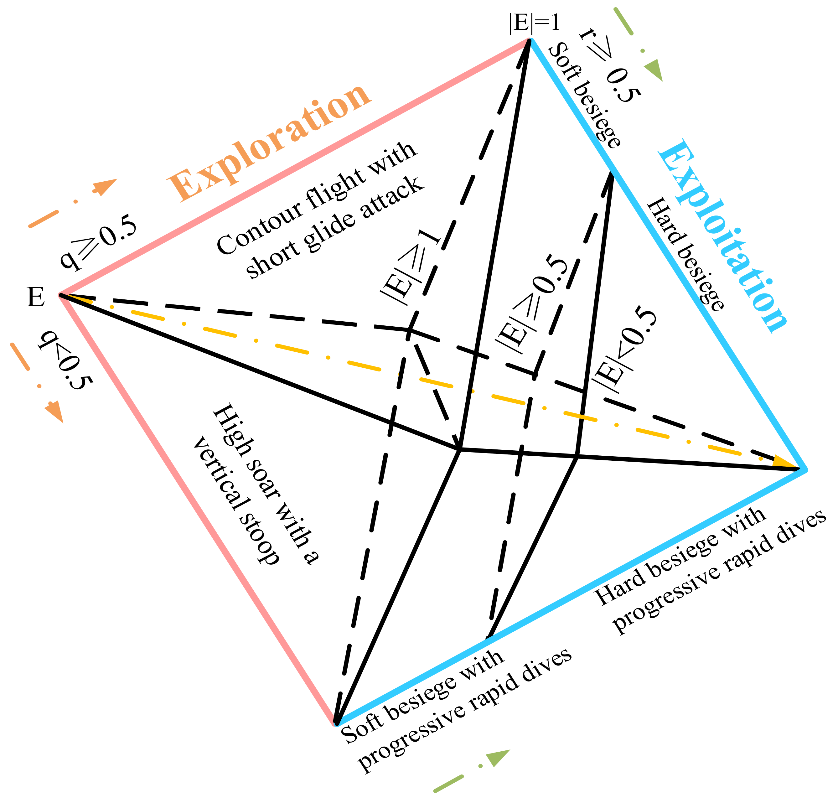
2.2. Harris’s Hawks Optimizer (HHO)

HHO is a new meta-heuristic optimization algorithm proposed by Heidari et al. in 2019. It is inspired by the unique cooperative foraging activities of Harris’s hawk. Harris’s hawk can show a variety of chasing patterns according to the dynamic nature of the environment and the escaping patterns of the prey. These switching activities are conducive to confuse the running prey, and these cooperative strategies can help Harris’s hawk chase the detected prey to exhaustion, which increases its vulnerability. The brief description of mathematical model is as follows.

2.2.1. Exploration Phase

The Harris’s hawks usually perch on some random locations, wait, and monitor the desert to detect the prey. There are two perching strategies based on the positions of other family members and the prey or random tall trees, which is selected in accordance with the random q value.
X ( t + 1 ) = X r ( t ) r 1 | X r ( t ) 2 r 2 X ( t ) | q 0.5 ( X p r e y ( t ) X m ( t ) ) r 3 ( L B + r 4 ( U B L B ) ) q < 0.5
X m ( t ) = 1 N i = 1 N X i ( t )
where X r ( t ) is the position of a random hawk, X p r e y ( t ) represents the position of the prey, that is the best position obtained so far, and X m ( t ) denotes the average position of the current population. N is total number of hawks, U B and L B are the upper and lower bound of the problem, and q , r 1 , r 2 , r 3 , and r 4 are random numbers between 0 and 1.

2.2.2. Transition from Exploration to Exploitation Phase

The HHO algorithm has a transition mechanism from exploration to exploitation phase based on the escaping energy of the prey and then changes the different exploitative behaviors. The energy of the prey is modelled as follows, which decreases during the escaping behaviour.
E = 2 E 0 ( 1 t T )
where E represents the escaping energy of the prey, E 0 is the initial state of the energy, and t and T are the current and maximum number of iterations, respectively. When | E | 1 , the algorithm performs the exploration stage, and when | E | < 1 , the algorithm performs the exploitation phase.

2.2.3. Exploitation Phase

In this phase, four different chasing and attacking strategies are proposed on the basis of the escaping energy of the prey and chasing styles of the Harris’s hawks. Except for the escaping energy, parameter r is also utilized to choose the chasing strategy, which indicates the chance of the prey in successfully escaping ( r < 0.5 ) or not ( r 0.5 ) before attack.
  • Soft besiege
When r 0.5 and | E | 0.5 , the prey still has enough energy and tries to escape, so the Harris’s hawks encircle it softly to make the prey more exhausted and then attack it. This behaviour is modeled as follows:
X ( t + 1 ) = Δ X ( t ) E | J X p r e y ( t ) X ( t ) |
Δ X ( t ) = X p r e y ( t ) X ( t )
J = 2 ( 1 r 5 )
where Δ X ( t ) indicates the difference between the position of the prey and the current position, J represents the random jump strength of the prey, X p r e y ( t ) represents the position of the prey, X ( t ) is the current position, and r 5 is a random number within (0, 1).
  • Hard besiege
When r 0.5 and | E | < 0.5 , the prey has a low escaping energy, and the Harris’s hawks encircle the prey readily and finally attack it. In this situation, the positions are updated as follows:
X ( t + 1 ) = X p r e y ( t ) E | Δ X ( t ) |
  • Soft besiege with progressive rapid dives
When | E | 0.5 and r < 0.5 , the prey has enough energy to successfully escape, so the Harris’s hawks perform soft besiege with several rapid dives around the prey and try to progressively correct its position and direction. This behaviour is modeled as follows:
Y = X p r e y ( t ) E | J X p r e y ( t ) X ( t ) |
Z = Y + S × L F ( D )
L F ( x ) = 0.01 × u × σ | υ | 1 β
σ = Γ ( 1 + β ) × s i n ( π β 2 ) Γ ( 1 + β 2 ) × β × 2 ( β 1 2 ) 1 β
X ( t + 1 ) = Y i f   F ( Y ) < F ( X ( t ) ) Z i f   F ( Z ) < F ( X ( t ) )
where D is the dimension size of the problem, and S is a random vector. L F is Levy flight function, which is utilized to mimic the deceptive motions of the prey. u and v are random values between 0 and 1, and β is a constant number equal to 1.5. Note that only the better position between Y and Z is selected as the next position.
  • Hard besiege with progressive rapid dives
When | E | < 0.5 and r < 0.5 , the prey does not have enough energy to escape, so the hawks perform a hard besiege to decrease the distance between their average position and the prey and finally attack and kill the prey. The mathematical representation of this behaviour is as follows:
Y = X p r e y ( t ) E | J X p r e y ( t ) X m ( t ) |
Z = Y + S × L F ( D )
X ( t + 1 ) = Y i f   F ( Y ) < F ( X ( t ) ) Z i f   F ( Z ) < F ( X ( t ) )
Note that only the better position between Y and Z will be the next position for the new iteration.

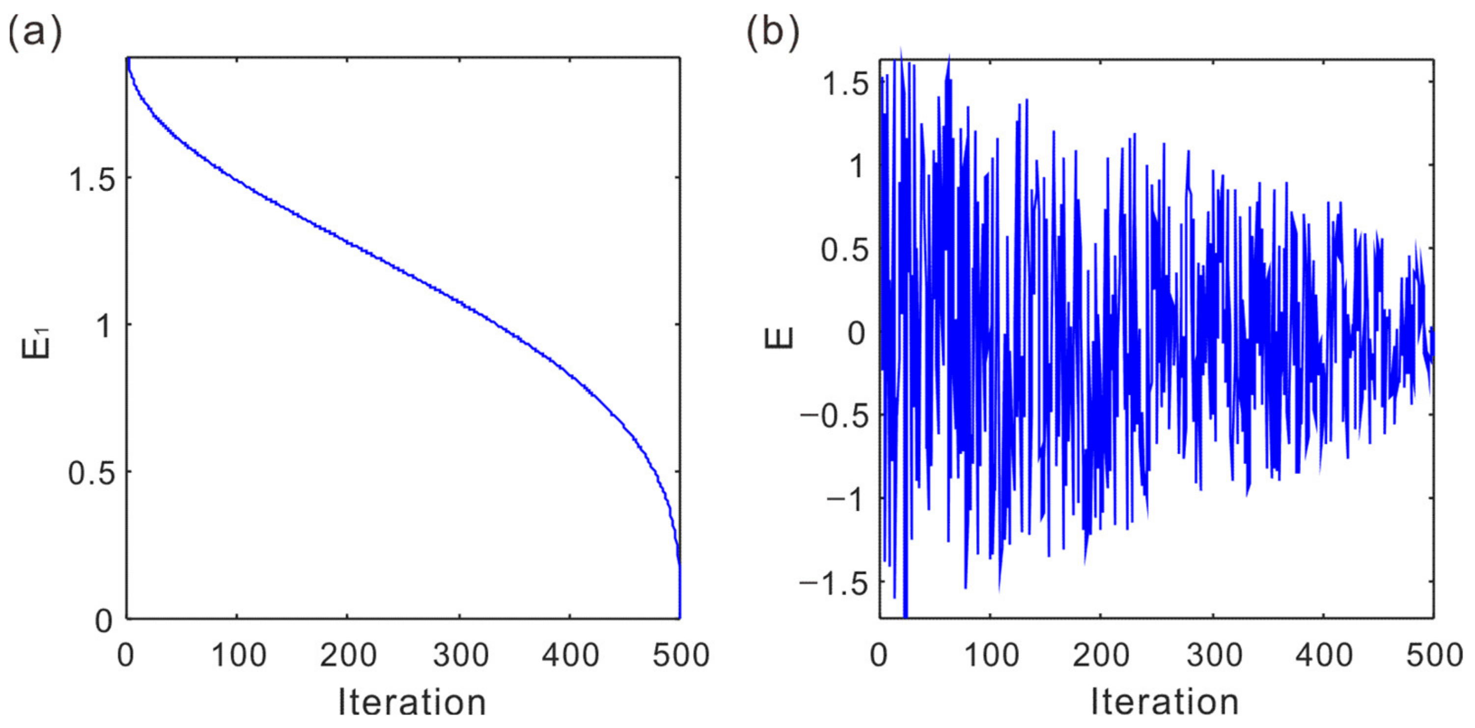
2.3. Nonlinear Escaping Energy Parameter

In the original HHO algorithm, the escaping energy E is used to control the transition from exploration to exploitation phase. The parameter E is linearly reduced from 2 to 0, that is, only local search is performed in the second half of the iterations, which is easy to fall into local optima. In order to overcome this shortcoming of the algorithm, another way to update the escaping energy E is utilized [56]:
E = E 1 ( 2 × rand - 1 )
E 1 = 2 × ( 1 - t T 1 / 3 ) 1 / 3
where t and T are the current and maximum number of iterations, respectively. It can be seen from Figure 2a that E 1 decreases rapidly in the early stage of the iterations, which controls the global search ability of the algorithm and changes slowly in the middle of the iterations. E 1 also balances the global and local search capabilities and decreases rapidly in the later stage of the iterations to speed up the local search. E can perform global search and local search in the whole iterative process. It mainly performs global search in the early stage and retains the possibility of global search while mainly performing local search in the later stage, as shown in Figure 2b.

2.4. Random Opposition-Based Learning (ROBL)

Opposition-based learning (OBL) is a powerful optimization tool proposed by Tizhoosh [57]. The main idea of OBL is simultaneously considering the fitness of an estimate and its corresponding opposite estimate to obtain a better candidate solution. The OBL concept has successfully been used in varieties of meta-heuristics algorithms [58,59,60,61,62] to improve the convergence speed. Different from the original OBL, this paper utilizes an improved OBL strategy, called random opposition-based learning (ROBL) [63], which is defined by:
x ^ j = l j + u j r a n d × x j , j = 1 , 2 , , n
where x ^ j represents the opposite solution, l j and u j are the lower and upper bound of the problem in jth dimension, and rand is a random number within (0, 1). The opposite solution described by Equation (26) is more random than the original OBL and can effectively help the population jump out of the local optima.

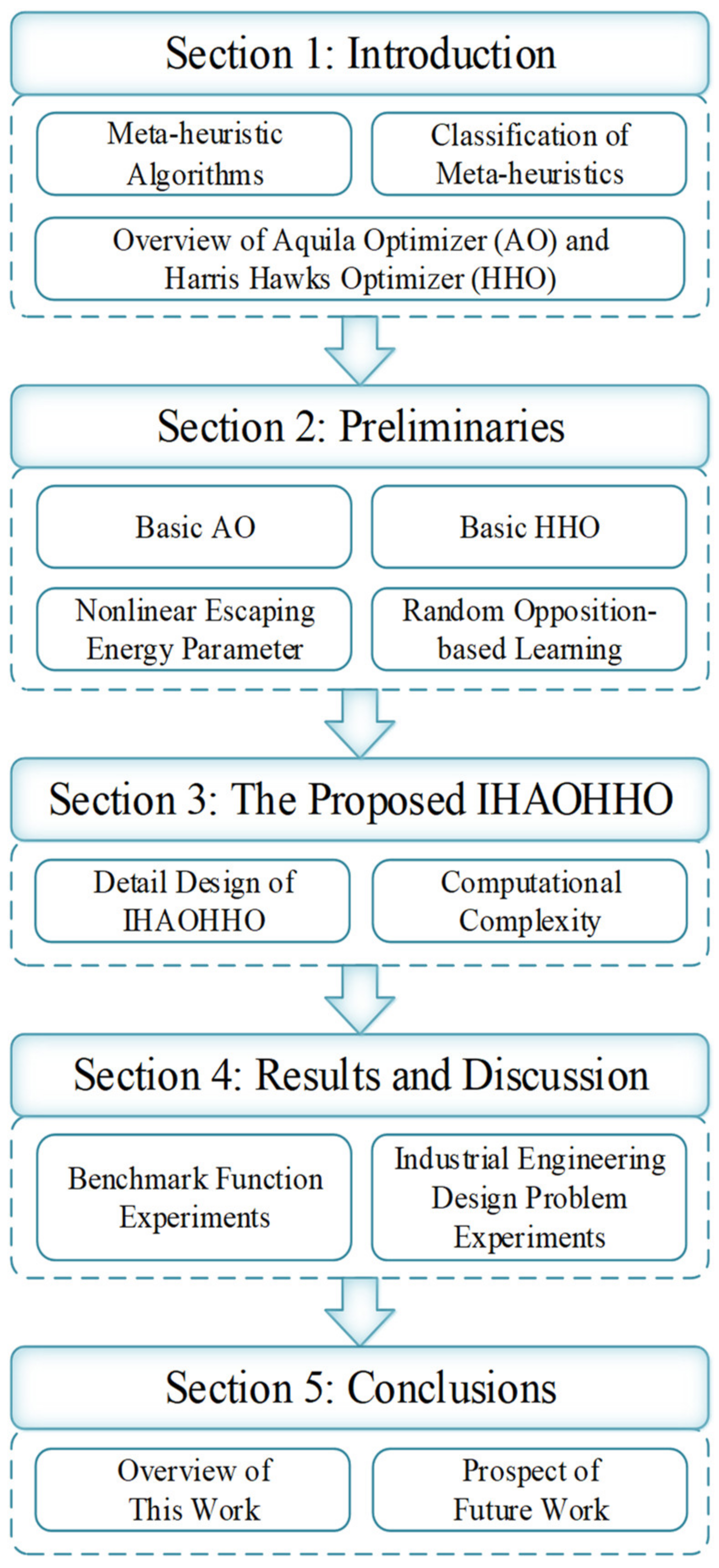
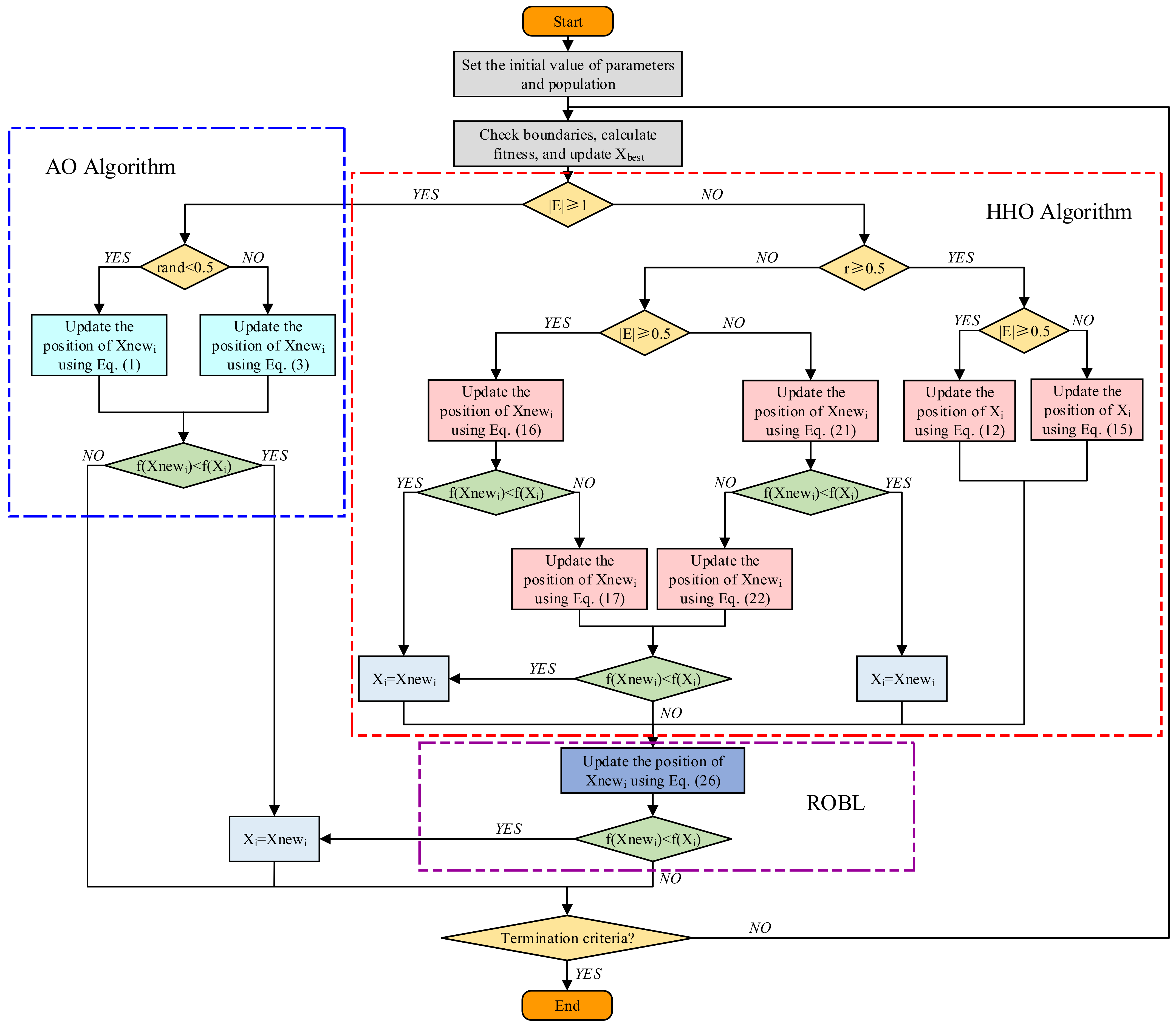
3. The Proposed IHAOHHO Algorithm

3.1. The Detail Design of IHAOHHO

The exploration phase of AO mimics the hunting behaviour for fast-moving prey with a wide flying area, making AO have a strong global search ability and fast convergence speed. However, the selected search space is not exhaustively searched during the exploitation phase. The effect of Levy flight is relatively weak, leading to premature convergence. In a word, the AO algorithm possesses strong randomness and fast convergence speed in the global exploration phase. However, it is easy to fall into local optima in the local exploitation stage. For the HHO algorithm, the transition from global to local search is realized based on the energy attenuation of the prey. In the early iterations, which reflect the exploration phase, the diversity of the population is insufficient, and the convergence speed is slow. As the number of iterations increases, the energy of prey decreases, and the algorithm enters the stage of local exploitation. Four different hunting strategies are adopted in the light of the energy and escape probability of the prey. The Levy flight term is added in the exploitation phase. Whether to use Levy flight to update positions is decided by fitness values so that the algorithm can jump out of the local optima to a certain extent.
Therefore, we combine the global exploration phase of AO and the local exploitation phase of HHO to give full play to the advantages of these two algorithms. The global search capability, faster convergence speed, and the ability to jump out of the local optima of the algorithm are all retained. Meanwhile, a nonlinear escaping energy mechanism is utilized to control the transition from exploration to exploitation phase, which retains the possibility of global search in the later iterations. ROBL strategy is added to the exploitation phase to enhance further the ability to jump out of the local optima. All these strategies improve the convergence speed and accuracy of the hybrid algorithm and effectively enhance the overall optimization performance of the algorithm. This improved hybrid Aquila Optimizer and Harris Hawks Optimization algorithm is named IHAOHHO. Different phases of IHAOHHO are shown in Figure 3. The pseudo-code of IHAOHHO is given in Algorithm 1, and the summarized flowchart is illustrated in Figure 4.
Algorithm 1 Pseudo-code of IHAOHHO.
1: Set initial values of the population size N and the maximum number of iterations T
2: Initialize positions of the population X
3: While t < T
4:  For i = 1 to N
5:   Check if the position goes out of the search space boundary, and bring it back.
6:   Calculate the fitness of Xi
7:   Update Xbest
8:  End for
9:  Update x, y, QF, G1, G2, E1
10:   For i = 1 to N
11:   Update E using Equation (24)  % Nonlinear escaping energy parameter
12:   If |E| ≥ 1          % Exploration part of AO
13:    If rand < 0.5
14:     Update the position of Xnewi using Equation (1)
15:      If f(Xnewi) < f(Xi)
16:       Xi = Xnewi
17:      End if
18:     Else
19:     Update the position of Xnewi using Equation (3)
20:      If f(Xnewi) < f(Xi)
21:       Xi = Xnewi
22:      End if
23:    End if
24:   Else         % Exploitation part of HHO
25:    If r ≥ 0.5 and |E| ≥ 0.5
26:     Update the position of Xi using Equation (12)
27:    End if
28:    If r ≥ 0.5 and |E| < 0.5
29:     Update the position of Xi using Equation (15)
30:    End if
31:    If r < 0.5 and |E| ≥ 0.5
32:     Update the position of Xnewi using Equation (16)
33:     If f(Xnewi) < f(Xi)
34:      Xi = Xnewi
35:     Else
36:      Update the position of Xnewi using Equation (17)
37:      If f(Xnewi) < f(Xi)
38:       Xi = Xnewi
39:      End if
40:     End if
41:    End if
42:    If r < 0.5 and |E| < 0.5
43:     Update the position of Xnewi using Equation (21)
44:     If f(Xnewi) < f(Xi)
45:      Xi = Xnewi
46:     Else
47:      Update the position of Xnewi using Equation (22)
48:      If f(Xnewi) < f(Xi)
49:       Xi = Xnewi
50:      End if
51:     End if
52:    End if
53:    Update the position of Xnewi using Equation (26)  % ROBL
54:    If f(Xnewi) < f(Xi)
55:     Xi = Xnewi
56:    End if
57:   End if
58:   t = t + 1
59: End for
60:  End while
61:  Return Xbest

3.2. Computational Complexity of IHAOHHO

Computation complexity is a key metric for an algorithm to evaluate its time consumption during operation. The computational complexity of the IHAOHHO algorithm depends on three processes: initialization, evaluation of fitness, and updating of hawks. In the initialization stage, the computational complexity of positions generated of N hawks is O(N × D), where D is dimension size of the problem. Then, the computational complexity of fitness evaluation for the best solution is O(N) during the iteration process. Considering the worst condition, the computational complexities of position updating of hawks and fitness comparison are O(3 × N × D) and O(3 × N), respectively. In a word, the total computational complexity of the proposed IHAOHHO algorithm is O(N × D + (3 × D + 4) × N × T).

4. Results and Discussion

In this section, two main experiments were carried out to evaluate the performance of the IHAOHHO algorithm. The first kind of experiments is benchmark function experiments, which aimed to evaluate the performance of IHAOHHO in solving 23 numerical optimization problems. The second experiment is industrial engineering design problems, which aimed to evaluate the performance of IHAOHHO in solving real-world problems. All experiments are implemented in MATLAB R2016a on a PC with Intel (R) core (TM) i5-9500 CPU @ 3.00 GHz and RAM 2 GB memory on OS windows 10.

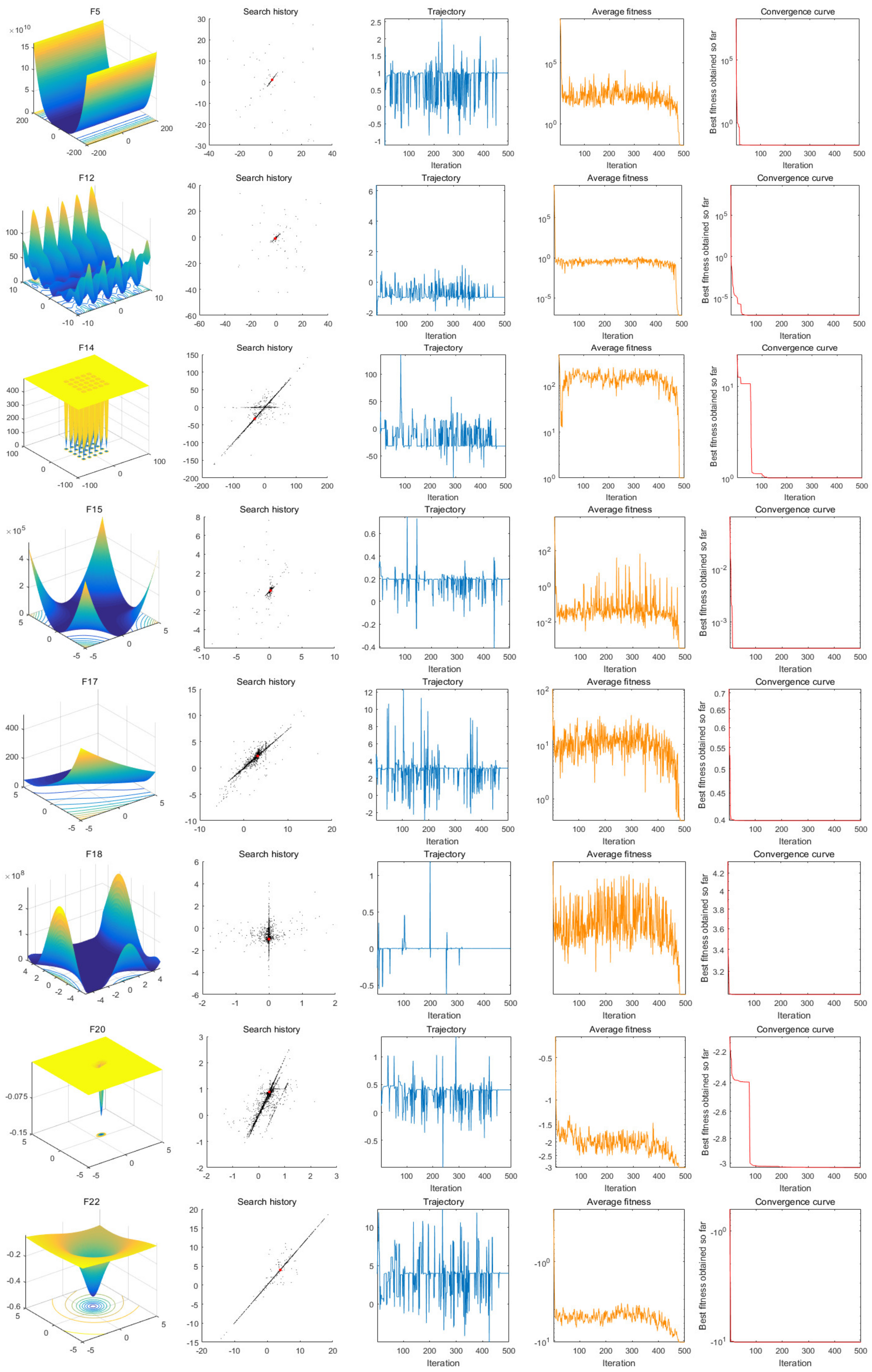
4.1. Benchmark Function Experiments

To investigate the performance of the IHAOHHO algorithm, 23 standard benchmark functions of three different types were utilized for testing [64]. The main characteristic of the first type, namely unimodal benchmark functions, is that there is only one global optimum with no local optima. These test functions can be used to evaluate the exploitation capability and convergence rate of an algorithm. The second type, namely multimodal benchmark functions, has a global optimum and multiple local optima, which includes general and fixed-dimension multimodal test functions. This type of functions was utilized to evaluate the exploitation and local optima avoidance capability of the algorithm. The benchmark function details, including dimensions, ranges, and optima, are listed in Table 1, Table 2 and Table 3.
For verification of the results, the IHAOHHO algorithm was compared with the original AO and HHO; SMA as one of the recent algorithms; SSA, WOA, and GWO as several classical meta-heuristic algorithms; and PSO as the most well-known swarm intelligence algorithm. For all these algorithms, we set the population size N = 30, dimension size D = 30, maximum number of iterations T = 500, and ran them 30 times independently. The parameter settings of each algorithm are shown in Table 4. After all, the average and standard deviation results of these test functions are exhibited in Table 4, Table 5 and Table 6. Figure 5 shows the convergence curves of 23 test functions. The partial search history, trajectory and average fitness maps are represented in Figure 6. Wilcoxon signed-rank test results are also listed in Table 6. The detailed data analysis is given in the following subsections.

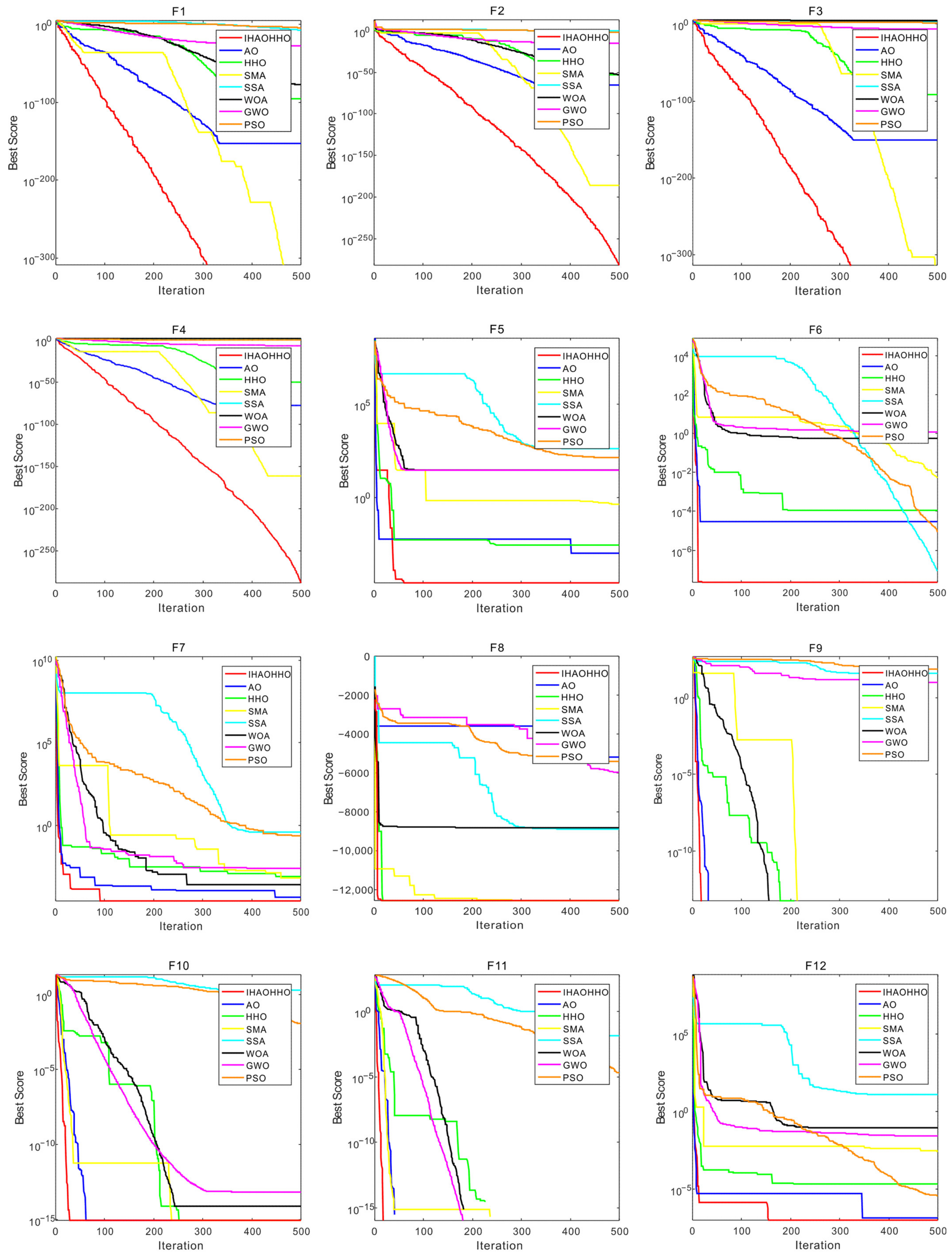
4.1.1. Evaluation of Exploitation Capability (Functions F1–F7)

Functions F1–F7 are used to investigate the exploitation capability of the algorithm since they have only one global optimum and no local optima. It can be seen from Table 5 that IHAOHHO can achieve much better results than other meta-heuristic algorithms excluding F6. For F1 and F3, IHAOHHO can find the theoretical optimum. For all unimodal functions excluding F6, IHAOHHO gets the smallest average values and standard deviations compared to other algorithms, which indicate the best accuracy and stability. Hence, the exploitation capability of the proposed IHAOHHO algorithm is excellent.

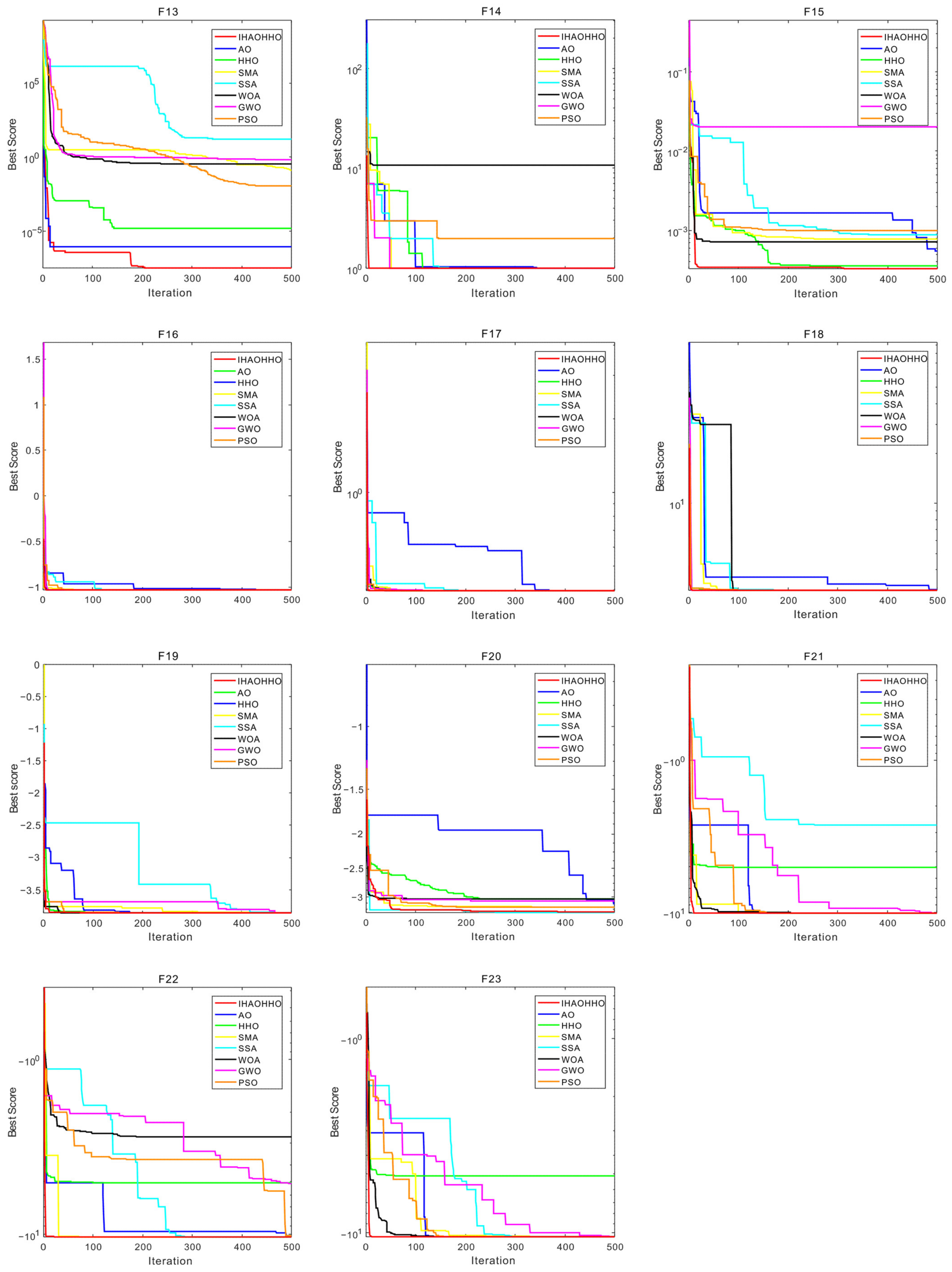
4.1.2. Evaluation of Exploration Capability (Functions F8–F23)

Multimodal functions F8–F23 contain plentiful local optima whose number increases exponentially with the dimension size of the problem. This kind of functions is very useful to evaluate the exploration ability of the algorithm. From the results shown in Table 5, IHAOHHO outperforms other algorithms in most of the multimodal and fixed-dimension multimodal functions. For multimodal functions F8–F13, IHAOHHO almost obtains all the best average values and standard deviations. Among ten fixed-dimensions multimodal functions F14–F23, IHAOHHO achieves the best accuracy of eight functions and best stability of four functions. These results indicate that IHAOHHO also provides robust exploitation capability.

4.1.3. Analysis of Convergence Behavior

In the light of the mathematical formula of the IHAOHHO algorithm, search agents tend to investigate promising regions of the search space widely and then exploit it in detail. Search agents change drastically in early iterations and then converge gradually as the number of iterations increases. Convergence curves of the proposed IHAOHHO and AO, HHO, SMA, SSA, WOA, GWO, and PSO for 23 benchmark functions are provided in Figure 5, which shows the convergence rate of algorithms. It can be seen that IHAOHHO shows great superiority compared to other state-of-the-art algorithms. The IHAOHHO algorithm presents three different convergence behaviors during optimization processes. Firstly, for F1-F4, IHAOHHO gradually converges to the optimal values at a faster speed than other algorithms, and the optimal value is better than the others in three of the functions. The second behaviour is extremely fast convergence speed, as observed in F6, F8–F11, F14–F19, and F21–F23. For these functions, IHAOHHO can find the optimum at an extremely fast speed within 20 iterations, and the accurate approximation of the global optimum is almost the best. The last behaviour is observed in F5, F7, F12, F13, and F20 and shows the local optimum avoidance capability of IHAOHHO. The proposed algorithm jumps out of the local optimum after several times of stagnation. This is probably due to the effect of nonlinear escaping energy parameter. Overall, IHAOHHO can efficiently achieve great solutions for all these 23 standard benchmark functions.
In addition, the search history, trajectory, and average fitness figures of several functions are given in Figure 6. Search history figures show us how the algorithm explores and exploits the search space while solving optimization problems. Trajectory figures reveal the order in which an algorithm explores and exploits the search space. Meanwhile, average fitness presents if exploration and exploitation are conducive to improve the first random population, and an accurate approximation of the global optimum can be found in the end. Inspecting Figure 6, the IHAOHHO algorithm samples the most promising areas observed from search histories. Because of the fast convergence, the vast majority of search agents are concentrated near the global optimum. From trajectory and average fitness maps, it can be noticed that exploration almost spread throughout the iterative process until the last 50 iterations focused on exploitation, and average fitness decreased abruptly and leveled off accordingly. The average fitness figures also show the great improvement of the first random population and the acquisition of the final global optimal accurate approximation.

4.1.4. The Wilcoxon Test

Furthermore, the Wilcoxon signed-rank test results are listed in Table 6, which is used to evaluate the statistical performance differences between the proposed IHAOHHO algorithm with other algorithms. It is worth noting that a p-value less than 0.05 means that there is a significant difference between the two compared algorithms. In the light of this criterion, IHAOHHO outperforms all other algorithms in varying degrees. This superiority is statistically significant on unimodal functions F1–F7, which indicates that IHAOHHO benefits from high exploitation. IHAOHHO also shows better results on multimodal function F8–F23, from which we may conclude that IHAOHHO has a high capability of exploration to investigate the most promising regions in the search space. To sum up, the IHAOHHO algorithm can provide better results on almost all benchmark functions than other comparative algorithms.

4.1.5. Computation Time

The computation time is useful to assess the efficiency for an algorithm in solving optimization problems. From the computation time results of all algorithms shown in Table 7, it is obvious that IHAOHHO spent more time in solving these benchmark functions than other comparative algorithms, especially the earlier classic methods of SSA, WOA, GWO, and PSO. The computation time of IHAOHHO is also slightly longer than the basic AO and HHO, which may be ascribed to the ROBL strategy. ROBL produces one more candidate solution in each iteration, increasing the computation time. However, the IHAOHHO took less time than SMA on most test functions. In view of the best search performance of IHAOHHO and the rapid development of the computational machines, it is acceptable for the proposed algorithm to improve the optimization performance.

4.2. Experiments on Industrial Engineering Design Problems

Most optimization problems have constraints in the real world, so considering equality and inequality constraints during optimization is a necessary process. In this subsection, four well-known constrained industrial engineering design problems, which include pressure vessel design problem, speed reducer design problem, tension/compression spring design problem, and three-bar truss design problem, were solved to further verify the performance of the proposed IHAOHHO algorithm. The results of IHAOHHO were compared to various classical optimizers proposed in previous studies. The parameter settings were as same as the previous experiments.

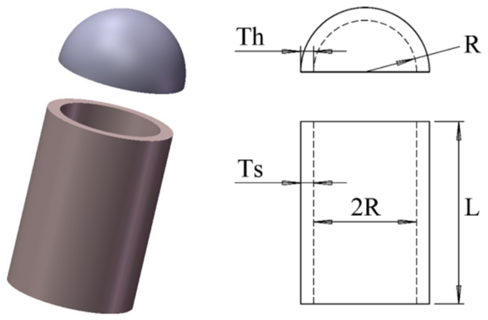
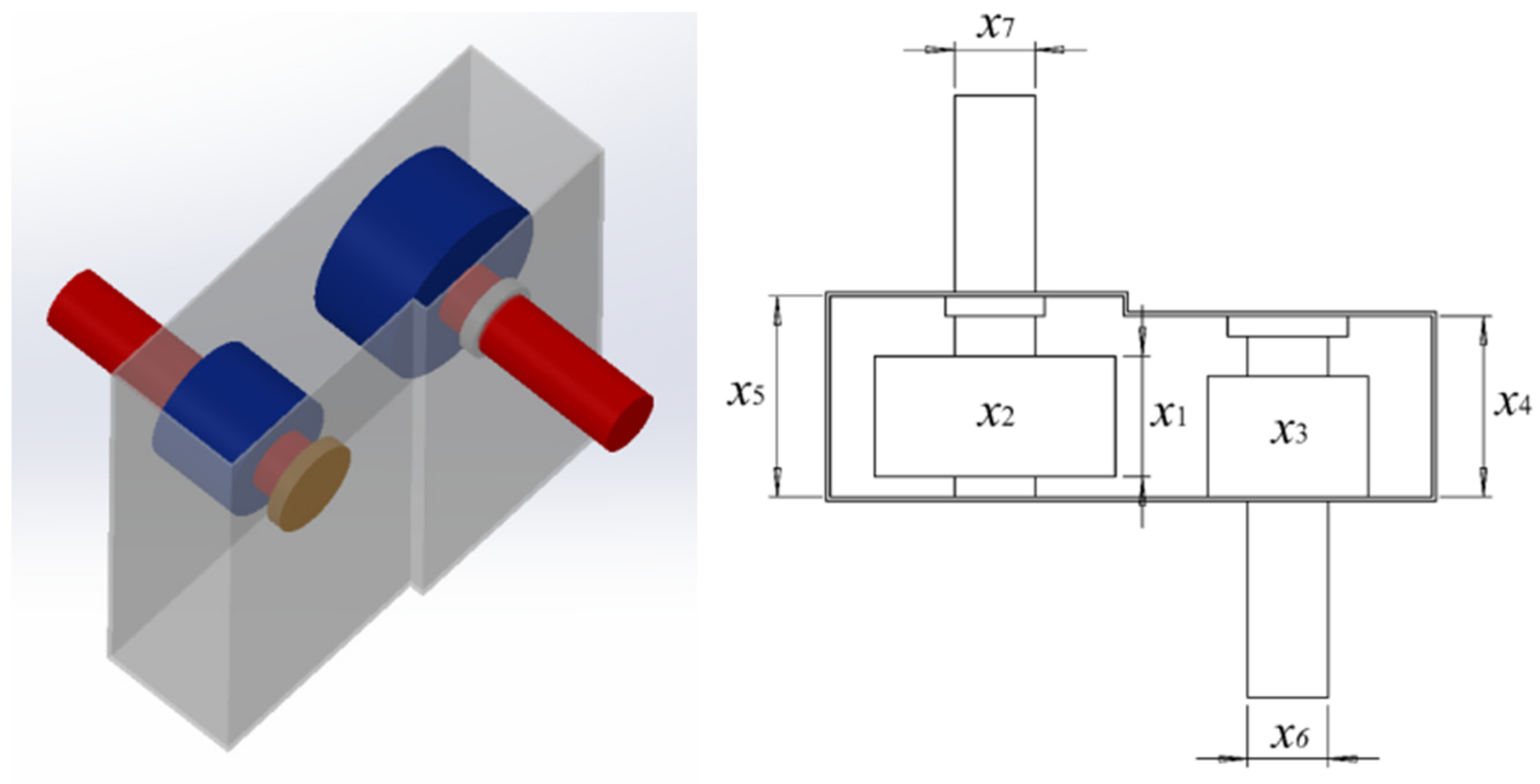
4.2.1. Pressure Vessel Design Problem

The objective of this problem was to minimize the fabrication cost of the cylindrical pressure vessel to meet the pressure requirements. As shown in Figure 7, four structural parameters in this problem needed to be minimized, including the thickness of the shell (Ts), the thickness of the head (Th), inner radius (R), and the length of the cylindrical section without the head (L). The formulation of four optimization constraints can be described as follows:
Consider
x = [ x 1   x 2   x 3   x 4 ] = [ T s   T h   R   L ] ,
Minimize
f ( x ) = 0.6224 x 1 x 3 x 4 + 1.7781 x 2 x 3 2 + 3.1661 x 1 2 x 4 + 19.84 x 1 2 x 3 ,
Subject to
g 1 ( x ) = x 1 + 0.0193 x 3 0 , g 2 ( x ) = x 3 + 0.00954 x 3 0 , g 3 ( x ) = π x 3 2 x 4 4 3 π x 3 3 + 1296000 0 , g 4 ( x ) = x 4 240 0 ,
Variable range
0 x 1 99 , 0 x 2 99 , 10 x 3 200 , 10 x 4 200 ,
From the results in Table 8, it is obvious that IHAOHHO can obtain superior optimal values compared to AO, HHO, SMA, WOA, GWO, MVO, GA, ES, and CPSO [65].

4.2.2. Speed Reducer Design Problem

This problem aims to optimize seven variables to minimize the speed reducer’s total weights, which include the face width (x1), module of teeth (x2), a discrete design variable on behalf of the teeth in the pinion (x3), length of the first shaft between bearings (x4), length of the second shaft between bearings (x5), diameters of the first shaft (x6), and diameters of the second shaft (x7). Four constraints—covering stress, bending stress of the gear teeth, stresses in the shafts, and transverse deflections of the shafts, as shown in Figure 8—should be satisfied. The mathematical formulation is represented as follows:
Minimize
f ( x ) = 0.7854 x 1 x 2 2 ( 3.3333 x 3 2 + 14.9334 x 3 43.0934 ) 1.508 x 1 ( x 6 2 + x 7 2 ) + 7.4777 ( x 6 3 + x 7 3 ) ,
Subject to
g 1 ( x ) = 27 x 1 x 2 2 x 3 1 0 , g 2 ( x ) = 397.5 x 1 x 2 2 x 3 2 1 0 , g 3 ( x ) = 1.93 x 4 3 x 2 x 3 x 6 4 1 0 , g 4 ( x ) = 1.93 x 5 3 x 2 x 3 x 7 4 1 0 , g 5 ( x ) = ( 745 x 4 x 2 x 3 ) 2 + 16.9 × 10 6 110.0 x 6 3 1 0 , g 6 ( x ) = ( 745 x 4 x 2 x 3 ) 2 + 157.5 × 10 6 85.0 x 6 3 1 0 , g 7 ( x ) = x 2 x 3 40 1 0 , g 8 ( x ) = 5 x 2 x 1 1 0 , g 9 ( x ) = x 1 12 x 2 1 0 , g 10 ( x ) = 1.5 x 6 + 1.9 x 4 1 0 , g 11 ( x ) = 1.1 x 7 + 1.9 x 5 1 0 ,
Variable range
2.6 x 1 3.6 , 0.7 x 2 0.8 , 17 x 3 28 , 7.3 x 4 8.3 , 7.8 x 5 8.3 , 2.9 x 6 3.9 , 5.0 x 7 5.5 ,
Compared to AO, PSO, AOA, MFO [66], GA, SCA, HS [67], FA [68], and MDA [69], IHAOHHO can obviously achieve better results in the speed reducer design problem, as shown in Table 9.

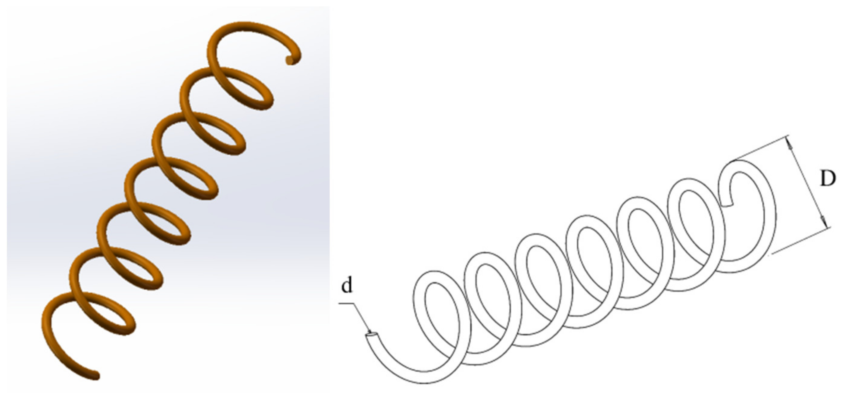
4.2.3. Tension/Compression Spring Design Problem

In this case, the intention is to minimize the weight of the tension/compression spring shown in Figure 9. Constraints on surge frequency, shear stress, and deflection must be satisfied during optimum design. There are three parameters that needed to be minimized, including the wire diameter (d), mean coil diameter (D), and the number of active coils (N). The mathematical form of this problem can be written as follows:
Consider
x = [ x 1   x 2   x 3   x 4 ] = [ d   D   N ] ,
Minimize
f ( x ) = ( x 3 + 2 ) x 2 x 1 2 ,
Subject to
g 1 ( x ) = 1 x 2 3 x 3 71,785 x 1 4 0 , g 2 ( x ) = 4 x 2 2 x 1 x 2 12,566 ( x 2 x 1 3 x 1 4 ) + 1 5108 x 1 2 0 , g 3 ( x ) = 1 140.45 x 1 x 2 2 x 3 0 , g 4 ( x ) = x 1 + x 2 1.5 1 0 ,
Variable range
0.05 x 1 2.00 , 0.25 x 2 1.30 , 2.00 x 3 15.00 ,
The proposed IHAOHHO is compared with AO, HHO, SSA, WOA, GWO, PSO, MVO, GA, and HS algorithms. Results are listed in Table 10 and show that the IHAOHHO can attain the best weight values compared to all other algorithms. Additionally, it is clear that the proposed method found a more accurate design with new parameter values.

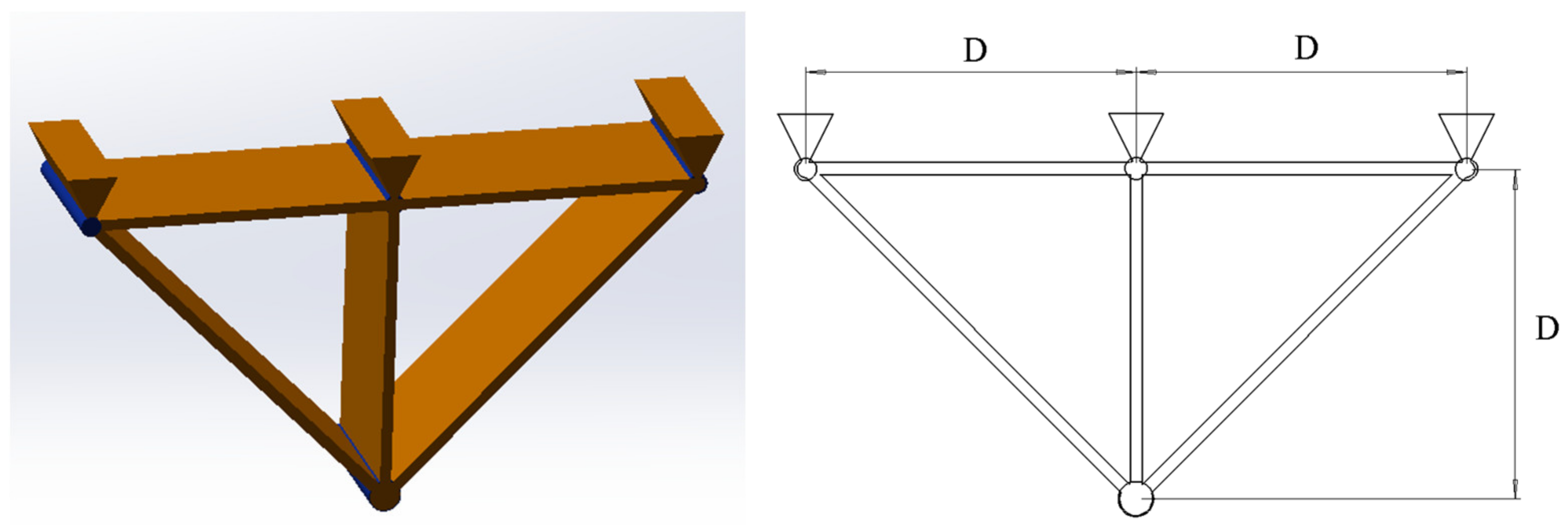
4.2.4. Three-Bar Truss Design Problem

The three-bar truss design problem is a classical optimization application in civil engineering field. The main intention of this case is to minimize the weight of a truss with three bars by considering two structural parameters as illustrated in Figure 10. Deflection, stress, and buckling are the three main constrains. The mathematical formulation of this problem is given:
Consider
x = [ x 1   x 2 ] = [ A 1   A 2 ] ,
Minimize
f ( x ) = ( 2 2 x 1 + x 2 ) l ,
Subject to
g 1 ( x ) = 2 x 1 + x 2 2 x 1 2 + 2 x 1 x 2 P σ 0 , g 2 ( x ) = x 2 2 x 1 2 + 2 x 1 x 2 P σ 0 , g 3 ( x ) = 1 2 x 2 + x 1 P σ 0 ,
Variable range
0 x 1 , x 2 1 ,
where l = 100 cm , P = 2 KN / cm 2 , σ = 2 KN / cm 2 . Results of IHAOHHO for solving three-bar truss design problem are listed in Table 11, which are compared with AO, HHO, SSA, AOA, MVO, MFO, and GOA [70]. It can be observed that IHAOHHO outperforms other optimization algorithms published in the literature.
As a summary, this section demonstrates the superiority of the proposed IHAOHHO algorithms in different characteristics and real case studies. IHAOHHO is able to outperform the original AO and HHO and other well-known algorithms with very competitive results, which were derived from the robust exploration and exploitation capabilities of IHAOHHO. Excellent performance in solving industrial engineering design problems indicates that IHAOHHO can be widely used in real-world optimization problems.

5. Conclusions

This study proposed an improved hybrid Aquila Optimizer and Harris Hawks Optimization by combining the exploration part of AO with the exploitation part of HHO and a nonlinear escaping energy parameter and random opposition-based learning (ROBL) strategy. The proposed method integrated the mentioned search methods to tackle the weakness of the traditional search methods. The proposed IHAOHHO algorithm was tested using 23 mathematical benchmark functions to analyze its exploration, exploitation, local optima avoidance capabilities, and convergence behaviors. Results show competitive results compared to other state-of-the-art meta-heuristic algorithms. To further verify the superiority of IHAOHHO, four industrial engineering design problems were solved. The results are also competitive with other meta-heuristic algorithms.
As future perspectives, binary and multi-objective versions of IHAOHHO will be considered. More applications of this algorithm in different fields are valuable works, including text clustering, scheduling problems, appliances management, parameters estimation, multi-objective engineering problems, feature selection, test classification, image segmentation problems, network applications, sentiment analysis, etc.

Author Contributions

Conceptualization, H.J. and L.A.; methodology, S.W.; software, R.Z.; validation, S.W., Q.L. and R.Z.; formal analysis, S.W.; writing—original draft preparation, S.W.; writing—review and editing, S.W.; visualization, Q.L.; supervision, L.A.; project administration, H.J.; funding acquisition, S.W. and H.J. All authors have read and agreed to the published version of the manuscript.

Funding

This research was funded by the Sanming University Introduces High-level Talents to Start Scientific Research Funding Support Project, grant number 20YG01, 20YG14; the Guiding Science and Technology Projects in Sanming City, grant number 2020-S-39, 2020-G-61, 2021-S-8; the Educational Research Projects of Young and Middle-aged Teachers in Fujian Province, grant number JAT200638, JAT200618; the Scientific Research and Development Fund of Sanming University, grant number B202029, B202009; Collaborative education project of industry university cooperation of the Ministry of Education, grant number 202002064014; School level education and teaching reform project of Sanming University, grant number J2010306, J2010305; and Higher education research project of Sanming University, grant number SHE2102, SHE2013.

Institutional Review Board Statement

Not applicable.

Informed Consent Statement

Not applicable.

Data Availability Statement

Not applicable.

Conflicts of Interest

The authors declare no conflict of interest.

References

  1. Abualigah, L.; Diabat, A. Advances in sine cosine algorithm: A comprehensive survey. Artif. Intell. Rev. 2021, 54, 2567–2608. [Google Scholar] [CrossRef]
  2. Abualigah, L.; Diabat, A. A comprehensive survey of the Grasshopper optimization algorithm: Results, variants, and applications. Neural Comput. Appl. 2020, 32, 15533–15556. [Google Scholar] [CrossRef]
  3. Holland, J.H. Genetic algorithms. Sci. Am. 1992, 267, 66–72. [Google Scholar] [CrossRef]
  4. Storn, R.; Price, K. Differential evolution-a simple and efficient heuristic for global optimization over continuous spaces. J. Glob. Optim. 1997, 11, 341–359. [Google Scholar] [CrossRef]
  5. Koza, J.R. Genetic Programming: On the Programming of Computers by Means of Natural Selection; MIT Press: Cambridge, MA, USA, 1992. [Google Scholar]
  6. Rechenberg, I. Evolutionsstrategien. In Simulationsmethoden in der Medizin und Biologie; Springer: Berlin/Heidelberg, Germany, 1978; Volume 8, pp. 83–114. [Google Scholar]
  7. Simon, D. Biogeography-based optimization. IEEE Trans. Evol. Comput. 2008, 12, 702–713. [Google Scholar] [CrossRef] [Green Version]
  8. Yao, X.; Liu, Y.; Lin, G. Evolutionary programming made faster. IEEE Trans. Evol. Comput. 1999, 3, 82–102. [Google Scholar] [CrossRef] [Green Version]
  9. Dasgupta, D.; Michalewicz, Z. Evolutionary Algorithms in Engineering Applications; DBLP: Trier, Germany, 1997. [Google Scholar]
  10. Kirkpatrick, S.; Gelatt, C.D.; Vecchi, M.P. Optimization by simmulated annealing. Science 1983, 220, 671–680. [Google Scholar] [CrossRef] [PubMed]
  11. Erol, O.K.; Eksin, I. A new optimization method: Big bang-big crunch. Adv. Eng. Softw. 2006, 37, 106–111. [Google Scholar] [CrossRef]
  12. Rashedi, E.; Nezamabadi-Pour, H.; Saryazdi, S. GSA: A Gravitational Search Algorithm. Inf. Sci. 2009, 179, 2232–2248. [Google Scholar] [CrossRef]
  13. Webster, B.; Bernhard, P.J. A local search optimization algorithm based on natural principles of gravitation. In Information & Knowledge Engineering, Proceedings of the 2003 International Conference on Information and Knowledge Engineering (IKE’03), Las Vegas, NV, USA, 23–26 June 2003; DBLP: Trier, Germany, 2003. [Google Scholar]
  14. Asef, F.; Majidnezhad, V.; Feizi-Derakhshi, M.R.; Parsa, S. Heat transfer relation-based optimization algorithm (HTOA). Soft Comput. 2021, 1–30. [Google Scholar] [CrossRef]
  15. Kaveh, A.; Talatahari, S. A novel heuristic optimization method: Charged system search. Acta Mech. 2010, 213, 267–289. [Google Scholar] [CrossRef]
  16. Alatas, B. ACROA: Artificial Chemical Reaction Optimization Algorithm for global optimization. Expert Syst. Appl. 2011, 38, 13170–13180. [Google Scholar] [CrossRef]
  17. Formato, R.A. Central force optimization: A new metaheuristic with applications in applied electromagnetics. Prog. Electromag. Res. 2007, 77, 425–491. [Google Scholar] [CrossRef] [Green Version]
  18. Kaveh, A.; Khayatazad, M. A new meta-heuristic method: Ray optimization. Comput. Struct. 2012, 112, 283–294. [Google Scholar] [CrossRef]
  19. Hatamlou, A. Black hole: A new heuristic optimization approach for data clustering. Inf. Sci. 2013, 222, 175–184. [Google Scholar] [CrossRef]
  20. Du, H.; Wu, X.; Zhuang, J. Small-world optimization algorithm for function optimization. In Advances in Natural Computation, Advances in Natural Computation, Second International Conference; ICNC: Xi’an, China, 2006. [Google Scholar]
  21. Shah-Hosseini, H. Principal components analysis by the galaxy-based search algorithm: A novel metaheuristic for continuous optimisation. Int. J. Comput. Sci. Eng. 2011, 6, 132–140. [Google Scholar] [CrossRef]
  22. Moghaddam, F.F.; Moghaddam, R.F.; Cheriet, M. Curved space optimization: A random search based on general relativity theory. arXiv 2012, arXiv:1208.2214. [Google Scholar]
  23. Mirjalili, S.; Mirjalili, S.M.; Hatamlou, A. Multi-Verse Optimizer: A nature-inspired algorithm for global optimization. Neural Comput. Appl. 2015, 27, 495–513. [Google Scholar] [CrossRef]
  24. Mirjalili, S. SCA: A Sine Cosine Algorithm for Solving Optimization Problems. Knowl.-Based Syst. 2016, 96. [Google Scholar] [CrossRef]
  25. Abualigah, L.; Diabat, A.; Mirjalili, S.; Elaziz, M.A.; Gandomi, A.H. The Arithmetic Optimization Algorithm. Comput. Methods Appl. Mech. Eng. 2021, 376, 113609. [Google Scholar] [CrossRef]
  26. Kennedy, J.; Eberhart, R. Particle swarm optimization. In Proceedings of the 1995 IEEE International Conference on Neural Networks (ICNN ’93), Perth, WA, Australia, 27 November–1 December 1995; IEEE: Piscataway, NJ, USA, 1995. [Google Scholar]
  27. Dorigo, M.; Birattari, M.; Stutzle, T. Ant colony optimization. IEEE Comput. Intell. 2006, 1, 28–39. [Google Scholar] [CrossRef]
  28. Mucherino, A.; Seref, O.; Seref, O.; Kundakcioglu, O.E.; Pardalos, P. Monkey search: A novel metaheuristic search for global optimization. Am. Inst. Phys. 2007, 953, 162–173. [Google Scholar] [CrossRef]
  29. Yang, X.S. Firefly algorithm, stochastic test functions and design optimization. Int. J. Bio-Inspired Comput. 2010, 2, 78–84. [Google Scholar] [CrossRef]
  30. Yang, X.S. A new metaheuristic bat-inspired algorithm. In Nature Inspired Cooperative Strategies for Optimization (NICSO); Springer: Berlin/Heidelberg, Germany, 2010. [Google Scholar]
  31. Gandomi, A.H.; Alavi, A.H. Krill Herd: A new bio-inspired optimization algorithm. Commun. Nonlinear Sci. Numer. Simul. 2012, 17, 4831–4845. [Google Scholar] [CrossRef]
  32. Mirjalili, S.; Mirjalili, S.M.; Lewis, A. Grey wolf optimizer. Adv. Eng. Softw. 2014, 69, 46–61. [Google Scholar] [CrossRef] [Green Version]
  33. Gandomi, A.H.; Yang, X.S.; Alavi, A.H. Cuckoo search algorithm: A metaheuristic approach to solve structural optimization problems. Eng. Comput. 2013, 29, 17–35. [Google Scholar] [CrossRef]
  34. Pan, W.T. A new fruit fly optimization algorithm: Taking the financial distress model as an example. Knowl.-Based Syst. 2012, 26, 69–74. [Google Scholar] [CrossRef]
  35. Yang, S.; Jiang, J.; Yan, G. A dolphin partner optimization. In Proceedings of the 2009 WRI Global Congress on Intelligent Systems (GCIS 2009), Xiamen, China, 19–21 May 2009; IEEE: Piscataway, NJ, USA, 2009. [Google Scholar]
  36. Mirjalili, S. The Ant Lion optimizer. Adv. Eng. Softw. 2015, 83, 80–98. [Google Scholar] [CrossRef]
  37. Jia, H.; Peng, X.; Lang, C. Remora optimization algorithm. Expert Syst. Appl. 2021, 185, 115665. [Google Scholar] [CrossRef]
  38. Mirjalili, S.; Lewis, A. The whale optimization algorithm. Adv. Eng. Softw. 2016, 95, 51–67. [Google Scholar] [CrossRef]
  39. Mirjalili, S.; Gandomi, A.H.; Mirjalili, S.Z.; Saremi, S.; Faris, H.; Mirjalili, S.M. Salp swarm algorithm: A bio-inspired optimizer for engineering design problems. Adv. Eng. Softw. 2017, 114, 163–191. [Google Scholar] [CrossRef]
  40. Alsattar, H.A.; Zaidan, A.A.; Zaidan, B.B. Novel meta-heuristic bald eagle search optimisation algorithm. Artif. Intell. Rev. 2020, 53, 2237–2264. [Google Scholar] [CrossRef]
  41. Li, S.M.; Chen, H.L.; Wang, M.J.; Heidari, A.A.; Mirjalili, S. Slime mould algorithm: A new method for stochastic optimization. Future Gener. Comput. Syst. 2020, 111, 300–323. [Google Scholar] [CrossRef]
  42. Heidari, A.A.; Mirjalili, S.; Faris, H.; Aljarah, I.; Mafarja, M.; Chen, H.L. Harris Hawks optimization: Algorithm and applications. Future Gener. Comput. Syst. 2019, 97, 849–872. [Google Scholar] [CrossRef]
  43. Yousri, D.; Fathy, A.; Thanikanti, S.B. Recent methodology based Harris Hawks optimizer for designing load frequency control incorporated in multi-interconnected renewable energy plants. Sustain. Energy Grids Netw. 2020, 22, 100352. [Google Scholar] [CrossRef]
  44. Bui, D.T.; Moayedi, H.; Kalantar, B.; Osouli, A.; Rashid, A. A Novel Swarm Intelligence Technique Harris Hawks Optimization for Spatial Assessment of Landslide Susceptibility. Sensors 2019, 19, 3590. [Google Scholar] [CrossRef] [Green Version]
  45. Golilarz, N.A.; Gao, H.; Demirel, H. Satellite image de-noising with Harris Hawks meta heuristic optimization algorithm and improved adaptive generalized gaussian distribution threshold function. IEEE Access 2019, 7, 57459–57468. [Google Scholar] [CrossRef]
  46. Jia, H.; Peng, X.; Kang, L.; Li, Y.; Sun, K. Pulse coupled neural network based on Harris Hawks optimization algorithm for image segmentation. Multimed Tools Appl. 2020, 79, 28369–28392. [Google Scholar] [CrossRef]
  47. Jia, H.; Lang, C.; Oliva, D.; Song, W.; Peng, X. Dynamic Harris Hawks Optimization with Mutation Mechanism for Satellite Image Segmentation. Remote Sens. 2019, 11, 1421. [Google Scholar] [CrossRef] [Green Version]
  48. Yousri, D.; Mirjalili, S.; Machado, J.A.T.; Thanikantie, S.B.; Elbaksawi, O.; Fathy, A. Efficient fractional-order modified Harris Hawks optimizer for proton exchange membrane fuel cell modeling. Eng. Appl. Artif. Intell. 2021, 100, 104193. [Google Scholar] [CrossRef]
  49. Gupta, S.; Deep, K.; Heidari, A.A.; Moayedi, H.; Wang, M. Opposition-based Learning Harris Hawks Optimization with Advanced Transition Rules: Principles and Analysis. Expert Syst. Appl. 2020, 158, 113510. [Google Scholar] [CrossRef]
  50. Hussien, A.G.; Amin, M. A self-adaptive Harris Hawks optimization algorithm with opposition-based learning and chaotic local search strategy for global optimization and feature selection. Int. J. Mach. Learn. Cyber. 2021, 1–28. [Google Scholar] [CrossRef]
  51. Sihwail, R.; Omar, K.; Ariffin, K.; Tubishat, M. Improved Harris Hawks Optimization Using Elite Opposition-Based Learning and Novel Search Mechanism for Feature Selection. IEEE Access 2020, 8, 121127–121145. [Google Scholar] [CrossRef]
  52. Bao, X.; Jia, H.; Lang, C. A Novel Hybrid Harris Hawks Optimization for Color Image Multilevel Thresholding Segmentation. IEEE Access 2019, 7, 76529–76546. [Google Scholar] [CrossRef]
  53. Houssein, E.H.; Hosney, M.E.; Elhoseny, M.; Oliva, D.; Hassaballah, M. Hybrid Harris Hawks Optimization with Cuckoo Search for Drug Design and Discovery in Chemoinformatics. Sci. Rep. 2020, 10, 14439. [Google Scholar] [CrossRef] [PubMed]
  54. Kaveh, A.; Rahmani, P.; Eslamlou, A.D. An efficient hybrid approach based on Harris Hawks optimization and imperialist competitive algorithm for structural optimization. Eng. Comput. 2021, 4598. [Google Scholar] [CrossRef]
  55. Abualigah, L.; Yousri, D.; Elaziz, M.A.; Ewees, A.A.; Al-qaness, M.A.A.; Gandomi, A.H. Aquila Optimizer: A novel meta-heuristic optimization algorithm. Comput. Ind. Eng. 2021, 157, 107250. [Google Scholar] [CrossRef]
  56. Tang, A.D.; Han, T.; Xu, D.W.; Xie, L. Chaotic Elite Harris Hawk Optimization Algorithm. J. Comput. Appl. 2021, 1–10. Available online: https://kns.cnki.net/kcms/detail/detail.aspx?dbcode=CAPJ&dbname=CAPJLAST&filename=JSJY2021011300H&v=5lc3RO%25mmd2BEUUC%25mmd2FhVq8jnE%25mmd2BxfkAnjCOOEL7xcSF5jPQfItuqOALm2aHD2u1aGLhSpw1 (accessed on 15 January 2021).
  57. Tizhoosh, H. Opposition-based learning: A new scheme for machine intelligence. In Control and Automation, Proceedings of the International Conference on Computational Intelligence for Modeling, Vienna, Austria, 28–30 November 2005; IEEE: Piscataway, NJ, USA, 2005. [Google Scholar]
  58. Rahnamayan, S.; Tizhoosh, H.R.; Salama, M.M.A. Opposition-based differential evolution. IEEE Trans. Evol. Comput. 2014, 12, 64–79. [Google Scholar] [CrossRef] [Green Version]
  59. Jia, Z.; Li, L.; Hui, S. Artificial Bee Colony Using Opposition-Based Learning. Adv. Intell. Syst. Comput. 2015, 329, 3–10. [Google Scholar]
  60. Elaziz, M.A.; Oliva, D.; Xiong, S. An improved Opposition-Based Sine Cosine Algorithm for global optimization. Expert Syst. Appl. 2017, 90, 484–500. [Google Scholar] [CrossRef]
  61. Ewees, A.A.; Elaziz, M.A.; Houssein, E.H. Improved Grasshopper Optimization Algorithm using Opposition-based Learning. Expert Syst. Appl. 2018, 112, 156–172. [Google Scholar] [CrossRef]
  62. Fan, C.; Zheng, N.; Zheng, J.; Xiao, L.; Liu, Y. Kinetic-molecular theory optimization algorithm using opposition-based learning and varying accelerated motion. Soft Comput. 2020, 24, 12709–12730. [Google Scholar] [CrossRef]
  63. Long, W.; Jiao, J.; Liang, X.; Cai, S.; Xu, M. A Random Opposition-Based Learning Grey Wolf Optimizer. IEEE Access 2019, 7, 113810–113825. [Google Scholar] [CrossRef]
  64. Molga, M.; Smutnicki, C. Test Functions for Optimization Needs. 2005. Available online: http://www.robertmarks.org/Classes/ENGR5358/Papers/functions.pdf (accessed on 1 January 2005).
  65. He, Q.; Wang, L. An effective co-evolutionary particle swarm optimization for constrained engineering design problems. Eng. Appl. Artif. Intell. 2007, 20, 89–99. [Google Scholar] [CrossRef]
  66. Mirjalili, S. Moth-flame optimization algorithm: A novel nature-inspired heuristic paradigm. Knowl.-Based Syst. 2015, 89, 228–249. [Google Scholar] [CrossRef]
  67. Geem, Z.W.; Kim, J.H.; Loganathan, G.V. A new heuristic optimization algorithm: Harmony search. Simulation 2001, 76, 60–68. [Google Scholar] [CrossRef]
  68. Baykasoğlu, A.; Ozsoydan, F.B. Adaptive firefly algorithm with chaos for mechanical design optimization problems. Appl. Soft Comput. 2015, 36, 152–164. [Google Scholar] [CrossRef]
  69. Lu, S.; Kim, H.M. A regularized inexact penalty decomposition algorithm for multidisciplinary design optimization problems with complementarity constraints. J. Mech. Des. 2010, 132, 041005. [Google Scholar] [CrossRef] [Green Version]
  70. Saremi, S.; Mirjalili, S.; Lewis, A. Grasshopper optimisation algorithm: Theory and application. Adv. Eng. Softw. 2017, 105, 30–47. [Google Scholar] [CrossRef] [Green Version]
Figure 1. The overview sketch of this paper.
Processes 09 01551 g001
Figure 2. (a) E1 curve and (b) E curve.
Processes 09 01551 g002
Figure 3. Different phases of IHAOHHO.
Processes 09 01551 g003
Figure 4. IHAOHHO algorithm flowchart.
Processes 09 01551 g004
Figure 5. Convergence curves of 23 benchmark functions.
Processes 09 01551 g005aProcesses 09 01551 g005b
Figure 6. Parameter space, search history, trajectory, average fitness, and convergence curve of IHAOHHO.
Processes 09 01551 g006
Figure 7. Pressure vessel design problem.
Processes 09 01551 g007
Figure 8. Speed reducer design problem.
Processes 09 01551 g008
Figure 9. Tension/compression spring design problem.
Processes 09 01551 g009
Figure 10. Three-bar truss design problem.
Processes 09 01551 g010
Table 1. Unimodal benchmark functions.
FunctionDimRangeFmin
F 1 ( x ) = i = 1 n x i 2 30(−100, 100)0
F 2 ( x ) = i = 1 n x i + i = 1 n x i 30(−10, 10)0
F 3 ( x ) = i = 1 n ( j 1 i x j ) 2 30(−100, 100)0
F 4 ( x ) = max i { x i , 1 i n } 30(−100, 100)0
F 5 ( x ) = i = 1 n 1 [ 100 ( x i + 1 x i 2 ) 2 + ( x i 1 ) 2 ] 30(−30,30)0
F 6 ( x ) = i = 1 n ( x i + 5 ) 2 30(−100, 100)0
F 7 ( x ) = i = 1 n i x i 4 + r a n d o m [ 0 , 1 ) 30(−1.28, 1.28)0
Table 2. Multimodal benchmark functions.
FunctionDimRangeFmin
F 8 ( x ) = i = 1 n x i sin ( x i ) 30(−500, 500)−418.9829 × 30
F 9 ( x ) = i = 1 n [ x i 2 10 cos ( 2 π x i ) + 10 ] 30(−5.12, 5.12)0
F 10 ( x ) = 20 exp ( 0.2 1 n i = 1 n x i 2 ) exp ( 1 n i = 1 n cos ( 2 π x i ) ) + 20 + e 30(−32, 32)0
F 11 ( x ) = 1 4000 i = 1 n x i 2 i = 1 n cos ( x i i ) + 1 30(−600, 600)0
F 12 ( x ) = π n { 10 sin ( π y 1 ) + i = 1 n 1 ( y i 1 ) 2 [ 1 + 10 sin 2 ( π y i + 1 ) ] + ( y n 1 ) 2 } + i = 1 n u ( x i , 10 , 100 , 4 ) , where   y i = 1 + x i + 1 4 , u ( x i , a , k , m ) = k ( x i a ) m x i > a 0 a < x i < a k ( x i a ) m x i < a 30(−50, 50)0
F 13 ( x ) = 0.1 ( sin 2 ( 3 π x 1 ) + i = 1 n ( x i 1 ) 2 [ 1 + sin 2 ( 3 π x i + 1 ) ] + ( x n 1 ) 2 [ 1 + sin 2 ( 2 π x n ) ] ) + i = 1 n u ( x i , 5 , 100 , 4 ) 30(−50, 50)0
Table 3. Fixed-dimension multimodal benchmark functions.
FunctionDimRangeFmin
F 14 ( x ) = ( 1 500 + j = 1 25 1 j + i = 1 2 ( x i a i j ) 6 ) 1 2(−65, 65)1
F 15 ( x ) = i = 1 11 [ a i x 1 ( b i 2 + b i x 2 ) b i 2 + b i x 3 + x 4 ] 2 4(−5, 5)0.00030
F 16 ( x ) = 4 x 1 2 2.1 x 1 4 + 1 3 x 1 6 + x 1 x 2 4 x 2 2 + x 2 4 2(−5, 5)−1.0316
F 17 ( x ) = ( x 2 5.1 4 π 2 x 1 2 + 5 π x 1 6 ) 2 + 10 ( 1 1 8 π ) cos x 1 + 10 2(−5, 5)0.398
F 18 ( x ) = [ 1 + ( x 1 + x 2 + 1 ) 2 ( 19 14 x 1 + 3 x 1 2 14 x 2 + 6 x 1 x 2 + 3 x 2 2 ) ] × [ 30 + ( 2 x 1 3 x 2 ) 2 × ( 18 32 x 2 + 12 x 1 2 + 48 x 2 36 x 1 x 2 + 27 x 2 2 ) ] 2(−2, 2)3
F 19 ( x ) = i = 1 4 c i exp ( j = 1 3 a i j ( x j p i j ) 2 ) 3(−1, 2)−3.86
F 20 ( x ) = i = 1 4 c i exp ( j = 1 6 a i j ( x j p i j ) 2 ) 6(0, 1)−3.32
F 21 ( x ) = i = 1 5 [ ( X a i ) ( X a i ) T + c i ] 1 4(0, 10)−10.1532
F 22 ( x ) = i = 1 7 [ ( X a i ) ( X a i ) T + c i ] 1 4(0, 10)−10.4028
F 23 ( x ) = i = 1 10 [ ( X a i ) ( X a i ) T + c i ] 1 4(0, 10)−10.5363
Table 4. Parameter settings for the comparative algorithms.
AlgorithmParameters
AOU = 0.00565; r1 = 10; ω = 0.005; α = 0.1; δ = 0.1; G1 ∈ [−1, 1]; G2 = [2, 0]
HHOq ∈ [0, 1]; r ∈ [0, 1]; E0 ∈ [−1, 1]; E1 = [2, 0]; E ∈ [−2, 2];
SMAz = 0.03
SSAc1 = [1, 0]; c2 ∈ [0, 1]; c3 ∈ [0, 1]
WOAa1 = [2, 0]; a2 = [−1, −2]; b = 1
GWOa = [2, 0]
PSOc1 = 2; c2 = 2; vmax = 6
Table 5. Results of algorithms on 23 benchmark functions.
F IHAOHHOAOHHOSMASSAWOAGWOPSO
F1Avg0.0000 × 1002.5120 × 10−1281.7359 × 10−986.7559 × 10−2872.0918 × 10−77.0172 × 10−752.7553 × 10−271.7920 × 10⁻⁴
Std0.0000 × 1001.3759 × 10−1273.8748 × 10−980.0000 × 1002.5521 × 10−72.0985 × 10−747.4745 × 10−272.1473 × 10⁻⁴
F2Avg3.1773 × 10−2833.0714 × 10−513.6162 × 10−491.7722 × 10−1362.1400 × 1002.1103 × 10−497.2224 × 10−172.2676 × 10⁻¹
Std0.0000 × 1001.6823 × 10−501.9747 × 10−489.7069 × 10−1361.5737 × 1001.1221 × 10−484.3158 × 10−172.0215 × 10⁻²
F3Avg0.0000 × 1002.3884 × 10−1017.9368 × 10−702.7958 × 10−3051.5707 × 1034.8346 × 1041.9688 × 10−58.7992 × 101
Std0.0000 × 1009.262 × 10−1014.3417 × 10−690.0000 × 1001.0057 × 1031.5295 × 1048.5080 × 10−53.7192 × 101
F4Avg1.1105 × 10−2811.0656 × 10−531.2768 × 10−491.0217 × 10−1601.1623 × 1015.4222 × 1019.2533 × 10−71.0783 × 100
Std0.0000 × 1005.8309 × 10−534.4293 × 10−495.5961 × 10−1603.3373 × 1002.9852 × 1019.1688 × 10−72.1854 × 10⁻¹
F5Avg2.8203 × 10−36.4303 × 10−31.1390 × 10−29.4019 × 1003.1709 × 1022.7969 × 1012.7412 × 1011.0424 × 102
Std4.4716 × 10−39.1289 × 10−31.2058 × 10−21.2466 × 1018.0601 × 1024.5551 × 10−18.8086 × 10−19.9130 × 101
F6Avg4.2411 × 10−61.1861 × 10−41.1430 × 10−45.2584 × 10−33.5188 × 10−73.6078 × 10−18.0826 × 10−11.1828 × 10⁻⁴
Std6.2092 × 10−62.1625 × 10−41.4084 × 10−43.1160 × 10−37.3563 × 10−71.8848 × 10−13.3042 × 10−11.3013 × 10⁻⁴
F7Avg7.1381 × 10−59.2969 × 10−51.4408 × 10−42.2317 × 10−41.7310 × 10−12.6756 × 10−32.2547 × 10−31.8040 × 10⁻¹
Std7.6852 × 10−51.1466 × 10−41.5482 × 10−41.6750 × 10−47.8997 × 10−22.3949 × 10−31.1317 × 10−37.5627 × 10⁻²
F8Avg−12,447.8654−7073.9882−12,568.7811−12,568.9426−7591.3246−10,430.3986−6049.3246−5317.3115
Std4.5359 × 1023.5511 × 1031.3999 × 1004.0261 × 10−16.9106 × 1021.9097 × 1038.0214 × 1021.5005 × 103
F9Avg0.0000 × 1000.0000 × 1000.0000 × 1000.0000 × 1005.5253 × 1011.8948 × 10−154.8419 × 1005.6659 × 101
Std0.0000 × 1000.0000 × 1000.0000 × 1000.0000 × 1001.9037 × 1011.0378 × 10−146.2042 × 1001.5111 × 101
F10Avg8.8818 × 10−168.8818 × 10−168.8818 × 10−168.8818 × 10−162.7561 × 1003.9672 × 10−151.0356 × 10−132.0903 × 10⁻¹
Std0.0000 × 1000.0000 × 1000.0000 × 1000.0000 × 1001.9773 × 1002.4210 × 10−152.1323 × 10−144.4871 × 10⁻¹
F11Avg0.0000 × 1000.0000 × 1000.0000 × 1000.0000 × 1001.7030 × 10−25.9385 × 10−32.5384 × 10−34.9459 × 10⁻³
Std0.0000 × 1000.0000 × 1000.0000 × 1000.0000 × 1001.9430 × 10−23.2527 × 10−28.7348 × 10−39.4682 × 10⁻³
F12Avg5.3164 × 10−74.6513 × 10−69.2636 × 10−65.0331 × 10−37.0564 × 1002.5778 × 10−23.7730 × 10−26.9126 × 10−3
Std9.6698 × 10−78.9371 × 10−61.2911 × 10−56.3463 × 10−33.0595 × 1002.0942 × 10−21.8369 × 10−22.6301 × 10−2
F13Avg1.1694 × 10−53.3938 × 10−51.2604 × 10−47.3800 × 10−31.7887 × 1015.8549 × 10−16.1135 × 10−14.4120 × 10−3
Std1.7961 × 10−53.2363 × 10−51.5375 × 10−48.9329 × 10−31.5307 × 1012.9719 × 10−11.7136 × 10−16.6275 × 10−3
F14Avg1.7919 × 1001.5940 × 1001.1635 × 1009.9800 × 10−11.1637 × 1005.0748 × 1005.2681 × 1003.5906 × 100
Std9.1746 × 10−12.1763 × 1004.5784 × 10−11.1156 × 10−123.7678 × 10−14.4603 × 1004.6022 × 1002.904 × 100
F15Avg3.5291 × 10−45.5590 × 10−44.0350 × 10−45.1576 × 10−42.8218 × 10−36.6118 × 10−46.3719 × 10−39.3864 × 10⁻⁴
Std4.8766 × 10−51.1640 × 10−42.3353 × 10−43.0066 × 10−45.9580 × 10−37.1226 × 10−41.2424 × 10−22.6081 × 10⁻⁴
F16Avg−1.0316 × 100−1.0311 × 100−1.0316 × 100−1.0316 × 100−1.0316 × 100−1.0316 × 100−1.0316 × 100−1.0316 × 100
Std1.0379 × 10−103.7614 × 10−42.5745 × 10−94.3934 × 10−102.0489 × 10−146.1164 × 10−101.4772 × 10−86.4539 × 10−16
F17Avg3.9789 × 10−13.9812 × 10−13.9790 × 10−13.9789 × 10−13.9789 × 10−13.9789 × 10−13.9789 × 10−13.9789 × 10⁻¹
Std5.4022 × 10−72.2378 × 10−42.4237 × 10−52.4814 × 10−81.4663 × 10−148.5493 × 10−68.9987 × 10−70.0000 × 100
F18Avg3.0000 × 1003.0439 × 1003.0000 × 1003.0000 × 1003.0000 × 1003.0000 × 1003.0000 × 1003.0000 × 100
Std2.714 × 10−76.4693 × 10−21.6198 × 10−74.7705 × 10−109.5042 × 10−142.6269 × 10−44.7607 × 10−51.639 × 10⁻¹⁵
F19Avg−3.8628 × 100−3.8539 × 100−3.8616 × 100−3.8628 × 100−3.8628 × 100−3.8597 × 100−3.8593 × 100−3.8628 × 100
Std1.8351 × 10−46.0669 × 10−31.7013 × 10−33.0254 × 10−78.1972 × 10−133.1652 × 10−34.2427 × 10−32.6823 × 10⁻¹⁵
F20Avg−3.1298 × 100−3.1572 × 100−3.0533 × 100−3.2425 × 100−3.2215 × 100−3.2391 × 100−3.2442 × 100−3.2665 × 100
Std1.1264 × 10−11.0448 × 10−11.1671 × 10−15.7177 × 10−25.1720 × 10−21.3596 × 10−19.0427 × 10−26.0328 × 10⁻²
F21Avg−1.0152 × 101−1.0142 × 101−5.5370 × 100−1.0152 × 101−7.3774 × 100−9.0891 × 100−9.1419 × 100−6.7868 × 100
Std5.6352 × 10−41.8288 × 10−21.484 × 1002.2592 × 10−32.9079 × 1002.0545 × 1002.3491 × 1003.2622 × 100
F22Avg−1.0402 × 101−1.0388 × 101−5.2528 × 100−1.0402 × 101−8.1232 × 100−7.5395 × 100−1.0401 × 101−8.1542 × 100
Std6.3272 × 10−42.4782 × 10−29.3628 × 10−17.5981 × 10−43.3371 × 1003.1570 × 1008.9128 × 10−43.2898 × 100
F23Avg−1.0535 × 101−1.0525 × 101−5.2858 × 100−1.0535 × 101−7.6861 × 100−6.6213 × 100−1.0535 × 101−1.0087 × 101
Std9.8617 × 10−46.9516 × 10−38.8012 × 10−11.3006 × 10−33.6004 × 1003.0127 × 1009.0143 × 10−41.7472 × 100
Table 6. p-Values from the Wilcoxon signed-rank test for the results in Table 5.
FIHAOHHO vs. AOIHAOHHO vs. HHOIHAOHHO vs. SMAIHAOHHO vs. SSAIHAOHHO vs. WOAIHAOHHO vs. GWOIHAOHHO vs. PSO
F16.1035 × 10−56.1035 × 10⁻⁵N/A6.1035 × 10−56.1035 × 10−56.1035 × 10−56.1035 × 10⁻⁵
F26.1035 × 10−56.1035 × 10−56.1035 × 10−56.1035 × 10−56.1035 × 10−56.1035 × 10−56.1035 × 10−5
F36.1035 × 10−56.1035 × 10⁻⁵N/A6.1035 × 10−56.1035 × 10−56.1035 × 10−56.1035 × 10⁻⁵
F46.1035 × 10−56.1035 × 10−51.2207 × 10−46.1035 × 10−56.1035 × 10−56.1035 × 10−56.1035 × 10−5
F56.7877 × 10−16.3867 × 10−16.1035 × 10−56.1035 × 10−56.1035 × 10−56.1035 × 10−56.1035 × 10−5
F61.5076 × 10−28.5449 × 10−46.1035 × 10−58.5449 × 10−46.1035 × 10−56.1035 × 10−56.1035 × 10−5
F78.0396 × 10−14.2725 × 10−33.0518 × 10−46.1035 × 10−51.2207 × 10−46.1035 × 10−56.1035 × 10−5
F81.0699 × 10−35.5359 × 10−36.7139 × 10−38.5449 × 10−47.2998 × 10−26.1035 × 10−56.1035 × 10−5
F9N/AN/AN/A6.1035 × 10−5N/A6.1035 × 10−56.1035 × 10⁻⁵
F10N/AN/AN/A6.1035 × 10−54.8828 × 10−46.1035 × 10−56.1035 × 10⁻⁵
F11N/AN/AN/A6.1035 × 10−5N/A6.2500 × 10−26.1035 × 10⁻⁵
F129.7797 × 10−12.7686 × 10−16.1035 × 10−56.1035 × 10−56.1035 × 10−56.1035 × 10−55.2448 × 10−1
F138.9038 × 10−13.5339 × 10−26.1035 × 10−56.1035 × 10−56.1035 × 10−56.1035 × 10−52.1545 × 10−2
F143.5339 × 10−23.8940 × 10−21.2207 × 10−44.7913 × 10−26.1035 × 10−41.0699 × 10−12.1545 × 10−2
F153.3569 × 10−37.1973 × 10−14.7913 × 10−26.1035 × 10−51.1597 × 10−32.1545 × 10−26.1035 × 10−5
F166.1035 × 10−53.0151 × 10−28.5449 × 10−44.0283 × 10−34.2725 × 10−36.1035 × 10−51.2207 × 10−4
F176.1035 × 10−53.0280 × 10−11.0254 × 10−26.1035 × 10−56.7139 × 10−32.5574 × 10−26.1035 × 10−5
F186.1035 × 10−58.3618 × 10−38.3618 × 10−33.0518 × 10−41.2207 × 10−46.1035 × 10−56.1035 × 10−5
F19N/AN/AN/AN/AN/AN/A6.1035 × 10−5
F207.2998 × 10−21.8762 × 10−17.2998 × 10−21.0699 × 10−22.7686 × 10−11.0254 × 10−23.3569 × 10−3
F211.8762 × 10−16.1035 × 10−54.8871 × 10−14.2120 × 10−18.5449 × 10−45.9949 × 10−32.5574 × 10−2
F224.7913 × 10−26.1035 × 10−51.8066 × 10−28.0396 × 10−11.2207 × 10−42.0776 × 10−18.3618 × 10−3
F236.1035 × 10−56.1035 × 10−55.5359 × 10−28.3252 × 10−26.1035 × 10−58.3252 × 10−28.3252 × 10−2
Table 7. Computation time results of algorithms on 23 benchmark functions.
FIHAOHHOAOHHOSMASSAWOAGWOPSO
F12.8539 × 10−12.3253 × 10−11.3713 × 10−18.8997 × 10−18.5420 × 10−27.5875 × 10−21.1491 × 10−16.5132 × 10⁻²
F22.8946 × 10−12.5214 × 10−11.4672 × 10−19.1203 × 10−11.0346 × 10−11.1982 × 10−11.2761 × 10−17.3814 × 10⁻²
F31.6030 × 1009.2890 × 10−19.3324 × 10−11.2673 × 1004.6382 × 10−13.9400 × 10−14.2700 × 10−13.9204 × 10⁻¹
F42.8070 × 10−11.9787 × 10−11.5712 × 10−19.5399 × 10−18.2341 × 10−27.3767 × 10−21.1442 × 10−16.4915 × 10⁻²
F53.3725 × 10−12.2214 × 10−12.2123 × 10−11.0204 × 1009.8470 × 10−28.7778 × 10−21.2667 × 10−17.8503 × 10⁻²
F62.7707 × 10−12.0399 × 10−11.7800 × 10−19.0977 × 10−18.2725 × 10−27.4251 × 10−21.1248 × 10−16.5708 × 10⁻²
F75.0109 × 10−13.0078 × 10−12.8662 × 10−19.5443 × 10−11.3880 × 10−11.2862 × 10−11.6701 × 10−11.1976 × 10⁻¹
F83.9395 × 10−12.3581 × 10−12.3276 × 10−19.7695 × 10−11.0531 × 10−19.7443 × 10−21.3674 × 10−19.1720 × 10⁻²
F93.2379 × 10−11.9907 × 10−11.9594 × 10−19.5132 × 10−19.5204 × 10−27.9254 × 10−21.1801 × 10−17.4441 × 10⁻²
F103.5602 × 10−12.3037 × 10−12.3125 × 10−19.4870 × 10−11.0399 × 10−19.0064 × 10−21.2725 × 10−18.3986 × 10⁻²
F114.0659 × 10−12.4303 × 10−12.4198 × 10−19.3026 × 10−11.1382 × 10−11.0089 × 10−11.3566 × 10−19.2499 × 10⁻²
F121.0131 × 1006.0006 × 10−16.9400 × 10−11.1939 × 1002.6401 × 10−12.5229 × 10−13.4237 × 10−12.4517 × 10⁻¹
F131.0300 × 1005.6112 × 10−16.1205 × 10−11.1549 × 1002.7393 × 10−12.7208 × 10−13.3915 × 10−12.4746 × 10⁻¹
F142.3159 × 1001.2173 × 1001.5168 × 1008.9676 × 10−15.9818 × 10−16.0722 × 10−15.9328 × 10−15.5450 × 10−1
F152.6135 × 10−11.7086 × 10−11.7031 × 10−13.4136 × 10−19.9034 × 10−27.5482 × 10−26.4104 × 10−24.2546 × 10⁻²
F162.0719 × 10−11.4146 × 10−11.3859 × 10−12.7170 × 10−15.9081 × 10−24.9666 × 10−26.0033 × 10−24.1193 × 10⁻²
F171.8138 × 10−11.3529 × 10−11.5833 × 10−12.7311 × 10−15.2979 × 10−24.1321 × 10−24.1556 × 10−22.3066 × 10⁻²
F181.8108 × 10−11.3183 × 10−11.2693 × 10−12.7041 × 10−15.4471 × 10−24.0487 × 10−24.1752 × 10−22.2830 × 10⁻²
F193.5119 × 10−12.4635 × 10−12.4016 × 10−13.4125 × 10−19.8544 × 10−28.5903 × 10−29.2049 × 10−27.0253 × 10⁻²
F203.7106 × 10−12.2549 × 10−12.4656 × 10−14.0519 × 10−11.0270 × 10−19.0294 × 10−29.8020 × 10−27.2095 × 10⁻²
F215.8451 × 10−13.2169 × 10−13.6385 × 10−14.1713 × 10−11.4920 × 10−11.3664 × 10−11.3885 × 10−11.2170 × 10⁻¹
F227.2861 × 10−13.9414 × 10−14.3943 × 10−14.9071 × 10−11.8789 × 10−11.7154 × 10−11.7638 × 10−11.5215 × 10⁻¹
F239.4549 × 10−14.9412 × 10−15.7464 × 10−14.9527 × 10−12.3551 × 10−12.7717 × 10−12.2549 × 10−12.0513 × 10⁻¹
Table 8. Comparison of IHAOHHO results with other competitors for the pressure vessel design problem.
Algorithm Optimum VariablesOptimum Cost
TsThRL
IHAOHHO0.83635590.412786845.08462142.92025932.3392
AO [55]1.05400.18280659.621938.80505949.2258
HHO [42]0.817583830.407292742.09174576176.71963526000.46259
SMA [41]0.79310.393240.6711196.21785994.1857
WOA [38]0.81250.437542.0982699176.6389986059.7410
GWO [32]0.81250.434542.0892176.75876051.5639
MVO [23]0.81250.437542.090738176.738696060.8066
GA [3]0.81250.437542.097398176.654056059.94634
ES [6]0.81250.437542.098087176.6405186059.74560
CPSO [65]0.81250.437542.091266176.74656061.0777
Table 9. Comparison of IHAOHHO results with other competitors for the speed reducer design problem.
AlgorithmOptimum VariablesOptimum Weight
x1x2x3x4x5x6x7
IHAOHHO3.499240.7177.37.81913.350065.285312996.0935
AO [55]3.50210.7177.30997.74763.36415.29943007.7328
PSO [26]3.50010.717.00027.51777.78323.35085.28673145.922
AOA [25]3.503840.7177.37.729333.356495.28672997.9157
MFO [66]3.497450.7177.827757.712453.351785.286352998.9408
GA [3]3.510250.7178.357.83.362205.287723067.561
SCA [24]3.508750.7177.37.83.461025.289213030.563
HS [67]3.520120.7178.377.83.366975.288713029.002
FA [68]3.507490.7001177.719678.080853.351515.287053010.13749
MDA [69]3.50.7177.37.670393.542425.245813019.58336
Table 10. Comparison of IHAOHHO results with other competitors for the tension/compression spring design problem.
AlgorithmOptimum VariablesOptimum Weight
dDN
IHAOHHO0.0558830.527844.76030.011144
AO [55]0.05024390.3526210.54250.011165
HHO [42]0.0517963930.35930535511.1388590.012665443
SSA [39]0.0512070.34521512.0040320.0126763
WOA [38]0.0512070.34521512.0040320.0126763
GWO [32]0.051690.35673711.288850.012666
PSO [26]0.0517280.35764411.2445430.0126747
MVO [23]0.052510.3760210.335130.012790
GA [3]0.0514800.35166111.6322010.01270478
HS [67]0.0511540.34987112.0764320.0126706
Table 11. Comparison of IHAOHHO results with other competitors for the three-bar truss design problem.
Algorithm Optimum VariablesOptimum Weight
x1x2
IHAOHHO0.790020.40324263.8622
AO [55]0.79260.3966263.8684
HHO [42]0.7886628160.408283133832900263.8958434
SSA [39]0.788665410.408275784263.89584
AOA [25]0.793690.39426263.9154
MVO [23]0.788602760.408453070000000263.8958499
MFO [66]0.7882447710.409466905784741263.8959797
GOA [70]0.7888975555789730.407619570115153263.895881496069
Publisher’s Note: MDPI stays neutral with regard to jurisdictional claims in published maps and institutional affiliations.

