Machine Learning in Chemical Product Engineering: The State of the Art and a Guide for Newcomers

Abstract

Chemical Product Engineering (CPE) is marked by numerous challenges, such as the complexity of the properties–structure–ingredients–process relationship of the different products and the necessity to discover and develop constantly and quickly new molecules and materials with tailor-made properties. In recent years, artificial intelligence (AI) and machine learning (ML) methods have gained increasing attention due to their performance in tackling particularly complex problems in various areas, such as computer vision and natural language processing. As such, they present a specific interest in addressing the complex challenges of CPE. This article provides an updated review of the state of the art regarding the implementation of ML techniques in different types of CPE problems with a particular focus on four specific domains, namely the design and discovery of new molecules and materials, the modeling of processes, the prediction of chemical reactions/retrosynthesis and the support for sensorial analysis. This review is further completed by general guidelines for the selection of an appropriate ML technique given the characteristics of each problem and by a critical discussion of several key issues associated with the development of ML modeling approaches. Accordingly, this paper may serve both the experienced researcher in the field as well as the newcomer.

1. Introduction

Artificial intelligence (AI) and machine learning (ML) have gained increasing interest among chemical and process engineers over the last decade. AI can be defined as a set of methods enabling to reproduce human behavior in order to solve high complexity problems, such as speech recognition, linguistic translation and image analysis. ML is a subset of AI, referring to a set of algorithms whose performance, relative to a given task, improves upon receiving more and more relevant data (i.e., the computer program is considered to be learning from experience) [1]. Given the dataset the user will provide to the algorithm, the latter will identify on its own, without being explicitly programmed by the user, eventual mathematical correlations and patterns among them.

This current great popularity of AI and ML is mostly driven by the increasingly facilitated access to large amounts of data of diverse variety along with the major advances in modern computational systems that are becoming more powerful and affordable every day. This rapid evolution is illustrated in Figure 1, where the number of annually published documents (including articles, proceedings papers, reviews and book chapters), containing AI- and ML-related keywords in their title, are plotted for all types of applications and for chemistry-related applications (i.e., materials science, chemical engineering, biochemistry etc.), on the left- and right-hand sides, respectively.

In addition, ML methods have already shown promising potential in tackling complex problems in various fields (e.g., robotics, computer vision and natural language processing), as well as in chemical engineering and Chemical Product Engineering (CPE), such as the discovery of new molecules with targeted functional properties or the optimization of process conditions to obtain specific properties.

CPE refers to the field of science that studies the different processes and methodological approaches aiming at elaborating products or materials of specifically identified tailor-made properties and functionalities. In particular, these products are characterized by strong interactions between process parameters, ingredient characteristics (e.g., composition, properties…) and final product properties and structure. There are numerous challenges associated with the modeling of these products and systems, mostly related to their multi-parametric, complex nature. Indeed, products like cosmetics or emulsions, are most often multifunctional and/or multi-ingredient and present a specific need in controlling several end-use characteristics and properties.

For example, paints must display a specific range of aesthetic, resistance and rheological functions, in order to respond to the various constraints related to their transport, storage, application and longevity demands. In addition, the understanding of the link between process, ingredients and product structure and properties is not a trivial task to accomplish, given the increased associated complexity, which renders phenomenological modeling attempts quite laborious.

In parallel to the above, the design of new materials and products must take into account the important sustainability challenges of the modern industrial production paradigm, as well as the competitive environment and dynamic market demands that necessitate constant development and production-on-demand readiness. In this sense, the increasing interest in ML techniques for CPE applications comes as a natural consequence, since these techniques are specifically adapted to the increased complexity of these systems, as will be illustrated in the rest of this report.

There exist numerous excellent reviews of ML applications in various areas of chemistry and chemical engineering, as presented in

Table 1. ML reviews in different domains of chemistry and chemical engineering.

Domain	References
Molecular and material science	[2,3,4,5,6,7,8,9,10,11,12,13]
Drug design and discovery	[14,15,16,17,18]
Catalysis	[19,20,21]
Chemical synthesis	[22,23,24]
Chemical and process engineering	[25,26,27]
Additive manufacturing	[28,29]

. This review article, in addition to presenting an updated state-of-the art in the field, will focus on ML applications in the specific area of CPE over the last 20 years. Accordingly, particular attention will be paid to the design and discovery of new molecules and materials, the modeling of the relationship between process and product structure or properties, the prediction of chemical reactions and retrosynthesis and the support to sensorial analysis, via the prism of ML modeling approaches. In addition, a general guideline on the selection of the appropriate ML techniques, according to the characteristics of the problem under study, as well as a discussion about the advantages, limitations and challenges associated with these models are provided at the end of the article.

The rest of the article is divided into four main sections. Section 2, provides a background of ML categories illustrated with examples in CPE, the following Section 3, presents the state-of-the art of ML techniques in each of the aforementioned domains of CPE and, finally, Section 4 presents a critical discussion and the guideline for similar modeling attempts. The large number of abbreviations that are used throughout the discussion is listed at the end of the paper.

2. ML: Background

2.1. Categories of ML Algorithms

ML algorithms are typically classified into four different learning categories, namely supervised learning, unsupervised learning, semi-supervised learning and reinforcement learning [30,31]. These categories are defined by the configuration of the data set, on the basis of which the ML algorithm will attempt to identify mathematical correlations in the form of a model. The latter will then enable to solve the given problem. Different types of problems can be addressed within the different learning categories. These are briefly outlined in

Table 2. Comparison of the different ML categories.

Learning Category	Training Data Set Configuration	Objective	Examples in Chemical Product Engineering	Examples of Algorithms
Supervised	Labeled data ${\left\{(x_i,y_i)\right\}}_{i=1\dots N}$	The algorithm describes the relationship between inputs x and outputs y	Regression problem (continuous output): prediction of water-in-oil emulsion viscosity according to temperature, dispersed phase volumetric fraction, shear rate and oil properties (LSSVM) [32] Classification problem (discrete output): classification of steel microstructure according to textural features and morphological parameters (SVM) [33]	ANN SVM/SVR GP DT RF kNN MR Logistic regression
Unsupervised	Unlabeled data ${\left\{(x_i)\right\}}_{i=1\dots N}$	The algorithm explores and extracts hidden patterns within the input features x	Clustering problem: grouping of samples of tea according to their fermentation degree (HCA) [34] Dimensionality reduction problem: dimension compression of process data to address high correlations between different variables and reduce the computational cost during the prediction of a polypropylene melt index using GP (PCA) [35]	PCA k-means clustering ANN HCA AE ICA GMM
Semi-supervised	Few labeled data with a large amount of unlabeled data	The algorithm explores the information hidden in unlabeled data in order to improve the prediction performance of the supervised learning model constructed with the labeled data	Online prediction of Mooney viscosity in industrial rubber mixers [36] Prediction of the thermal conductivity of polymeric composites filled with BN sheets [37]. Others: [26,38,39,40,41,42,43,44,45,46,47]	ANN Generative models Graph-based methods Co-training Self-training Multiview learning
Reinforcement	Input data are the states and the feedback signals of environment; output is action	The algorithm learns an optimal policy that selects which is the best action to execute given the state of the environment	Control of polymerization processes [48,49]	Dynamic programming Monte Carlo methods Temporal difference

and further detailed in the rest of this section.

• Supervised learning

This learning category is named “supervised” as a reference to a teacher who teaches a student the right answer for a given problem, taking into account the different factors (a.k.a. features) of the problem. When the student faces the same problem again with a new, but similar, set of features, he is then able to guess the right answer on the basis of the examples he learned from the teacher. However, if the new set of features is too different from the ones of the examples, the student’s answer is more likely to be wrong.

In supervised learning, the data set is composed of N labeled examples (i.e., in the sense that the “correct” answer is provided along with the features), ${\left\{(x_i,y_i)\right\}}_{i=1\dots N}$ where $x_i$ and $y_i$ are, respectively, the input and the output vectors of the $i$th example. The input vector contains the set of features, while the output vector is composed of the label(s), or the right answer(s), corresponding to this set of features. In the same way as the student learns from the teacher’s examples, the supervised learning algorithm uses this data set to model the relationship between the features x and the labels y. The obtained model can then predict the label(s) for a new feature vector, provided that the latter is not too different from the ones of the examples as well as that the model has learned only the underlying trend of the data and not their noise. This is also referred to as the bias/variance trade-off [30].

There are two types of problems for which supervised learning algorithms are commonly employed: regression problems (the label is a continuous value) and classification problems (the label is a discrete value). Artificial neural network (ANN or NN), support vector machine/regression (SVM/SVR), Gaussian process (GP), decision tree (DT), random forest (RF), k-nearest neighbors (kNN), multivariate regression (MR) and logistic regression are examples of popular supervised learning algorithms.

Some of them are more suitable for treating regression problems (e.g., MR), others are more adapted to classification problems (e.g., logistic regression), while several of them can be used in both regression and classification problems (e.g., NN and SVM). The main principles of some popular supervised learning algorithms will be explained later in this article.

Different applications of supervised learning can be found in CPE. The authors in [32] used a least-squares support vector machine (LSSVM) to predict the water-in-oil emulsion viscosity according to four features: the temperature, dispersed phase volumetric fraction, shear rate and oil properties. The authors in [33] applied SVM to predict steel microstructure classes according to the textural and morphological features. The first application is a regression problem as the output is a continuous value (viscosity) while the second one is a classification problem since the output is discrete (microstructure class).

• Unsupervised learning

As its name implies, the learning here is “unsupervised”, which means that the student is not taught by a teacher what is the right answer for different sets of features of a given problem. Instead, the student compares the features and attempts to determine if they present similarities. Accordingly, in unsupervised learning, the data set is composed of N unlabeled examples ${\left\{(x_i)\right\}}_{i=1\dots N}$, where $x_i$ denotes again the input vector of the $i$th example. The algorithm uses only these input vectors to build a model that explores and extracts hidden patterns within the features.

Among unsupervised learning problems, the most common ones are related to dimensionality reduction and clustering. On the one hand, dimensionality reduction is used for the compression of large data sets as a means to reduce the computational burden of the learning algorithm, as well as to eliminate eventual correlations between the features. Several unsupervised ML techniques also allow a representation/visualization of the data in a way that the sought patterns and correlations become more easily identifiable, not only by the algorithm but also by the user, thus, facilitating the analysis and comprehension of the problem.

Principal component analysis (PCA) is, by far, the most popular algorithm of this family, typically employed for the reduction of the dimensionality of the feature space in a precursor step of subsequent model development stages. On the other hand, clustering refers to the process of identification of existing clusters in the input data. The so-called clusters are groups of data that present a relative similarity with respect to a specific characteristic.

K-means clustering is one popular clustering algorithm, mainly due to its ease in application and its low level of mathematical complexity. Other unsupervised learning algorithms include autoencoders (AE), hierarchical clustering analysis (HCA), independent component analysis (ICA) and Gaussian mixture model (GMM), while ANNs find application in this category as well. The main principle of some of the most encountered algorithms will be explained later in this article.

Different applications of unsupervised learning can be found in CPE. Concerning the clustering problem, the authors in [34] used HCA to identify groups in tea samples according to their fermentation degree. As for the dimensionality reduction problem, the authors in [35] applied PCA to eliminate high correlations between different variables in the process data and, therefore, decrease the computational cost during the prediction of a polypropylene melt index using GP.

• Semi-supervised learning

In semi-supervised learning, the data set is generally composed of a small amount of labeled data and a majority of unlabeled data. The target is identical to supervised learning, but additionally the idea here is to explore the information hidden in large amounts of unlabeled data in order to improve the prediction performance of the supervised learning model constructed with labeled data. The premise here is that the enlargement of the data set, achieved by the addition of unlabeled examples, results in a more accurate representation of the probability distribution that the labeled data came from [31].

Semi-supervised learning has become popular in the process industry only recently, compared to supervised and unsupervised learning. Typical examples concern fault classification and quality prediction problems, in which the cost of labeling is high, thus, hindering the implementation of a fully labeled training process [26]. This increased cost is mainly due to the fact that the acquirement of labeled data necessitates the implication of human experts effort and/or expensive analytical devices. On the contrary, unlabeled data is much cheaper and takes less effort to acquire from the process.

Several methods for semi-supervised learning have been applied in the literature, such as generative models, graph-based methods, self-training, co-training and multiview learning [26,38]. Some applications are listed here. Ensemble deep learning was used for quality prediction in industrial polymerization processes and in coal preparation processes [39,40]. The authors in [36] proposed a semi-supervised extreme learning machine (ELM) for online Mooney viscosity prediction in industrial rubber mixers. The authors in [41] applied bagging local semi-supervised models for the soft sensing of silicon content.

The authors in [42] performed probabilistic representation and the inverse design of metamaterials using a deep generative model with a semi-supervised strategy. The authors in [43] automatically detected faults for laser powder-bed fusion. The authors in [44] explored semi-supervised variational autoencoders for biomedical relation extraction. Semi-supervised learning was also applied in drug discovery for the prediction of drug function from chemical structure analysis [45]. The authors in [46] employed semi-supervised local kernel regression for the soft sensor modeling of the rubber-mixing process. The authors in [47] implemented a semi-supervised methodology for the operating condition recognition of multi-product pipelines.

A more detailed example of a semi-supervised learning application is that of [37] for the thermal conductivity prediction of polymeric composites filled with boron nitride (BN) sheets. Most thermal conduction models require many experimental results for calibration of the empirical parameters, which is time-consuming. In addition, there is still a lack of mature theory to build a systematic thermal conduction model with good accuracy and generalization performance. In this work, a co-training artificial neural network (Co-ANN) method was proposed to take advantage of the numerous unlabeled data to refine the thermal conductivity prediction.

Four inputs variables were considered, namely the thermal conductivity of polymer matrix, the diameter, aspect ratio and volume fraction of BN sheets. The labeled data set was first used to establish two ANN supervised regression models with different architectures. The average of the latter two was then used to pseudo-label the unlabeled samples. The following step was the confidence estimation of the pseudo-labels from the mathematical influence and thermal conductive behavior. This confidence estimation was compared to the lower limit of the labeling confidence, which was introduced to reduce noise interference and error accumulation brought by the use of the pseudo-labeled examples. This allowed selection of only the most confidently labeled examples in the augmented training data set for the ANN semi-supervised regression model.

Due to the augmented training data set and the introduced lower limit of labeling confidence, the obtained Co-ANN thermal conduction model remarkably improved the thermal conductivity prediction and showed the best accuracy and generalization performance compared to other theoretical models. This work represents a great potential in material design when no mature theoretical models are available and experiments are time-consuming.

• Reinforcement learning

In reinforcement learning, the goal is to train an agent to learn an optimal policy that selects which is the best action to execute, given the state of the environment or system. To do so, the agent interacts dynamically with its environment by executing actions, for different states of the environment, and readapting its behavior according to the positive (reward) or negative feedback (punishment) it will receive after each action. Therefore, the state of the environment and the reward or punishment signal can be considered as the inputs of this learning method and the action is the output. The optimal policy is obtained when the actions maximize the rewards.

Reinforcement learning has recently gained increasing popularity in control tasks in process industries, in robotics and gaming since AlphaGo, a computer program, managed to defeat a professional Go player in 2015 [26,48,49,50,51]. As such, its principal application spectrum in process engineering is related to process control problems. The authors in [50] provided a review of the applications of reinforcement learning in industrial process control. Different types of algorithms exist, such as dynamic programming, Monte Carlo methods and temporal difference. At the same time, applications in CPE remain rare.

An example of reinforcement learning application is the work of [48] who proposed a polymerization reaction system controller based on deep reinforcement learning (DRL). The control is performed by simultaneously adjusting both the monomer and initiator flow rates to follow the target weight-average molar mass $M_w$ optimal trajectory in a simulation environment. In this case, the agent is the DRL controller, the reactor system is the environment and the action is the combination of the control variables (i.e., the monomer and initiator flow rates).

The state that is an input for training the controller is composed of the current $M_w$ and historical measurements. Indeed, current $M_w$ is not a good representation of the current state of the environment, due to the huge time delay of the reaction and, therefore, is not adequate alone for predicting the future outcome. At each time step, the agent receives a reward from the environment. The reward contains the difference between the setpoint and measurement as well as a time term to adjust to the importance of reaching the setpoint at the end of the batch experiment. This term provides extra reward for reaching the set range when the reaction approaches the end of the reaction and increases the penalty otherwise.

The developed DRL controller was able to make a control policy for a process with multiple inputs, non-linearity, large time delay and noise tolerance. One advantage comparing to traditional controller is that the exploration is done in an automated manner. Additionally, no parameter tuning or real-time optimization is necessary, which makes the DRL controller easily adaptable to various systems and capable of controlling highly nonlinear systems and high frequency tasks.

2.2. Hybrid and Combinatorial Approaches

Common mathematical complexities encountered in CPE problems are non-linearity, large and multi-scale systems, long dynamics, uncertainties and high-dimensionality [52,53]. When there is, additionally, a lack of sufficient knowledge about the physical and chemical laws governing the system, it becomes very difficult and time-consuming to develop pure physico-chemical (i.e., knowledge-based) models to solve these problems. In these cases, hybrid models can represent an interesting solution. A modeling approach is typically characterized as “hybrid” when it combines techniques deriving from different families or categories. In this sense, the term is commonly employed to describe the combination of data-driven (or black-box) models with knowledge-based ones, in an attempt to exploit the forces of both model types.

In general, knowledge-based models describe the underlying phenomena of a process on the basis of prior knowledge and, as such, possess significant predictive capacity in a very large domain of application. On the downside, they demand a rather laborious development procedure and may result in an overall difficult-to-solve form (i.e., in terms of mathematical solution), especially when implemented to describe complex systems.

Data-driven models, on the other hand, are employed in an attempt to create a mapping between some selected input(s) and response(s) of the system, on the basis of available data. The form of the equations can be any mathematical expression, whose terms have no physical meaning. As such, they are typically very fast to develop and simple in structure, however, at the same time, suffer from a limited extrapolation capability (i.e., their application is restricted to the domain represented by the data) and a poor understanding of the mechanisms.

Accordingly, hybrid modeling approaches, combining both knowledge-based and data-driven characteristics display increasing popularity in solving problems where the mechanisms are too complex to be exhaustively described mathematically or where the relevant knowledge/understanding of the phenomena prevailing on a specific part, or range of conditions, of the process is missing. Numerous relevant applications have been reported in the food industry [54,55,56], biopharmaceutical industry [57,58], cosmetic products design [59], catalysts design and discovery [21], reaction prediction [60] and polymer processes [61,62,63,64].

At the same time, it is also very common to combine different ML techniques, mostly in a sequential manner, within the framework of the same problem. Typical examples include the implementation of a dimensionality reduction technique prior to application of a regression or classification method, in order to reduce the feature space and select the most relevant inputs, thus, reducing the computational cost of the latter step [35,65,66,67,68]. Although the characteristics and the objectives of these combinatorial modeling approaches are quite different compared with those of the aforementioned hybrid models, they are sometimes used interchangeably in reported studies [52,65].

Several reviews of the applications of hybrid and combinatorial models are available in petroleum and energy systems engineering, multiscale material and process design and in separation processes [52,69,70]. The authors in [52] presented hybrid models as an alternative of data-driven models and first principle models in terms of knowledge of process, computational burden, data demand and extrapolation capabilities. In the same work, different types of hybrid model structures were also presented, such as serial and parallel configurations.

The authors in [69] highlighted the importance of hybrid methods in multiscale material and process design. Indeed, hybrid models are of great interest for tackling these complex and multiscale design problems where the material selection and process operation are strongly interacting and require consequently simultaneous material and process design. Concretely, material properties, which are computationally expensive to obtain, are generally described by data-driven models, while the well-known process-related principles are represented by mechanistic models.

The authors in [69] also presented a generic design methodology as well as the current limitations and future opportunities. Similarly, the authors in [71] combined the ML-based solubility model with first-principle absorption process models to perform integrated ionic liquid and process design for CO${}_2$ capture.

3. ML in Chemical Product Engineering: State-of-the-Art

3.1. Current Challenges in Chemical Product Engineering and Role of AI/ML

Over the last three decades, the chemical industry has been continuously looking for opportunities to manufacture the necessary commodity chemicals as well as to convert them into higher value-added products [72]. In particular, the interest in these high value-added chemical products has become even more marked due to the competitive worldwide context and dynamic market demands. Chemical industries have to differentiate themselves by constantly developing innovative products as fast and as economically as possible while ensuring quality, performance and sustainable manufacturing [53,72,73,74,75].

This trend gave rise to CPE as a building block of chemical engineering. On the one hand, chemical engineering elaborates commodity chemicals, well known and best served by process design with a focus on the optimal and sustainable transformation of raw materials and energy into targeted products. On the other hand, the problems encountered in CPE aim at developing new and/or improved products based on customer needs and/or new technologies [53,76].

These products present a strong correlation particularly between the ingredients (composition and physico-chemical properties), the product (micro-structure, end-use macroscopic properties) and the processing conditions. A wide diversity of these products can be encountered in high-performance materials, semi-conductors, cosmetics, inks, pharmaceuticals, personal care products, household products and foods [77].

High value-added chemicals are characterized by their complexity due to their variety of structures, functions and compositions. Specialty chemicals (e.g., surfactants) are one category of high value-added chemicals and consist of pure compounds that, contrarily to commodity chemicals, are produced in small quantities and present a specific benefit or function. Formulated products (e.g., cosmetic and food consumer goods), another important category, are combined systems with usually 4 to 50 components, which are often multi-functional and designed to meet the end-use requirements [73].

Therefore, the study of these chemicals is especially complex since the different ingredients interact with each other, and theoretical models cannot easily describe those interactions. The correlation between the composition of a mixture and its final properties also cannot be easily captured: even if the properties are based on physico-chemical principles, theoretical models are still far from predicting the performance or the properties of the mixtures as a function of the ingredients [78]. The development of these models also requires a sufficient theoretical understanding of the domain, which is costly and time-consuming.

This is where the application of AI and ML techniques comes into play as it can provide a means to modeling the complex relationships between ingredient characteristics, process conditions and product properties, without any a priori demand of substantial theoretical knowledge, based solely on data. However, the availability of data of sufficient quality and quantity is crucial and will be discussed further.

The functional molecules used as ingredients in formulated products also need to be designed, discovered and synthesized in order to reach the targeted properties. Even if the number of known molecules keeps increasing, the exploration of the chemical space still remains a great challenge. To give an idea of its vastness, the number of potential possible structures for small drug-like molecules is estimated to ${10}^{63}$, while only 140 million molecules have historically been reported in chemistry [79].

Computer Aided Molecular Design (CAMD) methods have been widely used in the design of molecules (new or existing) that meet certain desired properties. However, the application ranges of these methods are most often limited to the available models, data and knowledge related to the currently known products and/or simple molecules [72]. Consequently, most chemicals are still designed by experiment-based trial-and-error approaches. In addition, experimentation to improve and create new products is limited due to time and cost limitations [78]. In this sense, data-driven methods, such as ML, could greatly help to discover new structure–property relationships.

For all the aforementioned challenges, AI techniques could greatly help the development of these complex products in reduced time and costs. This is the reason why AI has gained increasing popularity in CPE problems in the last two decades, in a similar manner as in chemical engineering problems [51].

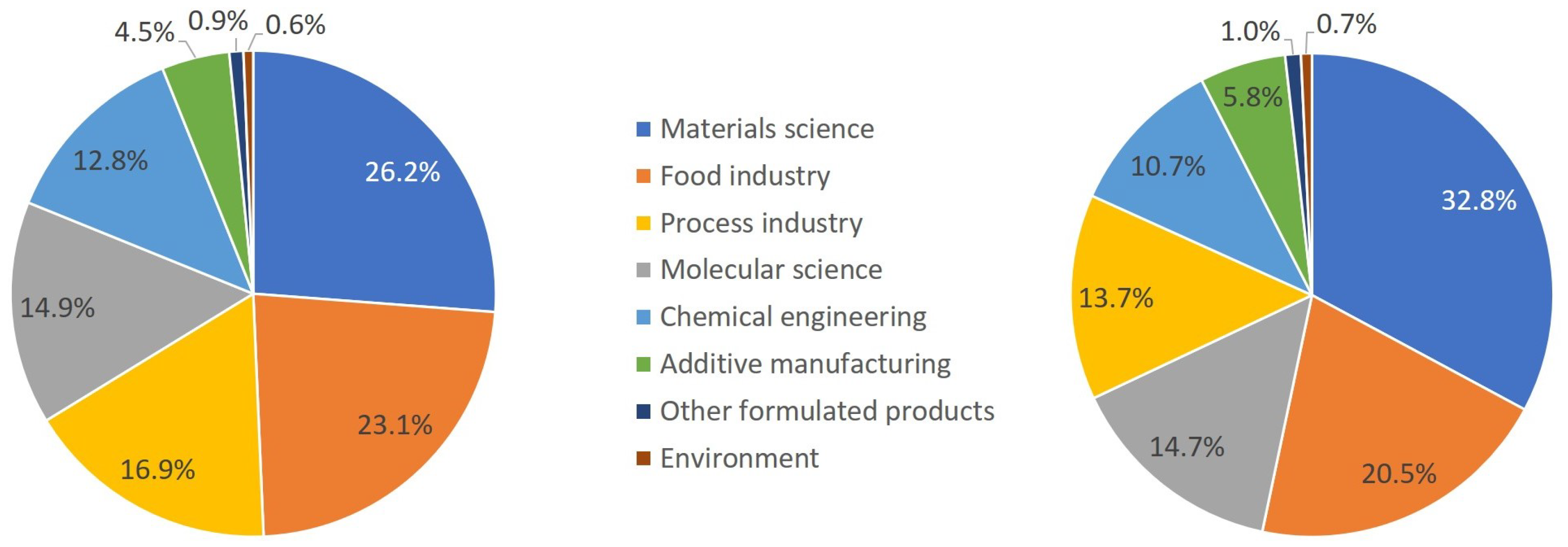
3.2. Overview of ML Methods in Chemical Product Engineering

This subsection provides a general overview of the ML methods that have been implemented in CPE problems from 2000 to 2021. After an initial exposition of the overall picture, the thematic area of CPE is further distinguished into a number of application domains, such as molecular and materials science, polymer science, food industry, cosmetics and pharmaceutical industry and catalysis, and a number of relevant recent studies are reported for each domain. Given the huge amount of reported studies, as well as the expansion rate of the relevant literature (cf. Figure 1), it is virtually impossible to cover the subject exhaustively in a single review publication.

The reported data in this section are based principally on the analysis of approximately 150 selected articles and review articles, published in the aforementioned period, and their respective references (i.e., a total of approximately 1500 references). Overall, this literature review pointed out the prevailing use of supervised learning methods in CPE, occupying an overall percentage of the reviewed reports of 69% (Figure 2). Hybrid, unsupervised learning and combinatorial methods displayed also significant applicability, as they were found to be implemented in 11%, 10%, and 7% of the reviewed articles, respectively.

At the same time, the implementation of semi-supervised learning methods (2%) and reinforcement learning methods (<1%) is thus far marginal in these application domains. These findings are consistent with the reported observations of other reviews, which also emphasized the major use of supervised learning methods compared to unsupervised learning methods in CPE or chemical engineering problems [2,21,26,70]. The interest in semi-supervised methods appears to be quite recent and displays an increasing trend, showing that this category of ML methods may become more significant for problems in the domain.

Figure 3, Figure 4 and Figure 5 describe, respectively, the distribution of supervised, unsupervised and hybrid methods in CPE applications. The most popular supervised learning algorithms are ANN, SVM/SVR, RF/DT, GP and kNN at, respectively, 35%, 20%, 12%, 8% and 5%, while the most popular unsupervised learning methods are PCA, ANN, ICA, GMM and k-means clustering at, respectively, 36%, 12%, 10%, 9% and 7%. As for hybrid methods, knowledge-based techniques are mainly combined with ANN, SVM/SVR, MR, partial least squares (PLS) and GP, representing, respectively, 44%, 8%, 6%, 5% and 4% of the applications. Figure 6 displays in which CPE sector ML techniques are most employed within the reviewed literature.

When considering all ML categories (left figure), the prevailing sectors are materials science (26%), food industry (23%), process industry (17%) and molecular science (15%). As for supervised learning methods (right figure), they are predominantly applied in the same sectors with slightly different percentages. Figure 7 depicts, in more detail, the type of problems that are principally solved using supervised (top figure) or hybrid approaches (bottom figure), namely modeling; optimization; control and monitoring; design and discovery; support to sensorial analysis; and reaction prediction. As for unsupervised methods, they are mostly used for dimensionality reduction, data visualization and information extraction.

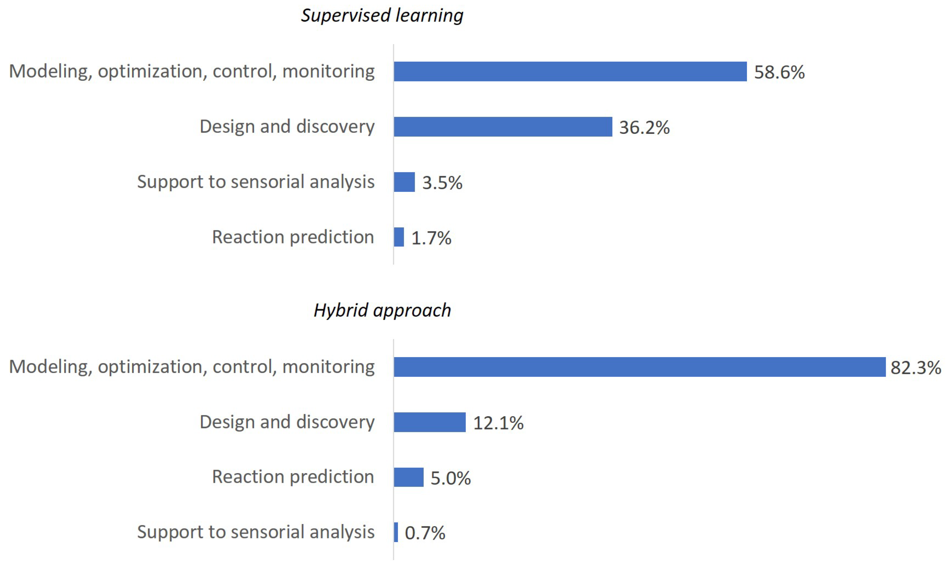
3.3. Popular ML Applications in Chemical Product Engineering Problems

• Design and discovery of new molecules and materials

One of the major applications of ML in CPE is the design and discovery of new molecules and materials referring, respectively, to the understanding and/or optimization of structure/property relationships, as well as to the exploration/screening of the large and high-dimensional chemical space with high throughput/autonomous techniques. Computer-aided techniques have shown their efficiency in these applications: for example, many organic chemicals-based products can be routinely designed through structure–property relationships [72].

However, as the chemicals are becoming increasingly complex, the existing models are not applicable anymore, and developing new models is costly and time-consuming as it requires establishing sufficient theoretical knowledge. For example, quantum mechanics (QM) methods (such as density functional theory (DFT) or semiempirical methods) or group contribution (GC) methods, which are commonly employed to calculate physicochemical properties, have shown limitations in their applicability to more complex and larger chemicals, which is often associated with their high computational costs [60,80,81].

As a result, new molecules and materials are often developed based on expert knowledge or trial-and-error experiments [75]. Nevertheless, ML methods could greatly help to extract quantitative structure–property or structure–activity relationships (QSPR or QSAR) from the collected data in cases where knowledge-based methods are limited [72].

The authors in [82,83] described the typical computational workflow for chemoinformatics QSPR-QSAR analysis using ML. This multi-stage processing is necessary as a chemical structure has to be converted into chemical information applicable for ML tasks. Thus, the first step is the encoding of the chemical structure, which consists of generating chemical descriptors (also called features) from the chemical structure. These descriptors are typically constructed in the form of chemical graphs, connection tables, linear text-based notations (e.g., SMILES, InChI and SMARTS) or fingerprints (i.e., vectors that indicate the absence or presence of a structural fragment/property) and contain the necessary information to provide as input to the model.

Additional details about these forms can be found in dedicated reported reviews, for ML applications [10,84,85,86,87]. This initial encoding stage is often carried out with the aid of specific software packages, such as PaDEL and Python RDKit, which are open-source and publicly available.

The generated descriptors can vary from a simple molecular formula to complete 3-dimensional chemical conformation descriptors, including molecular weights, functional group counts, structural topology and geometry, hydrophobicity, solubility and electronic and steric properties, whose values may have been theoretically determined or experimentally measured. Deep learning (DL) methods (e.g., autoencoder/decoder, adversarial and convolutional neural networks (CNNs)) have greatly simplified the problem of generating mathematical descriptors to train ML models as they can transform simple representations of molecular entities (e.g., SMILES strings and linear text representations of organic molecules) to relevant descriptors internally [9]

The generated descriptors will usually contain “too much” information, with respect to the requirements of the modeling of a specific SPR/SAR. Hence, the second step in this ML workflow typically consists of a feature selection step by means of an unsupervised dimensionality reduction algorithm. This enables identification of the most significant features, from the high-dimensional features vector, to reducing the computational cost of the final step and to increasing the efficiency and the accuracy of the model. The last step is the learning phase where the mapping between the significant features (x) and the properties of interest (y) is established using a supervised learning algorithm. Examples of algorithms in such applications include Naïve Bayes, MR, kNN, RF, SVM and ANN.

Compared to physical models, such as quantum chemistry (QC), molecular dynamics (MD) simulations or early QSPR-QSAR methods, ML methods are more suitable for exploring non-linear SPR-SAR with high accuracy and precision, compared to DFT calculations, without necessitating any prior knowledge of their functional form. ML methods are also faster than DFT calculations by many orders of magnitude, thus, reducing the prediction horizon from several hours (or even days) to a few seconds [10].

This allows a significant acceleration of the discovery process, since the development of new materials via the conventional trial-and-error procedure requires several months, with the synthesis step being the major bottleneck [88,89]. Finally, ML methods are easily scalable to big data sets, such as libraries with large amount of candidates, without the requirement for extensive computational resources. A schematic summary of the materials discovery workflow in the age of AI was also given by [10].

There are two types of problems that can be formulated in the framework of QSPR/QSAR, namely the direct or forward design problems and the inverse design problems. The forward design relies on the prediction of targeted properties of molecules or materials, given their structure and descriptors. This is a typical straightforward modeling approach that follows the classical paradigm adopted also by other modeling techniques. The inverse design problem is formulated as the identification of the most-likely candidates that are prone to possess a targeted property value (or a set of properties/values).

This problem, which would be commonly formulated as a model-based optimization problem in the case of a phenomenological model, can be treated directly in the framework of a supervised ML approach by inverting the inputs and outputs of the model. In both cases, an experimental validation of the identified materials is necessary at the end of the procedure. The difficulty in modeling QSPR/QSAR depends partly on the molecule/material complexity. Indeed, complex materials are harder to study compared to small organic drugs or drug-like molecules.

For example, nanomaterials present distributions of shapes and sizes, the surfaces change dynamically depending on the environment in which they are embedded, and materials are often not well characterized [9].

Table 3. Applications of ML in the design and discovery of molecules/materials. Acronyms: AAE: adversarial autoencoder, ANN: artificial neural network, BL: Bayesian learning, BNN: Bayesian neural network, BO: Bayesian optimization, COSMO-RS: conductor like screening model for real solvents, DFT: density functional theory, DNN: deep neural network, GAN: generative adversarial network, GP: Gaussian process, GCPR: G-coupled protein receptor, LASSO: least absolute shrinkage and selection operator, LDA: linear discriminant analysis, MR: multivariate regression, NLP: natural language processing, PCA: principal component analysis, QM: quantum mechanics, RI: refractive index, RF: random forest, RL: reinforcement learning, RNN: recurrent neural network, SMILES: simplified molecular input line entry specification, SVM: support vector machine, and VAE: variational autoencoder.

References	ML Method	Inputs	Outputs	Data Set
• Forward design (property/activity prediction from chemical structure)
[90] Fragrance	LDA, SVM	Molecules structural descriptors	Fragrance class (apple, pineapple, rose)	91 organic compounds with their fragrance class from database
[91] Cosmetics	ANN	Peptides	Anti-age properties	Data set from papers and patents (unstructured data) and from public databases (structured data), processed respectively by NLP and graph-based techniques
[92] Polymers	PCA/LASSO for data visualisation and feature reduction + GP for regression	Polymer relevant features	Refractive index (RI)	500 polymers from publicly available sources with their experimentally measured RI
[93] Polymers	GP + Lower confidence bound Bayesian optimizations	Molecular traceless quadrupole moment, molecule average hexadecapole moment	Glass transition temperature	60 polymers with their transition temperature from database
[94] Homogeneous catalysis	Hybrid: MR, Kernel ridge regression, RF, ANN and QM/DFT calculations	Energy, atomic, molecular, vibrational, structural descriptors (DFT)	Catalytic activity, reaction yield	4600–18,062 catalysts/reactions from libraries
[94] Heterogeneous catalysis	Hybrid: ANN, MR, RF, SVM, GP and QM/DFT calculations	Fingerprint features, structural and charge descriptors (DFT)	Adsorption, formation, binding, activation, reaction barrier energies, catalytic activity (DFT)	315–788 catalysts/reactions from libraries
[87] Molecules	Generative model for latent space creation (RNN, VAE, AAE, GAN, RL, BL and BNN) + predictive model for mapping latent variables and properties (RNN, RL, DNN, SVM, GP, BO and BNN)	Molecular representations (numerical, text-based or graph-based)	Physical, chemical or biological properties	5k–1800k molecules from databases
[67] Polymers	PCA/LASSO for data visualization and feature reduction + GP for regression	53–57 Relevant features from three hierarchical levels (atomic, block and chain)	Frequency-dependent dielectric constant, glass transition temperature	738 polymers and their 1210 experimentally measured properties at various frequencies
[95] Pharmaceutical compounds	GP and ant colony optimization algorithm (activity prediction followed by automated top scoring compounds picking from virtual combinatorial library)	Structure	Activity of ligand binding to 11 pharmaceutical relevant GCPRs (G-coupled protein receptor) drug target	3519 compounds with affinity annotations for 11 diverse GCPR targets (from libraries)
[83] Pharmaceutical compounds	ANN	Small molecules conformations	Energy of much larger systems	22 M small molecules conformations
[96] Polymers	GP (Polymer Genome)	Structure	Gas permeability	315 polymers and their associated 1501 permeability data
[97] Ionic liquids	ANN, SVM	Groups present in ionic liquid molecule	CO${}_2$ solubility	10,116 CO${}_2$ solubility data in various ionic liquids
[80] Cosmetics	Graph machine; Hybrid: ANN and COSMO-RS	SMILES, moments (COSMO-RS)	Viscosity	300 liquid compounds with known viscosities
[98] Polymers	GP, ANN, Kriging (Polymer Genome)	Polymer name, SMILES	Polymer properties	80–6721 polymers and associated properties obtained from first principles and experimental measurements
• Inverse design (generation of candidates molecules/materials given target properties)
[88] Polymers	ANN	Lightweight, strong, chemical resistant	Candidates structures/patterns	Large database from experiments and simulations
[99] Ionic liquids	ANN	Ionic liquid maximized solubility	Top ionic liquids candidates for CO${}_2$ capture	10,116 CO${}_2$ solubility data in various ionic liquids
[100] Molecules	ANN SVM and Kernel ridge regression	Specifications, properties, reagents	Candidates (structures and products)	Not identified

presents some examples of ML applications in direct and inverse design while

Table 4. Other applications of ML for the design and discovery of diverse molecules/materials.

References
[101] Polymers
[102] Thin film nanocomposite membranes
[103] Heterogeneous, multicomponent materials
[104] Memristors materials
[105] Thermal functional materials
[106] Mechanical metamaterials
[107] Energy materials
[108] Photonic crystals
[109] Metal-organic nanocapsules
[110] Hydrogels
[111] Renewable energy materials
[112] Alloys
[113] Functional materials
[114] Polymers
[115] Ultraincompressible, superhard materials
[116] Materials for clean energy
[117] Photo energy conversion systems

provides references of ML applications for the design and discovery of various molecules and materials.

• Prediction of chemical reactions and retrosynthesis

Reaction prediction (or forward reaction prediction) and retrosynthesis represent two of the main challenges of organic chemistry as they require chemists to have years of expertise. In a similar principle as in the direct and inverse materials design problems, the forward reaction prediction consists of predicting products given the reactants, reagents and reaction conditions. Inversely, retrosynthesis is the opposite procedure in which one seeks to predict the required reactants for the synthesis of a given product. The two problems are closely related, since a successful reaction prediction system can be used to validate a retro-synthetic proposal [118].

However, retrosynthesis is much more complex than forward prediction as several potential reactant combinations may lead to the synthesis of the same product (i.e., the equivalent of an optimization problem presenting multiple minima in the design space). Accordingly, this procedure is also often recursive until commercially available reactants are identified. The prediction of the reaction conditions (i.e., catalysts, reagents, solvents, temperature, pressure etc.) is also a challenge as the formulated multi-parametric design space presents the same characteristics as previously (i.e., multiple minima, discontinuities and high irregularity).

Overall, three different approaches have been used to computationally solve these two problems up to now, namely physical-based methods, rule-based experts systems and ML methods. Physical-based methods are based on simulations of the chemical reaction transition-state energies, primarily using QM. These methods result in very accurate predictions and provide in-depth understanding of the system but suffer from high computational costs and are limited to small molecules. Rule-based expert systems are computationally cheaper and have been very popular. They consist in establishing decision-making rules of human chemists using libraries of graphical rearrangement patterns or templates of chemical transformations.

However, they require a continuous time-consuming follow-up and update after any extension or modification of the database or the identification of a new rule or a conflict. Conversely, template-free methods are fully data-driven as no reaction templates are necessary. In this respect, ML methods can provide an interesting alternative, capable of responding to the aforementioned limitations, as they only require examples of reactions instead of encoded rules by experts and can significantly compress the simulation time. At the same time, their successful implementation depends highly on the availability, quantity and quality of relevant data.

Several sources of reaction information can be found in databases (not all publicly available), such as Reaxys, SciFinder, CAS, SPRESI, Beilstein and USPTO as well as the one from Lowe. For example, the latter is open-source and contains data for 1,808,938 reactions extracted from US patent grants and applications from 1976 to 2016 [119]. Another drawback in the application of ML methods in this domain is related to the fact that data sets include, as a majority, high-yielded reactions and only a limited number of negative examples of low-yielded or failed reactions, thus, severely biasing the available information that can be extracted from them. A comparison of the three approaches is given in

Table 5. Comparison of the three major approaches in reaction prediction and retrosynthesis.

Method	Advantages	Limitations
Physical-based	Accurate and generalizable Deep understanding of chemistry	Not adapted for high-throughput reaction prediction tasks and large systems (computationally expensive)
Rule-based expert systems	Computationally cheap/quick prediction	Requires a continuous time-consuming follow-up and update after any extension or modification of the database or the identification of a new rule or a conflict Not generalizable (i.e., not encoded chemistry will not be predicted by a rule-based system)
Machine learning	Only needs examples of reactions (i.e., no encoded expert knowledge required) Low computational cost Not limited to small molecules	Lack of sufficient high-quality and publicly available data Lack of negative examples (i.e., failed or low-yielded reactions)

.

Similar to the case of material design problems, the implementation of ML methods for the prediction (or retrosynthesis) of chemical reactions requires that the information extracted from the databases is transformed to a machine-readable format, before being injected to the model. To this end, molecular descriptors (structural, physico-chemical, electronic, topological) are once again employed in an adapted format, to describe the complete reaction procedure (in contrast to the description of a single molecule).

An example of such a reaction representation is via the use of reaction “fingerprints”, defined by the difference of the respective descriptors of the reaction products and reactants. These so-called fingerprints are vectors of binary digits that describe the presence (1) or absence (0) of a certain group or substructure on the molecule. The most popular ML techniques used in reaction prediction and retrosynthesis are ANN and DL, as they are specifically suited for recognizing nonlinear relationships within large and diverse data sets.

Contrary to some early attempts based on expert systems that did not lead to practical applications, ML has been increasingly applied to support experts in reaction prediction and retrosynthesis over the last decade. In particular, there have been noteworthy contributions from the teams of Kayala [118,120], Coley [23,121], Segler [122,123,124] and Schwaller [119,125,126,127]. The authors in [24] provided an excellent review that was specifically focused on the state of the art in reaction prediction and retrosynthesis. It is expected that ML will be of great help in this area for reducing the time-consuming and costly experiments needed for validating a synthetic route. Various applications of ML in reaction prediction and retrosynthesis are given in

Table 6. Applications of ML in reaction prediction and retrosynthesis. Acronyms: ANN: artificial neural network, DL: deep learning, GCN: graph convolutional network, HNN: hierarchical neural network, and SMILES: simplified molecular input line entry specification.

Application Category	References	ML Method	Inputs	Outputs
Reaction conditions prediction	[128]	HNN (classification and regression)	Reaction (difference between reactants and products fingerprints)	Reaction conditions (catalyst, solvent, reagent and temperature)
Ranking templates	[122,129,130]	ANN/DL/GCN (classification)	Reactants, reagents or product fingerprints	Most probable reaction template
Generating products	[119,131]	ANN/DL (encoder/decoder translation model)	Reactant SMILES	Product SMILES
Classifying reaction feasibility	[124]	ANN/DL	Product	Likely reactions
Predicting mechanistic pathway	[118,120]	ANN	Reactants, conditions, products	Reaction, mechanistic pathway
Ranking products	[121]	ANN	Possible reactions given reactants	Major product

.

• Modeling and optimization of process–properties relationship

Formulated and functional product properties are highly dependent on the prevailing process conditions during their synthesis and/or transformation steps. As a result, modeling the process–properties relationship is of paramount importance in CPE to ensure product quality and optimize production. The same general principles apply in this case as well; depending on the specific characteristics and complexity of the process, sufficiently accurate phenomenological models may exist or not, thus, making the necessity to resort to alternative data-driven models more or less pronounced.

Other factors playing a crucial role in this decision are the existing knowledge of the phenomena and the mechanisms governing the process, as well as the available resources in terms of time and/or budget limitations. Finally, data-driven techniques can be considered of specific interest, even in the case of existing knowledge-based models, when the simulation time is of importance (e.g., for online applications and optimization studies) or when the latter ones are highly dependent on ambiguous assumptions or on experimental characterizations that are difficult to acquire.

The state of the art highlights numerous applications of ML, especially in regression problems, for the prediction of product properties given the processing conditions. The inverse procedure, i.e., the prediction of processing conditions given the target properties is also encountered but less frequently, thus, providing the advantage to avoid complex inverse modeling and optimization procedures. Examples of applications of ML in process–properties modeling are summarized in

Table 7. Applications of ML in process–properties modeling. Acronyms: ANN: artificial neural network, C2V: code2vect, CFD: computational fluid dynamics, DBN: deep belief network, DoE: design of experiments, DT: decision tree, GP: Gaussian process, iDMD: inspired by dynamic model decomposition, LMNNR: large margin nearest neighbor for regression, MR: multivariate regression, PCA: principal component analysis, RF: random forest, sPGD: sparse proper generalized decomposition, and SVM/SVR: support vector machine/regression.

References	ML Method	Inputs	Outputs	Data Set
Polymer science
[136]	ANN	Dwell time, oven temperature, tension applied on filaments	Yield, final properties of carbon fibers	Not identified
[39]	Semi- supervised: DBN and kernel learning	Reactor pressure/temperature, liquid level and catalysts flowrate	Melt index	1900 unlabeled + 310 labeled
[137]	ANN	Process parameters	Monomer conversion, average molecular weight and viscosity, reaction time, dispersion and thermal stability	Not identified
[138]	SVM	Temperature, feed rates, reaction time and catalyst quantities	Viscosity	120 labeled
[139]	ANN, SVR, GP	Injection speed/pressure, packing duration/pressure, mold temperature, cooling time, shot size, screw rotation speed, cylinder pressure, barrel temperature, coolant temperature and sensor measurements	Product quality (deformation, defects), melt state, process parameters, fiber orientation distribution, physical/mechanical properties, skin layer and surface roughness	Not identified
[35]	PCA + GP	Hydrogen concentration, feed rate and reaction temperature	Process conditions and product quality	300 labeled
[140]	ANN	Temperature and clay composition	Dynamic mechanical properties (storage modulus and loss tangent)	More than 1500 labeled
[141]	GP	Process parameters (position, constriction angle, channel width, polymer and solvent flows)	Product parameters (median length, median diameter and quality of fibers)	Not identified
[142]	ANN, C2V, sPGD, SVM, DT and iDMD	Material and process parameters (rotation speed, exit flowrate, temperature and compositions)	Properties and performance (Young modulus, yield stress, stress at break, strain at break and impact strength)	59 labeled
[61]	Hybrid: knowledge-based and C2V and sGPD	Flowrate and rotation speed	Torque, pressure, engine power and exit temperature	47 labeled
[133]	LMNNR, Nearest Neighbor Regression with adaptive metrics	Reation conditions (initiator concentration, temperature and time)	Monomer conversion and average molecular weight	337–414 labeled
[62]	Hybrid: knowledge-based and ANN	Reation conditions (initiator concentration, temperature and time)	Monomer conversion and average molecular weight	3363 labeled
[143,144]	ANN	Reation conditions (initiator concentration and temperature)	Monomer conversion, average molecular weight and mass reaction viscosity	Not identified
Food industry
[54]	Hybrid: knowledge-based and SVR, SVM or ANN	Easy measurements (massecuite temperature/volume/level, vacuum degree, steam pressure/temperature and feeding rate)	Difficult measurements (mother liquor purity/supersaturation)	210 labeled
[56]	Hybrid: knowledge-based and RF	Food ingredients (selection and composition), processing conditions (baking time and temperature)	Sensory properties (color, crispiness and flavors)	446–462 labeled
[66]	Hierarchical clustering	Intrinsic characteristics of yogurt product	Brand and storage conditions	36 unlabeled
Pharmaceutical industry
[145]	ANN/Fuzzy logic	Flowrates, frequency of vibration and concentrations	Microparticles properties (shape, oil content and distribution)	41 labeled
[146]	ANN/Fuzzy logic	Compositions, stirring speed	Properties of nanoparticles (size, size distribution, zeta potential, encapsulation efficiency and drug loading)	15 labeled
[147]	MR	Base equivalents, water equivalents and solvent loading	Dynamic profile of starting materials, product and key impurity	25 labeled
[148]	CFD and DoE and ANN	Dimensionless parameters based on material properties, concentration of the particles, viscosity of the injection solution and ratio needle diameter over the greatest dimension of the particles	Drug injectability	319 labeled
Paints
[149]	ANN, MR	Formulation parameters	Thermodynamic and functional properties (elasticity, hardness and barrier properties)	Not identified
Catalysis
[150]	ANN	Nominal silver concentration, pH, reaction time, actual amount of Ag attached on ZnO surface, initial contaminant concentration and light wavelength	Actual amount of Ag attached on ZnO surface and photodegradation performance	27–63 labeled
Minerals
[132]	PCR	Fast and easy measurements (flowrate, pressure, temperature and spectra)	Slow and difficult measurements (composition, size distribution, mill load and equipment failure)	Not identified
Textile
[151]	ANN	Process and structure parameters (bleaching or dyeing, bio-polishing, softening, emerizing, calendering, material and count of yarn)	Sensory properties (bipolar, surface and handle attributes)	23 labeled
Materials science
[152]	SVR, ANN	Structure and process parameters (temperature, stretching ration and space velocity)	Mechanical property (Young’s modulus and tensile strength)	30 labeled

for various domains, such as polymer/material science, catalysis and the food/pharmaceutical/mineral/textile industries.

Depending on the application domain, diverse target properties are also predicted, including mechanical, structural and sensory properties, with respect to different process conditions, such as the temperature, time and composition. The sizes of the datasets used in these applications are relatively limited (i.e., typically inferior to 100 data) compared to other applications of ML. For example, in the aforementioned application domain of reaction prediction and retrosynthesis, the size of the databases ranges from several thousands to a few millions of reaction data. This is mainly due to the difficulties associated with the realization of experimental measurements in order to acquire the relevant process–properties data, which are time-consuming and costly.

These difficulties have also given rise to ML applications in soft sensor problems, which consist in predicting quality variables that are slow and/or difficult to measure directly, via the use of alternative process measurements that are faster and easier to acquire [54,132]. For example, in industrial polyethylene polymerization processes, it is more interesting to relate the measurement of the melt index of the produced polymer, which is normally analyzed offline every several hours, with alternative process variables, such as temperature and pressure, which can be readily measured online with high frequency [39].

Another reason for this lack of abundance of representative data is related to the discontinuous nature of the processes that is often encountered in CPE, where the production specifications are frequently modified to manufacture products of different grades and with different properties. To overcome these limitations, larger data sets can be obtained directly from simulations (hybrid methods) [62,133], publicly available databases for the same system [56] or exploitation of relevant unlabeled data in combination with a semi-supervised ML method [39].

The polymer industry has a large number of ML modeling applications to display, within a process–properties relationship context, mainly due to the nature of the polymer molecules that are inherently complex (i.e., in terms of their macromolecular nature and diversity of structures and conformations). Indeed, the quality of a polymer product depends on a wide range of morphological and molecular properties, with direct implications for its end-use properties (i.e., physical, chemical, thermal, rheological and mechanical) and applications [134].

However, other important difficulties, specific to the polymerization processes, also explain the interest in ML techniques. Polymerization systems are commonly marked by a significant increase in the viscosity of the reaction medium, by several orders of magnitude, along the reaction, with direct implications on the control of the prevailing heat transfer rates as well as on the very mobility of the different macromolecules, thus, affecting the reaction rates. The mechanistic modeling of polymerization reaction kinetics can be extremely complex and time-consuming depending on the system. Indeed, these models contain a large number of differential equations, complex reactions occur simultaneously and many kinetic variables can be unknown or difficult to determine precisely.

In addition, the properties of the produced polymer products can be modified at-will by the addition of diverse materials, such as fillers and reinforcing agents, during different steps of the process. An example is the use of recycled tire powder to modify the mechanical properties of polystyrene [135]. Although the kinetic modeling of styrene radical polymerization is well-documented and relatively trivial, the presence of the recycled tire powder of variable composition in the system brings about a series of diverse effects on the evolution of the kinetic developments that are difficult to describe due to the current limited understanding of these mechanisms.

• Support for sensorial analysis

Sensory evaluation has been widely applied in diverse industries, such as the food, cosmetic and textile industries for quality inspection, product design and marketing. Indeed, these industries have to propose diversified products that satisfy consumer preferences, and sensory attributes represent important factors to assess the quality and market acceptance of consumer goods. While appearance is rather easy to evaluate, the sensory qualities of a product are more difficult to evaluate, and its assessment is, therefore, a challenge to ensure high quality products. Up to now, the common practice to evaluate sensory attributes and to predict customer responses is through sensory panels, composed of humans (experts or not and trained or not), whose evaluation is considered representative of the general target population [153].

In this respect, the members of the panels use their senses to assess sensory properties, such as the color, aroma, taste of a product and skin feeling. However, sensory panel evaluation exhibits several drawbacks in terms of resources (costly, time-consuming, necessity to train some panels, a well-defined procedure to guarantee same sensory conditions for all panelists…) and also in terms of data characteristics and quality. In particular, data in sensory evaluation is subjective and uncertain and can contain inherent sources of misinterpretation (e.g., linguistic expressions) [154,155]. There is a general lack of reproducibility, standardization of the measurements and comparability between evaluations of different panels [156]. All these reasons make sensory panel assessments ill-adapted to routine quality evaluation.

The state of the art highlights diverse applications of ML methods to assist the complex sensory evaluation of products, with a specific emphasis on food products, and to study the impact of process, microstructure or chemical compositions on sensory attributes. Accordingly, ML methods have been increasingly applied in problems where more classical methods, deriving from the field of chemometrics, were typically implemented. Chemometrics uses multivariate analysis and statistical methods, such as analysis of variance (ANOVA), PCA, partial least squares (PLS), MR or principal component regression (PCR), to analyze multivariate data, instrumental or not.

Chemometrics methods, such as ANOVA or PCA, are most often applied before ML methods to select and compress the original data [156,157,158,159,160,161,162,163,164]. Feature extraction methods such as Fourier analysis or Si-PLS are also used for extracting relevant information or optimal spectral interval from high dimensional spectra measurements [156,158].

This step is particularly important when working with spectral data as it prevents many irrelevant or redundant spectrum variables from being introduced and, therefore, decreases the complexity and size of the variable space and improves the precision of the model [164]. Supervised ML methods, such as ANN, SVM and RF, are then applied to link the sensory properties with the process parameters, the ingredients or the microstructure of the tested products.

Several works compare the use of AI techniques and classical approaches. The authors in [155] compared the uses of classical computing techniques, mostly based on statistics and multivariate analysis (PCA, generalized procrustes analysis and generalized canonical analysis), with AI in sensory evaluation. They found that AI methods had better ability in solving specific and human-related problems using both linguistic and numerical data processing.

They can also take into account nonlinear relationships as well as the specificity of sensory data and uncertain evaluation conditions. In another study, the authors in [159] used SVM and concluded that regression methods, such as PLS, were not able to capture consumer preferences, due to the so-called “batch-effect” which was not compatible with the consideration of the consumer ratings as absolute assessments. In other words, the ratings should be treated as relative data, in relation to the rest of the evaluated objects in the same “batch” of the sensory analysis.

Great effort in sensory evaluation has been made in an attempt to replace the subjective sensory evaluation with the use of more objective, robust and reproducible instrumental and analytical measurements, in view of overcoming the associated uncertainty, imprecision and time demand of the classical sensory evaluation procedures [155,164]. Analytical methods, such as near infrared (NIR), Fourier transform infrared (FT-IR) and Raman spectroscopy analyses, or other instrumental methods combined with ML or chemometrics algorithms, have been used as efficient methods to quickly evaluate the biochemical or physical characteristics of food products and decode their correlations to sensory attributes.

The authors in [157] successfully applied ANN to predict chocolate physico-chemical properties and sensory descriptors based on specific absorbance values of NIR spectra. This rapid (one spectral measurement takes only 15 to 90 s) and non-destructive method represents an alternative to consumer panels in determining the sensory properties of chocolate in a more accurate, cheaper manner using chemical parameters. In another application, the authors in [158] reported a sensory analysis of puffed snacks crispiness-related freshness level, for various humidity levels, via the recording of mechanical and acoustical data.

In this study, ANN and SVM were selected for their ability to provide models that are more similar to the way sensory integration takes place in humans, in comparison with algorithms relying on linear relationships. Contrary to that, [158,165] opted for the implementation of RF for predicting wine olfactory characteristics from the volatile organic compound content as measured by gas chromatography–mass spectrometry (GC-MS), in order to gain interpretability in the final model.

ANN has also been employed, in combination with AdaBoost, to improve the prediction performance of the sensory attributes of rice wine from the NIR spectra [156]. The authors in [153] combined PLS regression and SVM to predict pork meat sensory attributes (tenderness, juiciness and chewiness) and quality grade group, on the basis of Raman spectra, while [166] reported the development of an ANN-based predictive model of several sensory descriptors of beer, using NIR spectra.

The prediction of the smell impression from the physicochemical properties of a molecule represents an important breakthrough for the cosmetic, beverage and food industries. A large number of experienced panelists are usually needed to create the desired odors through trial-and-error approaches in these industries. At the same time, the mass spectra of physicochemical properties can be used to represent structural information of the constituting molecules of a product that can be correlated with its odor.

The dimensionality reduction step, in these applications, is often carried out via the use of non-linear ML methods, such as an autoencoders neural network (AENN), which prevents the loss of information compared to the aforementioned classical chemometrics techniques. The authors in [167] utilized an AENN in the dimensionality reduction process of mass spectra of molecules from the NIST (National Institute of Standards and Technology) database and performed the clustering of descriptors by natural language processing to predict the odor category of chemicals. The authors in [66] used AENN combined with SVM for the prediction of yogurt preferences using sensory attributes.

The authors in [164] compared several linear and nonlinear dimensionality reduction (kernel PCA, sparse PCA, local tangent space alignment, PCA and multidimensional scaling) and regression methods (relevance vector machine, back-propagation ANN and PLS) for estimating the sensory quality of tea from NIR spectra. In this application, nonlinear methods displayed better performance due to existing non linearity in tea components and NIR spectra. In addition, their increased performance was also attributed to the structure of human sensory organs that act as an extension of the highly-complex central nervous system, displaying high degrees of sensitivity and specificity.

Another application of ML methods in the field of sensorial analysis is to evaluate the impact of processing conditions on sensory drivers of liking. The authors in [162] used different ML techniques, namely RF, gradient boosted tree and extreme learning machine, to predict the sensory drivers of cheese manufactured with milk subjected to conventional thermal processing and to ohmic heating, an emerging thermal technology in the dairy industry. Hybrid approaches are also encountered in this field as well. The authors in [56] combined RF with mechanistic models to predict food sensory characteristics (color, crispiness and flavors) with respect to the ingredients (selection and composition) and the processing conditions (baking time and temperature).

In addition, in the food industry, where ML techniques find widespread application, the cosmetics and textile industries are also interested in similar ML and/or hybrid approaches to support sensorial analyses. For example, in the field of cosmetics, the authors in [168] employed an ANN-based surrogate model, as part of an integrated optimization-based cosmetic formulation methodology, including the implementation of mechanistic models and heuristics, to predict the sensorial rating of cosmetic products given their recipes and microstructures. The authors in [151] also used ANN and fuzzy logic for tactile sensory property prediction from the process and structure parameters of knitted fabrics.

The interest in ML for supporting sensorial analysis is expected to rise given its capacity in treating the associated complex interactions that impact product quality and sensorial attributes. A typical example concerns wine, where important quality traits, such as the sensory profile and color are a product of complex interactions between the soil, grapevine, environment, management and winemaking practices. ANN has been shown to be an efficient tool in assessing these complex interactions and predicting wine sensory properties from NIR spectra and from weather and water management information [163]. This example is illustrative of the way AI can present an opportunity for winemakers to adjust vinification techniques in order to obtain a more consistent wine style, predict market and consumer acceptance for pricing adjustments and provide better description of wines on labels for accurate information to consumers.

Finally, it is worth noting new emerging technologies that, combined with ML, enable performing analyses in a more standardized and rapid manner, such as robotic pourers with computer vision, electronic tongue or nose sensors or low-cost NIR spectroscopic devices and color sensors, attachable to smartphones with applications in food and beverages [163,169,170].

4. Guidelines for Applying ML in Chemical Product Engineering Problems

While the previously presented state of the art outlined the variety of ML methods applied in diverse applications of CPE for solving different types of problems, this section aims at providing some general guidelines for applying ML in relevant problems. In this respect, the principle of the most commonly encountered ML methods is briefly presented, along with their main advantages and limitations. Then, the discussion is extended to several aspects related to the interest of employing data-driven methods, the challenges that are frequently encountered in the process and some rules of thumb that may serve as indicators in the selection of the ML technique in relation to the problem characteristics and data configuration.

4.1. General Principle of Some Popular ML Methods in Chemical Product Engineering

According to literature review, most popular supervised ML methods in CPE seem to be ANN, SVM and GP. As for unsupervised methods, PCA is the most widely used.

• ANN

ANNs are widely encountered both in chemical engineering and in CPE problems. This is a family of methods that are based on the principle of the capacity of the human brain neurons to “learn” and repeat a specific action, given relevant stimuli as input. ANNs can be effectively considered as systems of interconnected calculation nodes, i.e., the so-called “neurons”, that exchange messages amongst them. A typical ANN generally consists of an input layer (containing a number of nodes equal to the number of input variables), an output layer (containing one or more nodes to represent the output(s)) and one or more intermediate layers in between (also called “hidden” layers).

Each of these intermediate layers is also composed of a number of neurons, which are connected to the neurons of the adjacent layers. Each connection is associated to a weight. A neuron is a processing unit, which transforms the input data (i.e., the sum of all inputs arriving at the neuron multiplied by their corresponding weights plus a bias term) to the output by an activation function. Examples of activation functions are given by [52].

The values of the network parameters (i.e., weights) are adjusted during the learning step on the basis of a set of training data through an iterative process of minimization of the distance between the predictions of the ANN and the responses (i.e., labels) of the data set. Common learning algorithms are Levenberg–Marquardt, gradient descent, quasi-Newton method (BFGS) and scaled conjugate gradient. The most important parameters to consider when designing an ANN are the number of hidden layers, the number of neurons in each hidden layer, the activation functions and the training algorithm.

Note that the number of neurons in the input and output layers are explicitly defined by the problem characteristics. The optimal network architecture, in terms of its number of layers and neurons, is usually defined based on a trial-and-error approach, by evaluating the performance of ANNs of different architectures. This evaluation is often based on the value of the mean squared error (MSE) between the network outputs and data set labels.

The role of the activation function of the hidden layer(s) is to introduce nonlinearity to the overall model, thus, increasing its capacity to simulate highly complex, non-linear response surfaces [152]. Accordingly, after the training step, the network can be used to perform diverse tasks, such as regression, classification and dimensionality reduction. ANNs may also include internal “recycle” connections (i.e., recurrent networks), providing them the ability to adapt better to dynamic problems and to time-series data. In addition, multiple “stacked” ANNs may also be combined, in different manners, to exploit the uncertainty in their predictions.

Finally, “deep” ANNs (i.e., “deep learning”) can also be constructed with the combination of several layers of sequential convolution and pooling operations, thus, allowing a more efficient feature learning process of highly-dimensional problems; however, their analysis exceeds the framework of this report. A more detailed description of the different types of ANNs (such as single or multi-layer perceptron (MLP), recurrent neural networks (RNNs) and convolutional neural networks (CNNs)) can be found in [25,30,52,171].

Although the exact form of the mathematical model that is produced by a neural network is quite complicated, as it contains a large number of terms (i.e., relevant to its number of neurons and connections), developing a NN model is greatly simplified by the use of a number of dedicated libraries and softwares (e.g., Matlab toolbox, Python-C++ Scikit-Learn/TensorFlow/Keras, R and Weka) that offer a more user-friendly way of handling them [172].

The power of ANNs resides exactly in their ability to approximate any linear/nonlinear function by learning from observed data, presenting, at the same time, inner structure flexibility, adaptability, and a dynamic nature. As such, they are commonly employed in problems where the form of the response surface is entirely unknown (i.e., a lack of previous knowledge) and/or displays a highly nonlinear, multi-dimensional (i.e., in terms of the features), complex nature.

ANNs bypass the necessity to explicitly define the nature of the terms of the derived mathematical model, as is commonly the case for classical experimental design data-driven approaches. At the same time, in order for a ANN to be sufficiently accurate, significant amounts of data are often required. In this sense, they are recommended mainly for applications in which large volumes of data are either available or easy to generate [10,173]. In addition, ANNs are also prone to overfitting, thus, requiring specific attention during the learning process (more details about the phenomena of over/under fitting of ML methods are given in Section 4.4), which also presents some inconvenience due to the existence of multiple local minima.

• SVM

SVM is another popular ML technique that is most commonly employed for classification analysis. The model finds the hyperplane that separates the input data into distinct classes in a way that the “margin” (i.e., defined by the decision boundary lines and containing the hyperplane in the middle) between the classes is maximized. To define this margin, SVM uses only those points, among all input data points, that are located closest to an eventual decision boundary. These are the so-called “support vectors”, explicitly dictating the optimal position of the separating hyperplane by maximizing the distances between them and the hyperplane. When a linear hyperplane (i.e., a line or a plane) is adequate to separate the classes, the model is linear.

In the opposite case, where the data cannot be considered as linearly separable, SVM can still be applied, in combination with a projection of the data set to a space of different dimensions (typically a higher-dimensional projection is employed), through the use of “kernels”. This mapping procedure transforms the data set into a linearly-separable one, thus, making the use of SVM again possible. There exist different types of kernel functions, such as Gaussian, polynomial, radial-basis functions and sigmoidal.

A major advantage of SVM, with respect to ANN, is its robustness in reaching a global optimum during the training (or learning) process. In fact, the problem of maximizing the margin is formulated as a quadratic constrained optimization problem, presenting a global minimum [26,174]. It can also perform with high precision and generalization with a small number of training samples, high dimensional and noisy data [52,152]. In fact, SVM uses a penalty hyperparameter to treat misclassification cases of noisy data, containing errors of labeling or outliers [31]. Among the drawbacks of the method is that its prediction performance is highly dependent on the suitable setting of its parameters, such as the kernel function, regularization parameter and insensitive loss function [174].

In addition to classification problems, SVM is also employed in regression problems, in which case it can also be referred to as support vector regression, SVR. The principle of the method, when applied to regression problems, is the same as in classification, i.e., a hyperplane is sought in this case as well. However, this time, the points that are considered lie within the decision boundary, and the goal is to have as many points as possible located on (or around) the hyperplane, which serves as the regression function. More details about SVM and SVR can be found in [25,30,31,175].

• GP

GP is a supervised ML method that has also been increasingly used in CPE for regression problems. GP is based on the description of a probability distribution over functions, defined by a mean function and a covariance matrix. Concretely, for a given set of training points, a typical regression procedure would require assuming the form of the function that best describes them before identifying the values of the parameters of this function. As ANN overcomes the difficulty that is posed when this functional form is unknown by employing a highly-complex mathematical expression to substitute it, GPs propose to select the best-fitting function out of a large number of different candidates.

In this sense, GP defines a prior over functions (i.e., a large number of candidate functions for the given problem) that is gradually transformed to a posterior over functions, once enough data have been presented to algorithm. GPs are considered to be “non-parametric” techniques, in the sense that their scope is to identify a specific set of parameters that are a priori posed by the form of a known function and, rather, to identify the function itself.

In order to define the probability distribution over functions (i.e., prior or posterior), GPs are based on the premise that these functions are jointly Gaussian, characterized by their mean and their covariance matrix. The mean represents the most probable output of the data, while the covariance serves as a measure of the smoothness of the functions [176]. Accordingly, two inputs that are considered similar (or close to each other) will also, most probably, produce similar outputs. GPs will, therefore, improve the confidence of their predictions as they receive new data, allowing them to better identify the posterior over functions, and new inputs that are similar to the existing ones.

As such, one of the great advantages of this method is its rigorous treatment of uncertainty, which helps in avoiding overfitting problems [177]. Its inherent preference to smooth functions is an additional factor that increases its generalization capacity, as fitting artifacts are avoided [176]. The probabilistic structure of GP can successfully incorporate the noise information and provide uncertainty prediction result (confidence interval) for the process, which is very helpful for quantifying prediction reliability in problems of evolving conditions or wide operating ranges [35].

Consequently, GPs are employed in numerous applications, in addition to typical regression problems, such as surrogate model identification, dynamic experimental design and manifold learning-based modeling [177,178,179]. On the other hand, a major drawback in the application of GPs is their high computational demands when dealing with large data sets [10,177,180]. In fact, as the implementation of the method requires the continuous manipulation of the covariance matrix, whose size is directly proportional to the size of the data set, the computational cost increases. As such, GPs are rather more adapted to problems involving small data sets, which is in contrast to ANNs that require abundant data. More detailed descriptions of GP can be found in [181].

• PCA

PCA is, by far, the most commonly used algorithm for dimensionality reduction problems. The aim is to transform the original set of variables to a new set of uncorrelated variables, called principal components, without significantly reducing the relevant statistical information contained in the data. As such, it aims at finding an optimal trade-off between information loss and simplification of the problem. The method is based on the principle of projecting data from a k-dimensional space to a n-dimensional one, thus, reducing the considered coordinates.

For example, when a set of data is projected from 2D to 1D, their surface is reduced to a single line, just as a projection from 3D to 2D reduces the “cloud” of points to a plane. Accordingly, PCA will identify k principal components, orthogonal to each other (i.e., uncorrelated), on which to project the original data, in a way that the projection error will be minimized. This error is defined as the sum of squares of the segments between each point and their projected counterparts. Once all principal components have been identified, a reduced number of them will be commonly retained for the rest of the analysis, while the rest will be ignored. This number will depend on the amount of statistical information they contain, described via the percentage of the total variance that they are able to explain.

This step of the selection of the main principal components is, therefore, crucial to the successful application of the method, since a low number of selected principal components may bring about a significant loss of information. Inversely, retaining too many principal components reduces the efficiency and the whole intent of applying PCA in the first place. Commonly considered thresholds for this selection vary between 90% and 99% of the total variance.

PCA is usually employed as a preprocessing stage on the data before a regression or classification problem. It is highly recommended for multi-variable/high-dimensional problems to reduce the computational time and memory demands and to avoid overfitting issues that may be caused by the consideration of an excess number of features, often correlated among them [26,65]. PCA is also very useful in visualizing high dimensional data sets (i.e., by plotting them with respect to the first two or three principal components), which turns out to be extremely helpful in better understanding the data set before applying an appropriate regression or classification technique.

The main limitation of PCA is that it performs linear transformation of the variables, thus, somewhat limiting its capabilities with respect to nonlinear dimensionality reduction methods, such as ICA. PCA is very well documented in several statistics textbooks and dedicated reports [25,30,31].

• Other ML methods

For more details on the previously described ML methods as well as other popular ML methods, a plethora of dedicated textbooks and articles is available in the open literature. In addition, over the last years, numerous online courses from highly recognized researchers and institutions have become freely available, serving as excellent entry points to the world of ML algorithms. An indicative list of such sources is given in

Table 8. Sources for an introduction to the fundamentals of ML algorithms.

MOOCs	Books, Articles
Machine Learning—Coursera	[30]
Deep Learning Specialization—Coursera	[31]
Machine Learning with Python—Coursera	[182]
Advance Machine Learning Specialization—Coursera	[25]
Machine Learning—EdX	[175]

.

4.2. Interest of Data-Driven Methods

Given the popularity that ML methods have gained over the last years, their implementation to problems has become a standard. Indeed, increasing researchers are tempted to apply ML techniques, driven either by their popularity or their undeniable capacities. However, ML methods are not always interesting to apply in all problems, nor are all types of ML techniques adapted to all kinds of problems [30,182].

A very good reason to resort to data-driven techniques in general or to ML techniques in particular may be related to a substantial lack of knowledge and understanding of the mechanisms underlying a system or process, in combination with the lack of resources (i.e., in terms of time, budget, personnel, infrastructure etc.) to seek this knowledge via phenomenological approaches. For example, in sensory evaluation, the problem of linking process parameters or ingredients to the sensorial properties involves the investigation of the unknown interactions of a large number of factors with each other, along with the understanding and description of their effect on the neurological responses of the human brain, a task that is still far from being trivial with the current scientific knowledge.

Another reason for opting for ML techniques may be related to the fact that the gain in understanding of the mechanisms is not difficult to reach but simply less interesting in comparison to other aspects of the study. Such aspects may concern the need for automation, speed or simplicity of the developed model. Accordingly, in the previously reviewed applications of chemical reaction predictions and retrosynthesis, the approach that is based on the coding of reactions rules is too laborious and limits the flexibility, automatisation and extensibility of these models to a point that it becomes more interesting to resort to data-driven techniques. ML can accelerate the prediction of the properties of new molecules, without the necessity to systematically make use of computationally expensive approaches, such as MD and QM methods.

Finally, ML techniques are specifically adapted in dealing with the complexity that is associated with multi-parametric, multi-dimensional, non-linear problems. The very fact that their operating principle is founded on the treatment of data makes them particularly suitable in identifying correlations and patterns that are distinguishable, or even comprehensible, by the human brain via mechanistic approaches. In this sense, their application to problems associated with the exploration of new domains and the seeking of unexploited information on the frontiers of scientific knowledge is specifically interesting. A typical example is the implementation of ML techniques for the analysis of new, unexplored areas of the chemical space for the discovery of new materials, molecules or reactions.

At the same time, ML methods possess their own share of limitations and drawbacks, both as a class of methods and as individual techniques, that must not be overlooked when considering their implementation to a specific problem. One of the most important issues is related to the availability, quantity and quality of data; however, this is addressed separately in a following section.

However, in a related topic, one must consider carefully the required resources, both for the data collection, cleaning and treatment, as well as the resources required for the training of the ML algorithm, which can be quite substantial in certain cases (e.g., in ANN and DL applications) before engaging in an ML application. In no case should ML methods (or AI methods as a whole) be considered “magic-tools” that will provide all the answers with the simple push of a button.

In addition to the above, ML methods, as data-driven techniques, inherit all the relevant drawbacks, such as poor understanding, as well as limited extrapolation capacities. As such, although they can be used to gain insight to the way different features affect an output or interact among them, they are not strictly capable of providing a deep understanding of the phenomena, the mechanisms and the driving forces behind the observations. Furthermore, their application domain is normally limited by the range in which the data set that was used for the training of the algorithm can be considered representative.

Any extrapolation outside this domain by no means guarantees equal prediction accuracy by the trained model. Accordingly, even though ML methods are often advantageous when applied to problems characterized by fluctuating conditions (e.g., in production monitoring for online quality control), due to their ability to quickly identify and adapt to the transitions in the input, this presupposes that these fluctuations have been, at a certain moment, part of the training data set that the model has “seen” before (i.e., in the case of supervised learning methods).

It is important to consider these aspects before implementing a ML technique to a given problem, in order to have a clear sight of the objectives of the modeling study, the capacity of the selected method (or combination of methods) to completely or partially contribute in reaching these objectives, as well as of the associated limitations and drawbacks of the developed model. This will eventually allow a maximum exploitation of the tremendous capabilities of these very powerful techniques.

4.3. Challenges and Solutions

Several challenges frequently encountered in ML applications in CPE are discussed in the following paragraphs, namely the availability and quality of data, the difficulty of chemical data representation and the lack of understanding. The initiatives implemented to address these challenges are also presented. Similar discussions about different application fields, such as synthesis planning, materials and drug discovery, can be found in other reported studies as well [11,23,183,184,185].

• Data

Any data-driven technique can only be as good as the data it uses. However, the choice of a representative data set of “good” quality and “sufficient” quantity is crucial to the performance and the reliability of the developed model. In computer vision and natural language processing areas, which have benefited from the AI-related research over the last decades, data are often abundant, publicly available and simple to acquire [79,186].

On the contrary, in CPE, data is more expensive to generate and rarely publicly shared due to confidentiality and competitiveness reasons. In addition, the uncertainty related to some types of generated data can be extremely variable, thus, creating additional drawbacks in their common utilization in shared databases. These elements are only some examples of the numerous challenges related to the data, as a constitutive unit of any ML application.

According to the above, the first big challenge concerns the data availability and extraction capacity. The scientific literature contains huge amounts of experimental and theoretical data in disorganized and unstructured forms, such as text, figures and tables. Since the task of efficiently extracting them in machine-readable form cannot be performed manually, text mining algorithms have been developed and are often used.

However, the lack of a generally-applicable standard along with the ambiguity and variability in the conventions that are met between different scientific domains (and even sometimes within the same scientific area), limit the universality of the developed dictionary and rule-based approaches [10]. Nuances of language and unconstrained diversity of figures and tables inhibit automated interpretation and extraction by text mining algorithms [186].

When data are obtained from experiments, their number is often limited. On the contrary, simulation-generated data or data registered in available databases (e.g., UPSTO for chemical reactions) typically reach much larger quantities. The availability of data is also more or less dependent on the application area. For example, publicly available data are less abundant in the organic materials and polymer research domains, compared to inorganic materials and drug design [10,68,79,187]. Examples of databases can be found for organic materials [10], inorganic materials [11], chemicals [87], materials [188] and molecules and solid materials [5].

This lack of data is quite frequent in CPE problems. To overcome this limitation, the scientific community is looking for ML methods that are specifically adapted to limited-data problems, such as kernel methods, low-variance models with feature reduction capabilities, multi-process modeling and transfer learning [189,190,191,192]. An example is given in [10], where a DNN, implemented in organic materials design, updates its initial weights from a large data set, derived from a similar domain to the target problem, and then fine tunes its weights using a smaller, dedicated data set, thus, learning the subtle characteristics that are specific to the targeted application.

Another approach to deal with this absence of large data sets is the implementation of semi-supervised learning techniques. Accordingly, unlabeled data can be pseudo-labeled by the ML model, established on the basis of the available limited amount of labeled data, thus, forming an augmented data set. Finally, active learning is another interesting technique that is frequently employed when the acquisition of labeled examples is expensive [11,173,193]. In this case, the model learning process initiates using relatively few labeled examples. At a second stage, the algorithm examines the obtained preliminary results and selects a sub-sample of the unlabeled data on the basis of their potential contribution to the learning process.

These are subsequently annotated, often by the intervention of human-experts or via classical experimental techniques, and the obtained samples are added to the labeled training set to rebuild the model. This cyclic procedure continues until some convergence criterion or limiting condition has been reached, such as a satisfactory model accuracy or a maximum number of annotations due to budget or time limitations [31,173].

Finally, it should be noted that the current trend in research, intensively promoted over the last years by numerous funding organizations and research institutions, encouraging data sharing within the scientific community, is expected to greatly improve the aforementioned limitations [187]. Other solutions for improving data-sharing practices, such as the use of publication standards, Google’s data set search or specialized consortium creations, are also evoked [186].

In addition to their availability, another significant issue is the quality of the data. A typical example is found in the area of chemical reaction prediction and retrosynthesis, in which applications of ML are relatively recent. The available data are often incomplete, especially with regards to the reactions conditions (i.e, solvents, temperature and catalysts), which are not always specified, despite their significance to the reaction output (i.e, products and yield of the reaction). In addition, databases contain principally high-yielded reactions, while failed or low-yielded reactions are often not reported as they are considered “failed” attempts.

However, these “negative” data contain a wealth of information that is as important as the “positive” data, since they can serve in the identification of undesired domains of the feature space (i.e., in contrast to leaving this space largely non-characterized). This aspect is also encountered in the design, discovery and synthesis domain [10]. Another sector where data quality is not guaranteed is polymer science. As explained by [187], many polymer-related databases are being established and improved. However, some imperfections of current databases still limit the widespread applications of polymer informatics.

For example, a lack of databases containing processing details or significant experimental information, that may be unintentionally or intentionally omitted, is frequently observed. As such, additionally to encouraging the sharing of data, chemical communities also need to insist on the importance of sharing negative data as well as any significant piece of information, related to experimental conditions. Related initiatives about the automation and standardization of experimental data collection procedures can be found in reported studies [186].

Another data-related challenge concerns the difficulty in chemical data representation, in combination with the complexity governing the selection of the molecular features that can be directly associated to the sought molecular properties [79]. For example, two very similar molecules presenting stereoisomerism can have significantly different properties.

In this case, a simple two-dimensional representation of the molecules will ignore this important difference between the molecules, creating two training examples of identical features but different outputs, with detrimental implications in the training of a supervised ML model. However, three-dimensional representations require important computational resources and can be subject to uncertainty generated from conformation prediction, ligand orientation and structural alignment [82,194].

Given the importance in any data-driven modeling technique to incorporate the maximum amount of features that are relevant to the desired output, the correct identification of these relations between the molecular features and properties becomes of paramount importance. In addition to their correct identification, this domain presents another difficulty in the representation of the identified features, derived from the large variety of possible molecular notations (e.g., SMILES, SMARTS, InChI and fingerprints) and structural/functional characteristics (e.g., atom coordinates, bond distances, bond rotation and vibration frequencies).

In this sense, the SMILES notation has been widely used due to its compactness and intuitive aspect. However, it cannot be implemented to describe certain chemical families, such as organometallic compounds and ionic salts [84]. SMARTS is an extension of SMILES for substructure search and can specify different isotopes or bond types. InChI generates unique/canonical SMILES but its back-tracing to the original molecular graph is not always guaranteed. Chemical data representation, therefore, remains an important challenge where intensive research is being conducted. For example, DL methods are becoming increasingly popular as tools to obtain molecular representations and build more powerful models [86].

• Lack of understanding

Despite the significant growth in the application of ML techniques, as shown earlier in Section 1, a part of the scientific community and, more importantly, the economic sector, is still reluctant in their adoption. One of the principal reasons behind this skepticism is the lack of interpretability, explainability and transparency of ML methods [195]. In the case of ANN and DL for example, the complex architecture of the networks and the form of the resulting mathematical expression make it extremely difficult to identify which inputs impact the outputs the most or the least and in what way.

As such, although these methods make it possible to scale the modeling of extremely large and complex data sets very rapidly, they do not allow a clear traceability of the reasons that lead the developed models to behave the way they do in their predictions. As such, they create a source of hesitation in their acceptance, as their performance is not clearly founded on established principles, nor can it always be rationalized on the basis of obvious correlations.

In this respect, in parallel to applying ML methods, understanding how the algorithms work and “decoding” their decisions is a field that is increasingly gaining attention within the scientific community, in an attempt to ensure the consistency of their outcomes and increase the confidence on their implementation. The authors in [196] presents some tools, specifically dedicated to the task of decoding and rationalizing ANNs. One such tool consists in wiring more transparent models directly into the connections of a ANN in order to increase the external control over its procedures.

Another approach is based on the perturbation of the inputs of a network and a parallel monitoring and analysis of the subsequent deviation in its responses, to identify and understand its activation flow. To overcome the lack of transparency of black-box models as well as the lack of interpretability (coming from highly parameterized models with arbitrary choice of hidden states), the authors in [190] proposed the implementation of very simple ML models with handcrafted features and the evaluation of the cost-benefit relationship associated with the model shrinkage.

For example, there have been recent efforts to develop visualization tools to help to monitor the gain produced by the addition of extra layers to DL models. At the same time, a greater contribution from expertise and knowledge-driven approaches (e.g., in hybrid models), as well as the implementation of posterior consistency checks, can also greatly contribute in the increase of the interpretability and the control of the way these techniques work. To maintain a certain understanding of a system, it is also generally preferred, whenever possible, to model what is known with phenomenological models and the unknown part with ML methods or, in other words, to prioritize hybrid methods.

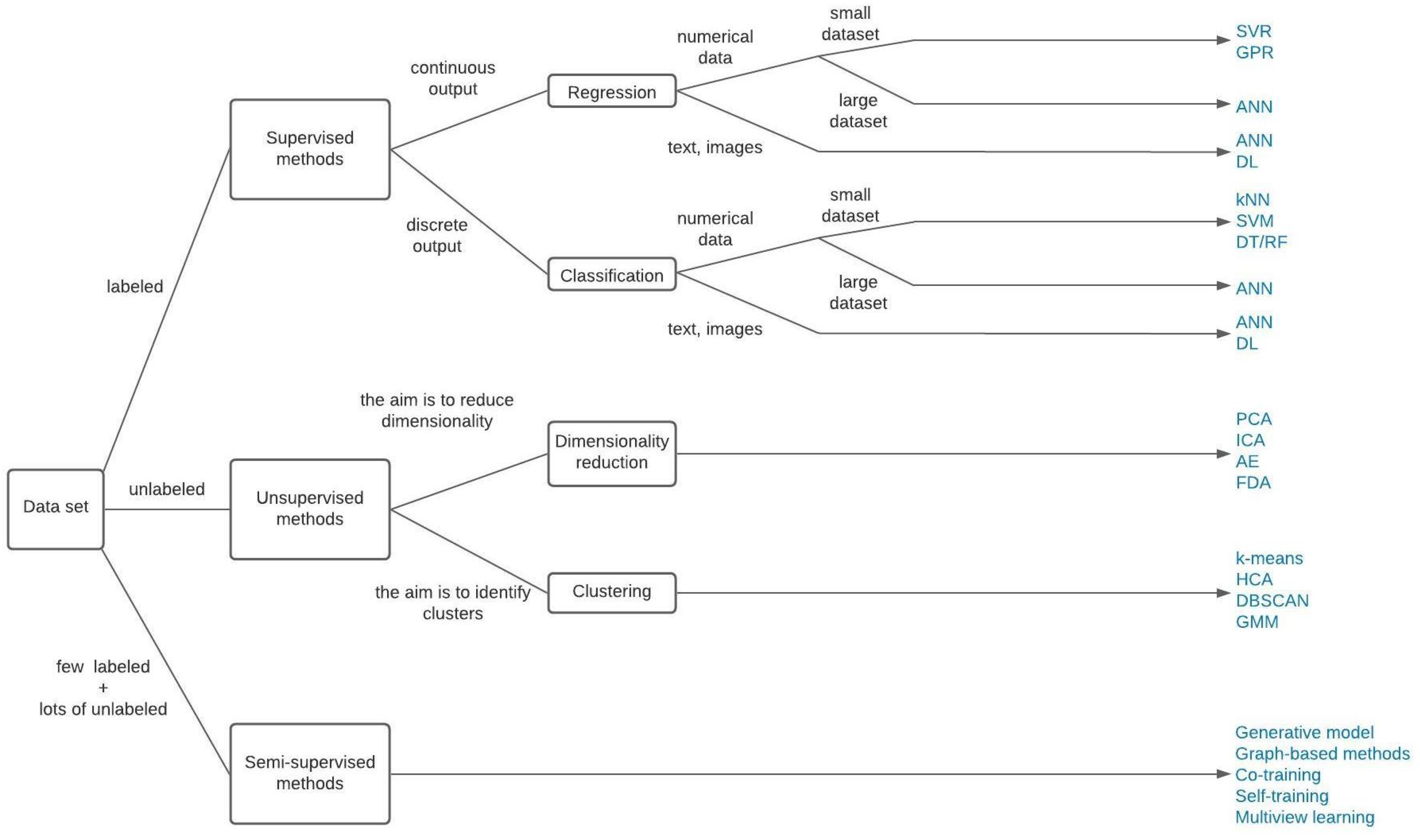
4.4. General Guidelines for the Selection of a ML Method

Unfortunately, a clear recipe or guide for the selection of the appropriate ML method for a given application does not exist. However, on the basis of the aforementioned characteristics and limitations of the different techniques, it is possible to distill a number of general good-practice rules that may serve as initial guidelines throughout this selection process. These rules are by no means explicit or novel and should be considered in combination with the specific characteristics of the problem at hand.

The first thing to consider is the necessity and interest in the implementation of a ML method with respect to alternative knowledge-based or different data-driven approaches according to the discussion presented in Section 4.2. Once the objectives of the study have been clarified and the implementation of a ML technique has been identified as an interesting approach, there are several other factors that need to be considered before homing in on a specific technique. Note that, whenever phenomenological models are available, hybrid modeling approaches should be pursued.

As ML methods are data-driven methods, the characteristics of data, such as their type (i.e., labeled or unlabeled), their amount and their structure (i.e., text, table, molecules etc.) will greatly influence this choice. As such, if the data is labeled or not will determine whether the selection should be directed toward a supervised or unsupervised learning method, respectively. In the intermediate case of the existence of both labeled and unlabeled data, semi-supervised methods should be preferred.

Furthermore, if the labels of the data are continuous values, a regression technique will be in order, while discrete labels will require the implementation of a classification technique. The structure of the data will also influence the choice toward certain types of methods. While all methods are generally compatible with numerical data (such as vectors and tables), ANN and especially DL methods will be more adapted to more complex data structures, such as texts and images.

The amount of data can also be used to facilitate the selection of the proper ML technique. As a general rule of thumb, it is considered that higher amounts of data are related to better ML model performance. This is especially true for ANN and DL, which require large data sets due to their increased number of parameters. A frequently asked question concerns the number of data necessary to consider a data set large enough for solving a problem.

Although there is no straightforward answer to this question, it should be taken into account that the necessity of large data sets is directly related to the complexity of the formulated model, which, in turn, is proportional to the complexity of the problem (including the complexity of the data). At the same time, it is important to remember that the above general rule of requirement of large data sets is not applicable to all ML techniques. In fact, as discussed previously, certain ML methods, such as SVM, GP, kNN and kmeans clustering, are rather more adapted to small data sets, which makes them excellent candidates for problems of limited data availability.

Several other aspects can also be considered for the selection of the appropriate learning algorithm, such as the sophistication level of the associated mathematical principles of the method, the training speed, the prediction speed and the non-linearity of the problem [31]. For example, concerning the first of these aspects, some ML methods are easier to use and to explain to a non-expert audience, such as kNN, linear regression and decision trees, in comparison to more sophisticated methods, like ANN, DL and SVM.

This can significantly increase their attractiveness toward occasional users or when the explanation of the implementation of the ML technique is part of the scope of the study (e.g., for educational purposes). The training speed can also be a decisive factor, in combination with the available computational resources. For example, the training of large ANNs of different structures, as part of the network architecture optimization, may require several hours, or even days, to accomplish.

In parallel to the selection of the ML method, another important decision that displays a direct effect on the performance of the developed model concerns the selection of the features. Ideally, all possible factors that may have an influence on the selected response should be included in the features list of the problem. However, since this information is rarely known a priori, there is a tendency to include as many features as possible in the training of the model in order to increase the possibility of capturing underlying relations and effects. This strategy may result in actually decreasing the capacity of the model to generalize its predictions, due to the so-called “overfitting” phenomenon, where the over accumulated noise in the data is “learned” by the model [194,197].

This problem is particularly intense with ANNs [30]. At the same time, the computational demands of the model increase along as well. To overcome this problem, the necessary amount of uncorrelated features can be selected on the basis of existing knowledge, whenever available, or by using dimensionality reduction methods, such as PCA or AE, prior to the learning step. Regularization or data partitioning into different data sets to be used for the model training, validation (i.e., to check the convergence of the training process or to tune some hyper-parameters of the model) and testing (i.e., to check the performance of the model on a fresh data set, once the training process has been concluded) are also efficient counter measures against overfitting.

Inversely, overlooking or omitting an important feature in the training process, in view of keeping the model simple and reducing the probability of overfitting, will impact the model performance as well since the model will be too simple to learn the underlying structure of data and/or incapable of identifying the complete relations between input and output, thereby, resulting in the opposite situation of underfitting. The above general guidelines are presented in the form of a decision tree in Figure 8.

5. Conclusions

Over the last decade, AI and ML techniques have been increasingly applied in CPE in order to solve the numerous complex challenges: the complexity of the structure-process–properties–ingredients interplay of the products and the necessity to quickly discover and constantly develop new molecules, materials, reactions and properties. In the present work, special emphasis was given to four selected domains, namely the design/discovery of new molecules/materials, the prediction of chemical reactions/retrosynthesis, the modeling of processes and the support for sensorial analysis.

Applications in the first two domains are relatively recent and intensive compared with the two others. The development of DL during the last decade enabled the tackling of extremely complex problems characterizing these first two domains, such as the exploration of the vast chemical space for both small organic compounds in the pharmaceutical industry and in materials.

More generally, the state of the art highlights the wide diversity in terms of the data characteristics among the different domains but also among the applications of a given domain. This provided a plethora of alternative ML approaches for the various problem types and data characteristics. Supervised, unsupervised and hybrid methods were found to be the most frequently implemented in CPE.

In addition, even if each domain displayed specific challenges, several common challenges could be identified, such as the ones related to data (i.e., data availability, data quality and chemical data representation), which are predominant in CPE as they are relatively more expensive and time-consuming to generate, with respect to other research domains. They are also rarely publicly available due to strong confidentiality and competitiveness limitations. This has lead to a significant growth in the use of ML methods that are specifically adapted to small data sets as well as to the development of massive data standardization and sharing initiatives.

Finally, even though a precise guide indicating the optimal ML method to use for a given problem does not exist, some guidelines are still provided here based on the problem constraints as well as on the characteristics of the available data.

References

1. Mitchell, T. Machine Learning; McGraw-Hill: New York, NY, USA, 1997. [Google Scholar]
2. Butler, K.T.; Davies, D.W.; Cartwright, H.; Isayev, O.; Walsh, A. Machine learning for molecular and materials science. Nature 2018, 559, 547–555. [Google Scholar] [CrossRef] [PubMed]
3. Elton, D.C.; Boukouvalas, Z.; Fuge, M.D.; Chung, P.W. Deep learning for molecular design-A review of the state of the art. Mol. Syst. Des. Eng. 2019, 4, 828–849. [Google Scholar] [CrossRef] [Green Version]
4. Pilania, G. Machine learning in materials science: From explainable predictions to autonomous design. Comput. Mater. Sci. 2021, 193, 110360. [Google Scholar] [CrossRef]
5. Zhou, T.; Song, Z.; Sundmacher, K. Big Data Creates New Opportunities for Materials Research: A Review on Methods and Applications of Machine Learning for Materials Design. Engineering 2019, 5, 1017–1026. [Google Scholar] [CrossRef]
6. Schmidt, J.; Marques, M.R.; Botti, S.; Marques, M.A. Recent advances and applications of machine learning in solid-state materials science. NPJ Comput. Mater. 2019, 5, 1–36. [Google Scholar] [CrossRef]
7. Westermayr, J.; Gastegger, M.; Schütt, K.T.; Maurer, R.J. Deep integration of machine learning into computational chemistry and materials science. arXiv 2021, arXiv:2102.08435v1. [Google Scholar]
8. Himanen, L.; Geurts, A.; Foster, A.S.; Rinke, P. Data-Driven Materials Science: Status, Challenges, and Perspectives. Adv. Sci. 2019, 6, 1900808. [Google Scholar] [CrossRef] [PubMed]
9. Winkler, D.A. Chapter 9 Machine Learning at the (Nano)materials-biology Interface. In Machine Learning in Chemistry: The Impact of Artificial Intelligence; The Royal Society of Chemistry: London, UK, 2020; pp. 206–226. [Google Scholar] [CrossRef]
10. Bennett, S.; Tarzia, A.; Zwijnenburg, M.A.; Jelfs, K.E. Chapter 12 Artificial Intelligence Applied to the Prediction of Organic Materials. In Machine Learning in Chemistry: The Impact of Artificial Intelligence; The Royal Society of Chemistry: London, UK, 2020; pp. 280–310. [Google Scholar] [CrossRef]
11. Zhuo, Y.; Tehrani, A.M.; Brgoch, J. Chapter 13 A New Era of Inorganic Materials Discovery Powered by Data Science. In Machine Learning in Chemistry: The Impact of Artificial Intelligence; The Royal Society of Chemistry: London, UK, 2020; pp. 311–339. [Google Scholar] [CrossRef]
12. Ramprasad, R.; Batra, R.; Mannodi-Kanakkithodi, A.; Kim, C.; Pilania, G. Machine learning in materials informatics: Recent applications and prospects. NPJ Comput. Mater. 2017, 3, 54. [Google Scholar] [CrossRef]
13. Chen, A.; Zhang, X.; Zhou, Z. Machine learning: Accelerating materials development for energy storage and conversion. InfoMat 2020, 2, 553–576. [Google Scholar] [CrossRef]
14. Zhu, H. Big data and artificial intelligence modeling for drug discovery. Annu. Rev. Pharmacol. Toxicol. 2020, 60, 573–589. [Google Scholar] [CrossRef] [PubMed] [Green Version]
15. Yang, X.; Wang, Y.; Byrne, R.; Schneider, G.; Yang, S. Concepts of Artificial Intelligence for Computer-Assisted Drug Discovery. Chem. Rev. 2019, 119, 10520–10594. [Google Scholar] [CrossRef] [PubMed] [Green Version]
16. Lo, Y.C.; Ren, G.; Honda, H.; Davis, K.L. Artificial Intelligence-Based Drug Design and Discovery; Intech: London, UK, 2019. [Google Scholar] [CrossRef] [Green Version]
17. Brown, N.; Ertl, P.; Lewis, R.; Luksch, T.; Reker, D.; Schneider, N. Artificial Intelligence in Chemistry and Drug Design; Springer Nature Swirzerland AG: Cham, Swirzerland, 2020. [Google Scholar] [CrossRef]
18. Klambauer, G.; Hochreiter, S.; Rarey, M. Machine Learning in Drug Discovery. J. Chem. Inf. Model. 2019, 59, 945–946. [Google Scholar] [CrossRef] [PubMed] [Green Version]
19. Schlexer Lamoureux, P.; Winther, K.T.; Garrido Torres, J.A.; Streibel, V.; Zhao, M.; Bajdich, M.; Abild-Pedersen, F.; Bligaard, T. Machine Learning for Computational Heterogeneous Catalysis. ChemCatChem 2019, 11, 3581–3601. [Google Scholar] [CrossRef] [Green Version]
20. Ma, S.; Kang, P.L.; Shang, C.; Liu, Z.P. Chapter 19 Machine Learning for Heterogeneous Catalysis: Global Neural Network Potential from Construction to Applications. In Machine Learning in Chemistry: The Impact of Artificial Intelligence; The Royal Society of Chemistry: London, UK, 2020; pp. 488–511. [Google Scholar] [CrossRef]
21. Yang, W.; Fidelis, T.T.; Sun, W.H. Machine Learning in Catalysis, From Proposal to Practicing. ACS Omega 2020, 5, 83–88. [Google Scholar] [CrossRef] [PubMed] [Green Version]
22. Nair, V.H.; Schwaller, P.; Laino, T. Data-driven Chemical Reaction Prediction and Retrosynthesis. Chimia 2019, 73, 997–1000. [Google Scholar] [CrossRef] [PubMed]
23. Coley, C.W.; Green, W.H.; Jensen, K.F. Machine Learning in Computer-Aided Synthesis Planning. Acc. Chem. Res. 2018, 51, 1281–1289. [Google Scholar] [CrossRef] [PubMed]
24. Haywood, A.L.; Redshaw, J.; Gaertner, T.; Taylor, A.; Mason, A.M.; Hirst, J.D. Chapter 7 Machine Learning for Chemical Synthesis. In Machine Learning in Chemistry: The Impact of Artificial Intelligence; The Royal Society of Chemistry: London, UK, 2020; pp. 169–194. [Google Scholar] [CrossRef]
25. Commenge, J.M. Big Data et Intelligence Artificielle pour le Génie des Procédés 2021. Available online: https://hal.univ-lorraine.fr/hal-03107557/document (accessed on 10 August 2021).
26. Ge, Z.; Song, Z.; Ding, S.X.; Huang, B. Data Mining and Analytics in the Process Industry: The Role of Machine Learning. IEEE Access 2017, 5, 20590–20616. [Google Scholar] [CrossRef]
27. Yan, Y.; Borhani, T.N.; Clough, P.T. Chapter 14 Machine Learning Applications in Chemical Engineering. In Machine Learning in Chemistry: The Impact of Artificial Intelligence; The Royal Society of Chemistry: London, UK, 2020; pp. 340–371. [Google Scholar] [CrossRef]
28. Wang, C.; Tan, X.P.; Tor, S.B.; Lim, C.S. Machine learning in additive manufacturing: State-of-the-art and perspectives. Addit. Manuf. 2020, 36, 101538. [Google Scholar] [CrossRef]
29. DebRoy, T.; Mukherjee, T.; Wei, H.L.; Elmer, J.W.; Milewski, J.O. Metallurgy, mechanistic models and machine learning in metal printing. Nat. Rev. Mater. 2021, 6, 48–68. [Google Scholar] [CrossRef]
30. Géron, A. Hands-on Machine Learning with Scikit-Learn, Keras, and TensorFlow: Concepts, Tools, and Techniques to Build Intelligent Systems; O’Reilly Media, Inc.: Sebastopol, CA, USA, 2019. [Google Scholar]
31. Burkov, A. The Hundred-Page Machine Learning Book; Andriy Burkov: Quebec City, QC, Canada, 2019. [Google Scholar]
32. Nasery, S.; Hoseinpour, S.; Phung, L.T.K.; Bahadori, A. Prediction of the viscosity of water-in-oil emulsions. Pet. Sci. Technol. 2016, 34, 1972–1977. [Google Scholar] [CrossRef]
33. Gola, J.; Webel, J.; Britz, D.; Guitar, A.; Staudt, T.; Winter, M.; Mücklich, F. Objective microstructure classification by support vector machine (SVM) using a combination of morphological parameters and textural features for low carbon steels. Comput. Mater. Sci. 2019, 160, 186–196. [Google Scholar] [CrossRef]
34. Zhu, H.; Liu, F.; Ye, Y.; Chen, L.; Liu, J.; Gui, A.; Zhang, J.; Dong, C. Application of machine learning algorithms in quality assurance of fermentation process of black tea— based on electrical properties. J. Food Eng. 2019, 263, 165–172. [Google Scholar] [CrossRef]
35. Ge, Z.; Chen, T.; Song, Z. Quality prediction for polypropylene production process based on CLGPR model. Control. Eng. Pract. 2011, 19, 423–432. [Google Scholar] [CrossRef] [Green Version]
36. Zheng, W.; Gao, X.; Liu, Y.; Wang, L.; Yang, J.; Gao, Z. Industrial Mooney viscosity prediction using fast semi-supervised empirical model. Chemom. Intell. Lab. Syst. 2017, 171, 86–92. [Google Scholar] [CrossRef]
37. Liang, Y.; Liu, Z.; Liu, W. A co-training style semi-supervised artificial neural network modeling and its application in thermal conductivity prediction of polymeric composites filled with BN sheets. Energy AI 2021, 4, 100052. [Google Scholar] [CrossRef]
38. Yan, W.; Guo, P.; Tian, Y.; Gao, J. A Framework and Modeling Method of Data-Driven Soft Sensors Based on Semisupervised Gaussian Regression. Ind. Eng. Chem. Res. 2016, 55, 7394–7401. [Google Scholar] [CrossRef]
39. Liu, Y.; Yang, C.; Gao, Z.; Yao, Y. Ensemble deep kernel learning with application to quality prediction in industrial polymerization processes. Chemom. Intell. Lab. Syst. 2018, 174, 15–21. [Google Scholar] [CrossRef]
40. Yin, X.; Niu, Z.; He, Z.; Li, Z.; hee Lee, D. Ensemble deep learning based semi-supervised soft sensor modeling method and its application on quality prediction for coal preparation process. Adv. Eng. Inform. 2020, 46, 101136. [Google Scholar] [CrossRef]
41. He, X.; Ji, J.; Liu, K.; Gao, Z.; Liu, Y. Soft sensing of silicon content via bagging local semi-supervised models. Sensors 2019, 19, 3814. [Google Scholar] [CrossRef] [Green Version]
42. Ma, W.; Cheng, F.; Xu, Y.; Wen, Q.; Liu, Y. Probabilistic Representation and Inverse Design of Metamaterials Based on a Deep Generative Model with Semi-Supervised Learning Strategy. Adv. Mater. 2019, 31, 1–9. [Google Scholar] [CrossRef] [PubMed] [Green Version]
43. Okaro, I.A.; Jayasinghe, S.; Sutcliffe, C.; Black, K.; Paoletti, P.; Green, P.L. Automatic fault detection for laser powder-bed fusion using semi-supervised machine learning. Addit. Manuf. 2019, 27, 42–53. [Google Scholar] [CrossRef]
44. Zhang, Y.; Lu, Z. Exploring semi-supervised variational autoencoders for biomedical relation extraction. Methods 2019, 166, 112–119. [Google Scholar] [CrossRef] [Green Version]
45. Sahoo, P.; Roy, I.; Wang, Z.; Mi, F.; Yu, L.; Balasubramani, P.; Khan, L.; Stoddart, J.F. MultiCon: A Semi-Supervised Approach for Predicting Drug Function from Chemical Structure Analysis. J. Chem. Inf. Model. 2020, 60, 5995–6006. [Google Scholar] [CrossRef] [PubMed]
46. Yu, H.; Ji, J.; Li, P.; Shao, F.; Wu, S.; Sui, Y.; Li, S.; He, F.; Liu, J. Semi-Supervised Hybrid Local Kernel Regression for Soft Sensor Modelling of Rubber-Mixing Process. Adv. Polym. Technol. 2020, 2020, 6981302. [Google Scholar] [CrossRef]
47. Zheng, J.; Du, J.; Liang, Y.; Liao, Q.; Li, Z.; Zhang, H.; Wu, Y. Deeppipe: A semi-supervised learning for operating condition recognition of multi-product pipelines. Process. Saf. Environ. Prot. 2021, 150, 510–521. [Google Scholar] [CrossRef]
48. Ma, Y.; Zhu, W.; Benton, M.; Romagnoli, J. Continuous control of a polymerization system with deep reinforcement learning. J. Process. Control. 2019, 75, 40–47. [Google Scholar] [CrossRef]
49. Singh, V.; Kodamana, H. Reinforcement learning based control of batch polymerisation processes. IFAC PapersOnLine 2020, 53, 667–672. [Google Scholar] [CrossRef]
50. Nian, R.; Liu, J.; Huang, B. A review On reinforcement learning: Introduction and applications in industrial process control. Comput. Chem. Eng. 2020, 139, 106886. [Google Scholar] [CrossRef]
51. Venkatasubramanian, V. The promise of artificial intelligence in chemical engineering: Is it here, finally? AIChE J. 2019, 65, 466–478. [Google Scholar] [CrossRef]
52. Zendehboudi, S.; Rezaei, N.; Lohi, A. Applications of hybrid models in chemical, petroleum, and energy systems: A systematic review. Appl. Energy 2018, 228, 2539–2566. [Google Scholar] [CrossRef]
53. Uhlemann, J.; Costa, R. Product Design and Engineering in Chemical Engineering: Past, Present State, and Future. Chem. Eng. Technol. 2019, 42, 2258–2274. [Google Scholar] [CrossRef]
54. Meng, Y.; Yu, S.; Zhang, J.; Qin, J.; Dong, Z.; Lu, G. Hybrid modeling based on mechanistic and data-driven approaches for cane sugar crystallization. J. Food Eng. 2019, 257, 44–55. [Google Scholar] [CrossRef]
55. Li, B.; Lin, Y.; Yu, W.; Wilson, D.I.; Young, B.R. Application of mechanistic modelling and machine learning for cream cheese fermentation pH prediction. J. Chem. Technol. Biotechnol. 2021, 96, 125–133. [Google Scholar] [CrossRef]
56. Zhang, X.; Zhou, T.; Zhang, L.; Fung, K.Y.; Ng, K.M. Food Product Design: A Hybrid Machine Learning and Mechanistic Modeling Approach. Ind. Eng. Chem. Res. 2019, 58, 16743–16752. [Google Scholar] [CrossRef]
57. von Stosch, M.; Davy, S.; Francois, K.; Galvanauskas, V.; Hamelink, J.M.; Luebbert, A.; Mayer, M.; Oliveira, R.; O’Kennedy, R.; Rice, P.; et al. Hybrid modeling for quality by design and PAT-benefits and challenges of applications in biopharmaceutical industry. Biotechnol. J. 2014, 9, 719–726. [Google Scholar] [CrossRef] [Green Version]
58. Drăgoi, E.N.; Curteanu, S.; Fissore, D.; Curteanu, S.; Fissore, D. On the Use of Artificial Neural Networks to Monitor a Pharmaceutical Freeze-Drying Process On the Use of Artificial Neural Networks to Monitor a Pharmaceutical Freeze-Drying Process. Dry. Technol. 2013, 31, 72–81. [Google Scholar] [CrossRef] [Green Version]
59. Calvo, F.; Gómez, J.M.; Ricardez-Sandoval, L.; Alvarez, O. Integrated design of emulsified cosmetic products: A review. Chem. Eng. Res. Des. 2020, 161, 279–303. [Google Scholar] [CrossRef]
60. Sadowski, P.; Fooshee, D.; Subrahmanya, N.; Baldi, P. Synergies between quantum mechanics and machine learning in reaction prediction. J. Chem. Inf. Model. 2016, 56, 2125–2128. [Google Scholar] [CrossRef]
61. Castéran, F.; Ibanez, R.; Argerich, C.; Delage, K.; Chinesta, F.; Cassagnau, P. Application of Machine Learning Tools for the Improvement of Reactive Extrusion Simulation. Macromol. Mater. Eng. 2020, 305, 2000375. [Google Scholar] [CrossRef]
62. Ghiba, L.; Drăgoi, E.N.; Curteanu, S. Neural network-based hybrid models developed for free radical polymerization of styrene. Polym. Eng. Sci. 2021, 61, 716–730. [Google Scholar] [CrossRef]
63. Curteanu, S.; Leon, F. Hybrid neural network models applied to a free radical polymerization process. Polym. Plast. Technol. Eng. 2006, 45, 1013–1023. [Google Scholar] [CrossRef]
64. Ng, C.W.; Hussain, M.A. Hybrid neural network-prior knowledge model in temperature control of a semi-batch polymerization process. Chem. Eng. Process. Process. Intensif. 2004, 43, 559–570. [Google Scholar] [CrossRef]
65. Qi, C.; Ly, H.B.; Chen, Q.; Le, T.T.; Le, V.M.; Pham, B.T. Flocculation-dewatering prediction of fine mineral tailings using a hybrid machine learning approach. Chemosphere 2020, 244, 125450. [Google Scholar] [CrossRef]
66. Bi, K.; Qiu, T.; Huang, Y. A deep learning method for yogurt preferences prediction using sensory attributes. Processes 2020, 8, 518. [Google Scholar] [CrossRef]
67. Chen, L.; Kim, C.; Batra, R.; Lightstone, J.P.; Wu, C.; Li, Z.; Deshmukh, A.A.; Wang, Y.; Tran, H.D.; Vashishta, P.; et al. Frequency-dependent dielectric constant prediction of polymers using machine learning. NPJ Comput. Mater. 2020, 6, 30–32. [Google Scholar] [CrossRef]
68. Batra, R.; Dai, H.; Huan, T.D.; Chen, L.; Kim, C.; Gutekunst, W.R.; Song, L.; Ramprasad, R. Polymers for Extreme Conditions Designed Using Syntax-Directed Variational Autoencoders. Chem. Mater. 2020, 32, 10489–10500. [Google Scholar] [CrossRef]
69. Zhou, T.; Gani, R.; Sundmacher, K. Hybrid data-driven and mechanistic modeling approaches for multiscale material and process design. Engineering 2021. [Google Scholar] [CrossRef]
70. McBride, K.; Sanchez Medina, E.I.; Sundmacher, K. Hybrid Semi-parametric Modeling in Separation Processes: A Review. Chem. Ingenieur-Technik 2020, 92, 842–855. [Google Scholar] [CrossRef]
71. Zhang, X.; Ding, X.; Song, Z.; Zhou, T.; Sundmacher, K. Integrated ionic liquid and rate-based absorption process design for gas separation: Global optimization using hybrid models. AIChE J. 2021, e17340. [Google Scholar] [CrossRef]
72. Zhang, L.; Mao, H.; Liu, Q.; Gani, R. Chemical product design–recent advances and perspectives. Curr. Opin. Chem. Eng. 2020, 27, 22–34. [Google Scholar] [CrossRef]
73. Costa, R.; Moggridge, G.D.; Saraiva, P.M. Chemical Product Engineering: An Emerging Paradigm within Chemical Engineering. Aiche J. 2006, 52, 1976–1986. [Google Scholar] [CrossRef] [Green Version]
74. Arrieta-Escobar, J.A.; Camargo, M.; Morel, L.; Orjuela, A. Current approaches on chemical product design: A study of opportunities identification for integrated methodologies. In Proceedings of the Towards the Digital World and Industry X.0-Proceedings of the 29th International Conference of the International Association for Management of Technology, IAMOT 2020, Cairo, Egypt, 13–17 September 2020; pp. 785–794. [Google Scholar]
75. Ng, K.M.; Gani, R. Chemical product design: Advances in and proposed directions for research and teaching. Comput. Chem. Eng. 2019, 126, 147–156. [Google Scholar] [CrossRef]
76. Cussler, E.L. Chemical Product Design; Cambridge University Press: Cambridge, UK; New York, NY, USA, 2011. [Google Scholar]
77. Hill, M. Chemical Product Engineering-The third paradigm. Comput. Chem. Eng. 2009, 33, 947–953. [Google Scholar] [CrossRef]
78. Taifouris, M.; Martín, M.; Martínez, A.; Esquejo, N. Challenges in the design of formulated products: Multiscale process and product design. Curr. Opin. Chem. Eng. 2020, 27, 1–9. [Google Scholar] [CrossRef]
79. Fischer, A. Artificial Intelligence Colloquium: Accelerating Chemistry with AI. 2019. Available online: https://theengineeringofconsciousexperience.com/artificial-intelligence-colloquium-accelerating-chemistry-with-ai/ (accessed on 10 August 2021).
80. Goussard, V.; Duprat, F.; Ploix, J.L.; Dreyfus, G.; Nardello-Rataj, V.; Aubry, J.M. A New Machine-Learning Tool for Fast Estimation of Liquid Viscosity. Application to Cosmetic Oils. J. Chem. Inf. Model. 2020, 60, 2012–2023. [Google Scholar] [CrossRef]
81. Dobbelaere, M.R.; Plehiers, P.P.; Van de Vijver, R.; Stevens, C.V.; Van Geem, K.M. Learning Molecular Representations for Thermochemistry Prediction of Cyclic Hydrocarbons and Oxygenates. J. Phys. Chem. A 2021, 125, 5166–5179. [Google Scholar] [CrossRef]
82. Lo, Y.C.; Rensi, S.E.; Torng, W.; Altman, R.B. Machine learning in chemoinformatics and drug discovery. Drug Discov. Today 2018, 23, 1538–1546. [Google Scholar] [CrossRef] [PubMed]
83. Smith, J.S.; Roitberg, A.E.; Isayev, O. Transforming Computational Drug Discovery with Machine Learning and AI. ACS Med. Chem. Lett. 2018, 9, 1065–1069. [Google Scholar] [CrossRef] [PubMed]
84. David, L.; Thakkar, A.; Mercado, R.; Engkvist, O. Molecular representations in AI-driven drug discovery: A review and practical guide. J. Cheminform. 2020, 12, 56. [Google Scholar] [CrossRef] [PubMed]
85. Sanchez-Lengeling, B.; Aspuru-Guzik, A. Inverse molecular design using machine learning: Generative models for matter engineering. Science 2018, 361, 360–365. [Google Scholar] [CrossRef] [Green Version]
86. Staker, J.; Marques, G.; Dakka, J. Chapter 15 Representation Learning in Chemistry. In Machine Learning in Chemistry: The Impact of Artificial Intelligence; The Royal Society of Chemistry: London, UK, 2020; pp. 372–397. [Google Scholar] [CrossRef]
87. Alshehri, A.S.; Gani, R.; You, F. Deep learning and knowle dge-base d methods for computer-aided molecular design—Toward a unified approach: State-of-the-art and future directions. Comput. Chem. Eng. 2020, 141, 107005. [Google Scholar] [CrossRef]
88. Audus, D.J.; De Pablo, J.J. Polymer Informatics: Opportunities and Challenges. ACS Macro Lett. 2017, 6, 1078–1082. [Google Scholar] [CrossRef]
89. Wei, J.N. Exploring Machine Learning Applications to Enable Next-Generation Chemistry. Ph.D. Thesis, Harvard University, Cambridge, MA, USA, 2019. [Google Scholar]
90. Luan, F. Classification of the fragrance properties of chemical compounds based on support vector machine and linear discriminant analysis. Flavour Fragr. J. 2007, 23, 311–316. [Google Scholar] [CrossRef]
91. Kennedy, K.; Cal, R.; Casey, R.; Lopez, C.; Adelfio, A.; Molloy, B.; Wall, A.M.; Holton, T.A.; Khaldi, N. The anti-ageing effects of a natural peptide discovered by artificial intelligence. Int. J. Cosmet. Sci. 2020, 42, 388–398. [Google Scholar] [CrossRef]
92. Lightstone, J.P.; Chen, L.; Kim, C.; Batra, R.; Ramprasad, R. Refractive index prediction models for polymers using machine learning. J. Appl. Phys. 2020, 127, 215105. [Google Scholar] [CrossRef]
93. Zhang, Y.; Xu, X. Machine learning glass transition temperature of polymers. Heliyon 2020, 6, e05055. [Google Scholar] [CrossRef]
94. Yang, Y.; Zhang, X.; Yin, J.; Yu, X. Rapid and Nondestructive On-Site Classification Method for Consumer-Grade Plastics Based on Portable NIR Spectrometer and Machine Learning. J. Spectrosc. 2020, 2020, 6631234. [Google Scholar] [CrossRef]
95. Bieler, M.; Reutlinger, M.; Rodrigues, T.; Schneider, P.; Kriegl, J.M.; Schneider, G. Designing Multi-target Compound Libraries with Gaussian Process Models. Mol. Inform. 2016, 35, 192–198. [Google Scholar] [CrossRef] [PubMed] [Green Version]
96. Zhu, G.; Kim, C.; Chandrasekarn, A.; Everett, J.; Ramprasad, R.; Lively, R.P. Polymer genome-based prediction of gas permeabilities in polymers. J. Polym. Eng. 2020, 40, 451–457. [Google Scholar] [CrossRef]
97. Song, Z.; Shi, H.; Zhang, X.; Zhou, T. Prediction of CO2 solubility in ionic liquids using machine learning methods. Chem. Eng. Sci. 2020, 223, 115752. [Google Scholar] [CrossRef]
98. Doan Tran, H.; Kim, C.; Chen, L.; Chandrasekaran, A.; Batra, R.; Venkatram, S.; Kamal, D.; Lightstone, J.P.; Gurnani, R.; Shetty, P.; et al. Machine-learning predictions of polymer properties with Polymer Genome. J. Appl. Phys. 2020, 128, 171104. [Google Scholar] [CrossRef]
99. Zhang, X.; Wang, J.; Song, Z.; Zhou, T. Data-Driven Ionic Liquid Design for CO2 Capture: Molecular Structure Optimization and DFT Veri fi cation. Ind. Eng. Chem. Res. 2021, 60, 9992–10000. [Google Scholar] [CrossRef]
100. Haghighatlari, M.; Hachmann, J. Advances of machine learning in molecular modeling and simulation. Curr. Opin. Chem. Eng. 2019, 23, 51–57. [Google Scholar] [CrossRef] [Green Version]
101. Pilania, G.; Wang, C.; Jiang, X.; Rajasekaran, S.; Ramprasad, R. Accelerating materials property predictions using machine learning. Sci. Rep. 2013, 3, 2810. [Google Scholar] [CrossRef]
102. Yeo, C.S.H.; Xie, Q.; Wang, X.; Zhang, S. Understanding and optimization of thin film nanocomposite membranes for reverse osmosis with machine learning. J. Membr. Sci. 2020, 606, 118135. [Google Scholar] [CrossRef]
103. Yan, Y.; Mattisson, T.; Moldenhauer, P.; Anthony, E.J.; Clough, P.T. Applying machine learning algorithms in estimating the performance of heterogeneous, multi-component materials as oxygen carriers for chemical-looping processes. Chem. Eng. J. 2020, 387, 124072. [Google Scholar] [CrossRef]
104. Sun, Y.; Hewitt, M.; Wilkinson, S.C.; Davey, N.; Adams, R.G.; Gullick, D.R.; Moss, G.P. Development of a Gaussian Process–feature selection model to characterise (poly)dimethylsiloxane (Silastic®) membrane permeation. J. Pharm. Pharmacol. 2020, 72, 873–888. [Google Scholar] [CrossRef] [Green Version]
105. Ju, S.; Shimizu, S.; Shiomi, J. Designing thermal functional materials by coupling thermal transport calculations and machine learning. J. Appl. Phys. 2020, 128, 161102. [Google Scholar] [CrossRef]
106. Jiao, P.; Alavi, A.H. Artificial intelligence-enabled smart mechanical metamaterials: Advent and future trends. Int. Mater. Rev. 2021, 66, 365–393. [Google Scholar] [CrossRef]
107. Chen, C.; Zuo, Y.; Ye, W.; Li, X.; Deng, Z.; Ong, S.P. A Critical Review of Machine Learning of Energy Materials. Adv. Energy Mater. 2020, 10, 1903242. [Google Scholar] [CrossRef]
108. Christensen, T.; Loh, C.; Picek, S.; Jakobović, D.; Jing, L.; Fisher, S.; Ceperic, V.; Joannopoulos, J.D.; Soljačić, M. Predictive and generative machine learning models for photonic crystals. Nanophotonics 2020, 9, 4183–4192. [Google Scholar] [CrossRef]
109. Xie, Y.; Zhang, C.; Hu, X.; Zhang, C.; Kelley, S.P.; Atwood, J.L.; Lin, J. Machine Learning Assisted Synthesis of Metal-Organic Nanocapsules. J. Am. Chem. Soc. 2020, 142, 1475–1481. [Google Scholar] [CrossRef] [Green Version]
110. Li, F.; Han, J.; Cao, T.; Lam, W.; Fan, B.; Tang, W.; Chen, S.; Fok, K.L.; Li, L. Design of self-assembly dipeptide hydrogels and machine learning via their chemical features. Proc. Natl. Acad. Sci. USA 2019, 166, 11259–11264. [Google Scholar] [CrossRef] [Green Version]
111. Gu, G.H.; Noh, J.; Kim, I.; Jung, Y. Machine learning for renewable energy materials. J. Mater. Chem. A 2019, 7, 17096–17117. [Google Scholar] [CrossRef]
112. Conduit, B.D.; Illston, T.; Baker, S.; Duggappa, D.V.; Harding, S.; Stone, H.J.; Conduit, G.J. Probabilistic neural network identification of an alloy for direct laser deposition. Mater. Des. 2019, 168, 107644. [Google Scholar] [CrossRef]
113. Balachandran, P.V. Machine learning guided design of functional materials with targeted properties. Comput. Mater. Sci. 2019, 164, 82–90. [Google Scholar] [CrossRef]
114. Noack, M.M.; Doerk, G.S.; Li, R.; Streit, J.K.; Vaia, R.A.; Yager, K.G.; Fukuto, M. Autonomous materials discovery driven by Gaussian process regression with inhomogeneous measurement noise and anisotropic kernels. Sci. Rep. 2020, 10, 17663. [Google Scholar] [CrossRef]
115. Mansouri Tehrani, A.; Oliynyk, A.O.; Parry, M.; Rizvi, Z.; Couper, S.; Lin, F.; Miyagi, L.; Sparks, T.D.; Brgoch, J. Machine Learning Directed Search for Ultraincompressible, Superhard Materials. J. Am. Chem. Soc. 2018, 140, 9844–9853. [Google Scholar] [CrossRef]
116. Tabor, D.P.; Roch, L.M.; Saikin, S.K.; Kreisbeck, C.; Sheberla, D.; Montoya, J.H.; Dwaraknath, S.; Aykol, M.; Ortiz, C.; Tribukait, H.; et al. Accelerating the discovery of materials for clean energy in the era of smart automation. Nat. Rev. Mater. 2018, 3, 5–20. [Google Scholar] [CrossRef] [Green Version]
117. Saeki, A. Evaluation-oriented exploration of photo energy conversion systems: From fundamental optoelectronics and material screening to the combination with data science. Polym. J. 2020, 52, 1307–1321. [Google Scholar] [CrossRef]
118. Kayala, M.A.; Baldi, P. ReactionPredictor: Prediction of complex chemical reactions at the mechanistic level using machine learning. J. Chem. Inf. Model. 2012, 52, 2526–2540. [Google Scholar] [CrossRef] [PubMed]
119. Schwaller, P.; Gaudin, T.; Lányi, D.; Bekas, C.; Laino, T. “Found in Translation”: Predicting outcomes of complex organic chemistry reactions using neural sequence-to-sequence models. Chem. Sci. 2018, 9, 6091–6098. [Google Scholar] [CrossRef] [Green Version]
120. Kayala, M.A.; Azencott, C.A.; Chen, J.H.; Baldi, P. Learning to predict chemical reactions. J. Chem. Inf. Model. 2011, 51, 2209–2222. [Google Scholar] [CrossRef] [Green Version]
121. Coley, C.W.; Barzilay, R.; Jaakkola, T.S.; Green, W.H.; Jensen, K.F. Prediction of Organic Reaction Outcomes Using Machine Learning. ACS Cent. Sci. 2017, 3, 434–443. [Google Scholar] [CrossRef] [PubMed] [Green Version]
122. Segler, M.H.; Waller, M.P. Neural-Symbolic Machine Learning for Retrosynthesis and Reaction Prediction. Chem. Eur. J. 2017, 23, 5966–5971. [Google Scholar] [CrossRef]
123. Segler, M.H.; Waller, M.P. Modelling Chemical Reasoning to Predict and Invent Reactions. Chem. Eur. J. 2017, 23, 6118–6128. [Google Scholar] [CrossRef] [PubMed] [Green Version]
124. Segler, M.H.; Preuss, M.; Waller, M.P. Planning chemical syntheses with deep neural networks and symbolic AI. Nature 2018, 555, 604–610. [Google Scholar] [CrossRef] [Green Version]
125. Schwaller, P.; Laino, T.; Gaudin, T.; Bolgar, P.; Hunter, C.A.; Bekas, C.; Lee, A.A. Molecular Transformer: A Model for Uncertainty-Calibrated Chemical Reaction Prediction. ACS Cent. Sci. 2019, 5, 1572–1583. [Google Scholar] [CrossRef] [Green Version]
126. Schwaller, P.; Petraglia, R.; Zullo, V.; Nair, V.H.; Haeuselmann, R.A.; Pisoni, R.; Bekas, C.; Iuliano, A.; Laino, T. Predicting retrosynthetic pathways using transformer-based models and a hyper-graph exploration strategy. Chem. Sci. 2020, 11, 3316–3325. [Google Scholar] [CrossRef] [Green Version]
127. Schwaller, P.; Hoover, B.; Reymond, J.L.; Strobelt, H.; Laino, T. Extraction of organic chemistry grammar from unsupervised learning of chemical reactions. Sci. Adv. 2021, 7, eabe4166. [Google Scholar] [CrossRef]
128. Gao, H.; Struble, T.J.; Coley, C.W.; Wang, Y.; Green, W.H.; Jensen, K.F. Using Machine Learning to Predict Suitable Conditions for Organic Reactions. ACS Cent. Sci. 2018, 4, 1465–1476. [Google Scholar] [CrossRef] [Green Version]
129. Wei, J.N.; Duvenaud, D.; Aspuru-Guzik, A. Neural networks for the prediction of organic chemistry reactions. ACS Cent. Sci. 2016, 2, 725–732. [Google Scholar] [CrossRef]
130. Ishida, S.; Terayama, K.; Kojima, R.; Takasu, K.; Okuno, Y. Prediction and Interpretable Visualization of Retrosynthetic Reactions Using Graph Convolutional Networks. J. Chem. Inf. Model. 2019, 59, 5026–5033. [Google Scholar] [CrossRef] [PubMed]
131. Nam, J.; Kim, J. Linking the Neural Machine Translation and the Prediction of Organic Chemistry Reactions. arXiv 2016, arXiv:1612.09529. [Google Scholar]
132. McCoy, J.T.; Auret, L. Machine learning applications in minerals processing: A review. Miner. Eng. 2019, 132, 95–109. [Google Scholar] [CrossRef]
133. Curteanu, S.; Leon, F.; Mircea-Vicoveanu, A.M.; Logofătu, D. Regression methods based on nearest neighbors with adaptive distance metrics applied to a polymerization process. Mathematics 2021, 9, 547. [Google Scholar] [CrossRef]
134. Curteanu, S. Chapter 10 Machine Learning Techniques Applied to a Complex Polymerization Process. In Machine Learning in Chemistry: The Impact of Artificial Intelligence; The Royal Society of Chemistry: London, UK, 2020; pp. 227–250. [Google Scholar] [CrossRef]
135. Meimaroglou, D.; Florez, D.; Hu, G.H. A kinetic modeling framework for the peroxide-initiated radical polymerization of styrene in the presence of rubber particles from recycled tires. Chem. Eng. Sci. 2020. under review. [Google Scholar]
136. Khayyam, H.; Jazar, R.N.; Nunna, S.; Golkarnarenji, G.; Badii, K.; Fakhrhoseini, S.M.; Kumar, S.; Naebe, M. PAN precursor fabrication, applications and thermal stabilization process in carbon fiber production: Experimental and mathematical modelling. Prog. Mater. Sci. 2020, 107, 100575. [Google Scholar] [CrossRef]
137. Kramer, A.; Morgado-Dias, F. Artificial intelligence in process control applications and energy saving: A review and outlook. Greenh. Gases Sci. Technol. 2020, 10, 1133–1150. [Google Scholar] [CrossRef]
138. Dong, E.L.; Song, J.H.; Song, S.O.; En, S.Y. Weighted support vector machine for quality estimation in the polymerization process. Ind. Eng. Chem. Res. 2005, 44, 2101–2105. [Google Scholar] [CrossRef]
139. Zhao, P.; Zhang, J.; Dong, Z.; Huang, J.; Zhou, H.; Fu, J.; Turng, L.S. Intelligent Injection Molding on Sensing, Optimization, and Control. Adv. Polym. Technol. 2020, 2020, 7023616. [Google Scholar] [CrossRef] [Green Version]
140. Khan, A.; Shamsi, M.H.; Choi, T.S. Correlating dynamical mechanical properties with temperature and clay composition of polymer-clay nanocomposites. Comput. Mater. Sci. 2009, 45, 257–265. [Google Scholar] [CrossRef]
141. Li, C.; Rubín De Celis Leal, D.; Rana, S.; Gupta, S.; Sutti, A.; Greenhill, S.; Slezak, T.; Height, M.; Venkatesh, S. Rapid Bayesian optimisation for synthesis of short polymer fiber materials. Sci. Rep. 2017, 7, 5683. [Google Scholar] [CrossRef]
142. Ibañez, R.; Casteran, F.; Argerich, C.; Ghnatios, C.; Hascoet, N.; Ammar, A.; Cassagnau, P.; Chinesta, F. On the data-driven modeling of reactive extrusion. Fluids 2020, 5, 94. [Google Scholar] [CrossRef]
143. Curteanu, S.; Leon, F.; Galea, D. Neural network models for free radical polymerization of methyl methacrylate Neural Network Models for Free Radical Polymerization of Methyl Methacrylate. Eurasian Chemtech. J. 2003, 5, 225–231. [Google Scholar]
144. Curteanu, S. Direct and inverse neural network modeling in free radical polymerization. Cent. Eur. J. Chem. 2004, 2, 113–140. [Google Scholar] [CrossRef]
145. Rodríguez-Dorado, R.; Landín, M.; Altai, A.; Russo, P.; Aquino, R.P.; Del Gaudio, P. A novel method for the production of core-shell microparticles by inverse gelation optimized with artificial intelligent tools. Int. J. Pharm. 2018, 538, 97–104. [Google Scholar] [CrossRef]
146. Rouco, H.; Diaz-Rodriguez, P.; Rama-Molinos, S.; Remuñán-López, C.; Landin, M. Delimiting the knowledge space and the design space of nanostructured lipid carriers through Artificial Intelligence tools. Int. J. Pharm. 2018, 553, 522–530. [Google Scholar] [CrossRef] [PubMed]
147. Wang, K.; Han, L.; Mustakis, J.; Li, B.; Magano, J.; Damon, D.B.; Dion, A.; Maloney, M.T.; Post, R.; Li, R. Kinetic and Data-Driven Reaction Analysis for Pharmaceutical Process Development. Ind. Eng. Chem. Res. 2020, 59, 2409–2421. [Google Scholar] [CrossRef]
148. Sarmadi, M.; Behrens, A.M.; McHugh, K.J.; Contreras, H.T.; Tochka, Z.L.; Lu, X.; Langer, R.; Jaklenec, A. Modeling, design, and machine learning-based framework for optimal injectability of microparticle-based drug formulations. Sci. Adv. 2020, 6, abb6594. [Google Scholar] [CrossRef]
149. Jhamb, S.; Enekvist, M.; Liang, X.; Zhang, X.; Dam-Johansen, K.; Kontogeorgis, G.M. A review of computer-aided design of paints and coatings. Curr. Opin. Chem. Eng. 2020, 27, 107–120. [Google Scholar] [CrossRef]
150. Jasso-Salcedo, A.B.; Hoppe, S.; Pla, F.; Escobar-Barrios, V.A.; Camargo, M.; Meimaroglou, D. Modeling and optimization of a photocatalytic process: Degradation of endocrine disruptor compounds by Ag/ZnO. Chem. Eng. Res. Des. 2017, 128, 174–191. [Google Scholar] [CrossRef]
151. Jeguirim, S.E.G.; Dhouib, A.B.; Sahnoun, M.; Cheikhrouhou, M.; Schacher, L.; Adolphe, D. The use of fuzzy logic and neural networks models for sensory properties prediction from process and structure parameters of knitted fabrics. J. Intell. Manuf. 2011, 22, 873–884. [Google Scholar] [CrossRef]
152. Golkarnarenji, G.; Naebe, M.; Badii, K.; Milani, A.S.; Jazar, R.N.; Khayyam, H. A machine learning case study with limited data for prediction of carbon fiber mechanical properties. Comput. Ind. 2019, 105, 123–132. [Google Scholar] [CrossRef]
153. Wang, Q.; Lonergan, S.M.; Yu, C. Rapid determination of pork sensory quality using Raman spectroscopy. Meat Sci. 2012, 91, 232–239. [Google Scholar] [CrossRef] [PubMed] [Green Version]
154. Ruan, D. Intelligent Sensory Evaluation: Methodologies and Applications; Springer Berlin Heidelberg: Berlin/Heidelberg, Germany, 2004. [Google Scholar]
155. Zeng, X.; Ruan, D.; Koehl, L. Intelligent sensory evaluation: Concepts, implementations, and applications. Math. Comput. Simul. 2008, 77, 443–452. [Google Scholar] [CrossRef]
156. Ouyang, Q.; Chen, Q.; Zhao, J. Intelligent sensing sensory quality of Chinese rice wine using near infrared spectroscopy and nonlinear tools. Spectrochim. Acta Part Mol. Biomol. Spectrosc. 2016, 154, 42–46. [Google Scholar] [CrossRef]
157. Gunaratne, T.M.; Viejo, C.G.; Gunaratne, N.M.; Torrico, D.D.; Dunshea, F.R.; Fuentes, S. Chocolate quality assessment based on chemical fingerprinting using near infra-red and machine learning modeling. Foods 2019, 8, 426. [Google Scholar] [CrossRef] [Green Version]
158. Sanahuja, S.; Fédou, M.; Briesen, H. Classification of puffed snacks freshness based on crispiness-related mechanical and acoustical properties. J. Food Eng. 2018, 226, 53–64. [Google Scholar] [CrossRef]
159. Bahamonde, A.; Díez, J.; Quevedo, J.R.; Luaces, O.; del Coz, J.J. How to learn consumer preferences from the analysis of sensory data by means of support vector machines (SVM). Trends Food Sci. Technol. 2007, 18, 20–28. [Google Scholar] [CrossRef] [Green Version]
160. Zhi, R.; Zhao, L.; Shi, J. Improving the sensory quality of flavored liquid milk by engaging sensory analysis and consumer preference. J. Dairy Sci. 2016, 99, 5305–5317. [Google Scholar] [CrossRef]
161. Krishnamurthy, R.; Srivastava, A.K.; Paton, J.E.; Bell, G.A.; Levy, D.C. Prediction of consumer liking from trained sensory panel information: Evaluation of neural networks. Food Qual. Prefer. 2007, 18, 275–285. [Google Scholar] [CrossRef]
162. Rocha, R.S.; Calvalcanti, R.N.; Silva, R.; Guimarães, J.T.; Balthazar, C.F.; Pimentel, T.C.; Esmerino, E.A.; Freitas, M.Q.; Granato, D.; Costa, R.G.; et al. Consumer acceptance and sensory drivers of liking of Minas Frescal Minas cheese manufactured using milk subjected to ohmic heating: Performance of machine learning methods. LWT 2020, 126, 109342. [Google Scholar] [CrossRef]
163. Fuentes, S.; Torrico, D.D.; Tongson, E.; Viejo, C.G. Machine learning modeling of wine sensory profiles and color of vertical vintages of pinot noir based on chemical fingerprinting, weather and management data. Sensors 2020, 20, 3618. [Google Scholar] [CrossRef]
164. Liu, P.; Zhu, X.; Hu, X.; Xiong, A.; Wen, J.; Li, H.; Ai, S.; Wu, R. Local tangent space alignment and relevance vector machine as nonlinear methods for estimating sensory quality of tea using NIR spectroscopy. Vib. Spectrosc. 2019, 103, 102923. [Google Scholar] [CrossRef]
165. Vigneau, E.; Courcoux, P.; Symoneaux, R.; Guérin, L.; Villière, A. Random forests: A machine learning methodology to highlight the volatile organic compounds involved in olfactory perception. Food Qual. Prefer. 2018, 68, 135–145. [Google Scholar] [CrossRef]
166. Viejo, C.G.; Fuentes, S. A Digital Approach to Model Quality and Sensory Traits of Beers Fermented under Sonication Based on Chemical Fingerprinting. Fermentation 2020, 6, 73. [Google Scholar] [CrossRef]
167. Nozaki, Y.; Nakamoto, T. Correction: Predictive modeling for odor character of a chemical using machine learning combined with natural language processing (PLoS ONE (2018) 13, 6 (e0198475) DOI: 10.1371/journal.pone.0198475). PLoS ONE 2018, 13, e0208962. [Google Scholar] [CrossRef] [PubMed] [Green Version]
168. Zhang, X.; Zhou, T.; Ng, K.M. Optimization-based cosmetic formulation: Integration of mechanistic model, surrogate model, and heuristics. AIChE J. 2021, 67, 1–16. [Google Scholar] [CrossRef]
169. Gonzalez Viejo, C.; Fuentes, S.; Torrico, D.; Lee, M.; Hu, Y.; Chakraborty, S.; Dunshea, F. The Effect of Soundwaves on Foamability Properties and Sensory of Beers with a Machine Learning Modeling Approach. Beverages 2018, 4, 53. [Google Scholar] [CrossRef] [Green Version]
170. Lerma-García, M.J.; Cerretani, L.; Cevoli, C.; Simó-Alfonso, E.F.; Bendini, A.; Toschi, T.G. Use of electronic nose to determine defect percentage in oils. Comparison with sensory panel results. Sens. Actuators B Chem. 2010, 147, 283–289. [Google Scholar] [CrossRef]
171. Goodfellow, I. Deep Learning; The MIT Press: Cambridge, MA, USA, 2016. [Google Scholar]
172. Martynenko, A.; Misra, N.N. Machine learning in drying. Dry. Technol. 2020, 38, 596–609. [Google Scholar] [CrossRef]
173. Lu, N.V.; Tansuchat, R.; Yuizono, T.; Huynh, V.N. Incorporating active learning into machine learning techniques for sensory evaluation of food. Int. J. Comput. Intell. Syst. 2020, 13, 655–662. [Google Scholar] [CrossRef]
174. Al-Jamimi, H.A.; Al-Azani, S.; Saleh, T.A. Supervised machine learning techniques in the desulfurization of oil products for environmental protection: A review. Process. Saf. Environ. Prot. 2018, 120, 57–71. [Google Scholar] [CrossRef]
175. Azencott, C.A. Introduction au Machine Learning; Dunod: Malakoff, Malaysia, 2018. [Google Scholar]
176. Asante-Okyere, S.; Shen, C.; Ziggah, Y.Y.; Rulegeya, M.M.; Zhu, X. Investigating the predictive performance of Gaussian process regression in evaluating reservoir porosity and permeability. Energies 2018, 11, 3261. [Google Scholar] [CrossRef] [Green Version]
177. Gong, X.; Yabansu, Y.C.; Collins, P.C.; Kalidindi, S.R. Evaluation of Ti – Mn Alloys for Additive Assays and Gaussian Process Regression. Materials 2020, 13, 4641. [Google Scholar] [CrossRef] [PubMed]
178. Zhao, P.; Wang, S.; Ying, J.; Fu, J. Non-destructive measurement of cavity pressure during injection molding process based on ultrasonic technology and Gaussian process. Polym. Test. 2013, 32, 1436–1444. [Google Scholar] [CrossRef]
179. Liu, Y.; Gao, Z. Real-time property prediction for an industrial rubber-mixing process with probabilistic ensemble Gaussian process regression models. J. Appl. Polym. Sci. 2015, 132, 1–9. [Google Scholar] [CrossRef]
180. Liu, H.; Ong, Y.S.; Shen, X.; Cai, J. When Gaussian Process Meets Big Data: A Review of Scalable GPs. IEEE Trans. Neural Netw. Learn. Syst. 2020, 31, 4405–4423. [Google Scholar] [CrossRef] [Green Version]
181. Rasmussen, C. Gaussian Processes for Machine Learning; MIT Press: Cambridge, MA, USA, 2006. [Google Scholar]
182. Burkov, A. Machine Learning Engineering; True Positive, Inc.: Québec, QC, Canada, 2020. [Google Scholar]
183. Cartwright, H.M. Chapter 5 Machine Learning in Science – A Role for Mechanical Sympathy? In Machine Learning in Chemistry: The Impact of Artificial Intelligence; The Royal Society of Chemistry: London, UK, 2020; pp. 109–135. [Google Scholar] [CrossRef]
184. Irwin, B.W.; Levell, J.R.; Whitehead, T.M.; Segall, M.D.; Conduit, G.J. Practical Applications of Deep Learning to Impute Heterogeneous Drug Discovery Data. J. Chem. Inf. Model. 2020, 60, 2848–2857. [Google Scholar] [CrossRef] [PubMed]
185. Whitehead, T.M.; Irwin, B.W.; Hunt, P.; Segall, M.D.; Conduit, G.J. Imputation of Assay Bioactivity Data Using Deep Learning. J. Chem. Inf. Model. 2019, 59, 1197–1204. [Google Scholar] [CrossRef] [PubMed]
186. Stukenbroeker, T.; Clausen, J. Chapter 6 A Prediction of Future States: AI-powered Chemical Innovation for Defense Applications. In Machine Learning in Chemistry: The Impact of Artificial Intelligence; The Royal Society of Chemistry: London, UK, 2020; pp. 136–168. [Google Scholar] [CrossRef]
187. Sha, W.; Li, Y.; Tang, S.; Tian, J.; Zhao, Y.; Guo, Y.; Zhang, W.; Zhang, X.; Lu, S.; Cao, Y.; et al. Machine learning in polymer informatics. InfoMat 2021, 3, 353–361. [Google Scholar] [CrossRef]
188. Cai, J.; Chu, X.; Xu, K.; Li, H.; Wei, J. Machine learning-driven new material discovery. Nanoscale Adv. 2020, 2, 3115–3130. [Google Scholar] [CrossRef]
189. Luo, L.; Yao, Y.; Gao, F.; Zhao, C. Mixed-effects Gaussian process modeling approach with application in injection molding processes. J. Process. Control. 2017, 62, 37–43. [Google Scholar] [CrossRef]
190. Haghighatlari, M.; Li, J.; Heidar-Zadeh, F.; Liu, Y.; Guan, X.; Head-Gordon, T. Learning to Make Chemical Predictions: The Interplay of Feature Representation, Data, and Machine Learning Methods. Chem 2020, 6, 1527–1542. [Google Scholar] [CrossRef] [PubMed]
191. Yamada, H.; Liu, C.; Wu, S.; Koyama, Y.; Ju, S.; Shiomi, J.; Morikawa, J.; Yoshida, R. Predicting Materials Properties with Little Data Using Shotgun Transfer Learning. ACS Cent. Sci. 2019, 5, 1717–1730. [Google Scholar] [CrossRef] [Green Version]
192. Geiger, A.C.; Cao, Z.; Song, Z.; Ulcickas, J.R.W.; Simpson, G.J. Chapter 18 Autonomous Science: Big Data Tools for Small Data Problems in Chemistry. In Machine Learning in Chemistry: The Impact of Artificial Intelligence; The Royal Society of Chemistry: London, UK, 2020; pp. 450–487. [Google Scholar] [CrossRef]
193. Stein, H.S.; Gregoire, J.M. Progress and prospects for accelerating materials science with automated and autonomous workflows. Chem. Sci. 2019, 10, 9640–9649. [Google Scholar] [CrossRef] [Green Version]
194. Mitchell B.O., J.B. Machine learning methods in chemoinformatics. Wiley Interdiscip. Rev. Comput. Mol. Sci. 2014, 4, 468–481. [Google Scholar] [CrossRef] [Green Version]
195. Roscher, R.; Bohn, B.; Duarte, M.F.; Garcke, J. Explainable Machine Learning for Scientific Insights and Discoveries. IEEE Access 2020, 8, 42200–42216. [Google Scholar] [CrossRef]
196. Voosen, P. The AI detectives. Science 2017, 357, 22–27. [Google Scholar] [CrossRef] [Green Version]
197. Roberts, M.G.; Lawrence, R. Chapter 3 MedChemInformatics: An Introduction to Machine Learning for Drug Discovery. In Machine Learning in Chemistry: The Impact of Artificial Intelligence; The Royal Society of Chemistry: London, UK, 2020; pp. 37–75. [Google Scholar] [CrossRef]
Figure 1. Evolution of the number of annually published documents (including articles, proceedings papers, reviews and book chapters), containing the following keywords in their title: “machine learning” or “artificial intelligence” or “AI” or “deep learning” or “data driven” or “neural network”. (left) All categories of Web of Science are included. (right) Only categories related to chemistry are included.
Processes 09 01456 g001
Figure 2. Distribution of the different ML categories in the reviewed CPE applications.
Processes 09 01456 g002
Figure 3. Distribution of supervised learning methods in the reviewed CPE applications.
Processes 09 01456 g003
Figure 4. Distribution of unsupervised learning methods in the reviewed CPE applications.
Processes 09 01456 g004
Figure 5. Distribution of ML methods, as part of hybrid modeling approaches, in the reviewed CPE applications.
Processes 09 01456 g005
Figure 6. Distribution of CPE sectors in the reviewed ML applications. (left) All ML categories are considered. (right) Only supervised learning is considered.
Processes 09 01456 g006
Figure 7. Distribution of CPE problem types in the reviewed ML applications. (top) For supervised learning methods. (bottom) For hybrid methods.
Processes 09 01456 g007
Figure 8. General guidelines for choosing appropriate ML methods.
Processes 09 01456 g008