
A Selection Flowchart for Micromodel Experiments Based on Computational Fluid Dynamic Simulations of Surfactant Flooding in Enhanced Oil Recovery

 ,
,  and
and
Abstract
:1. Introduction
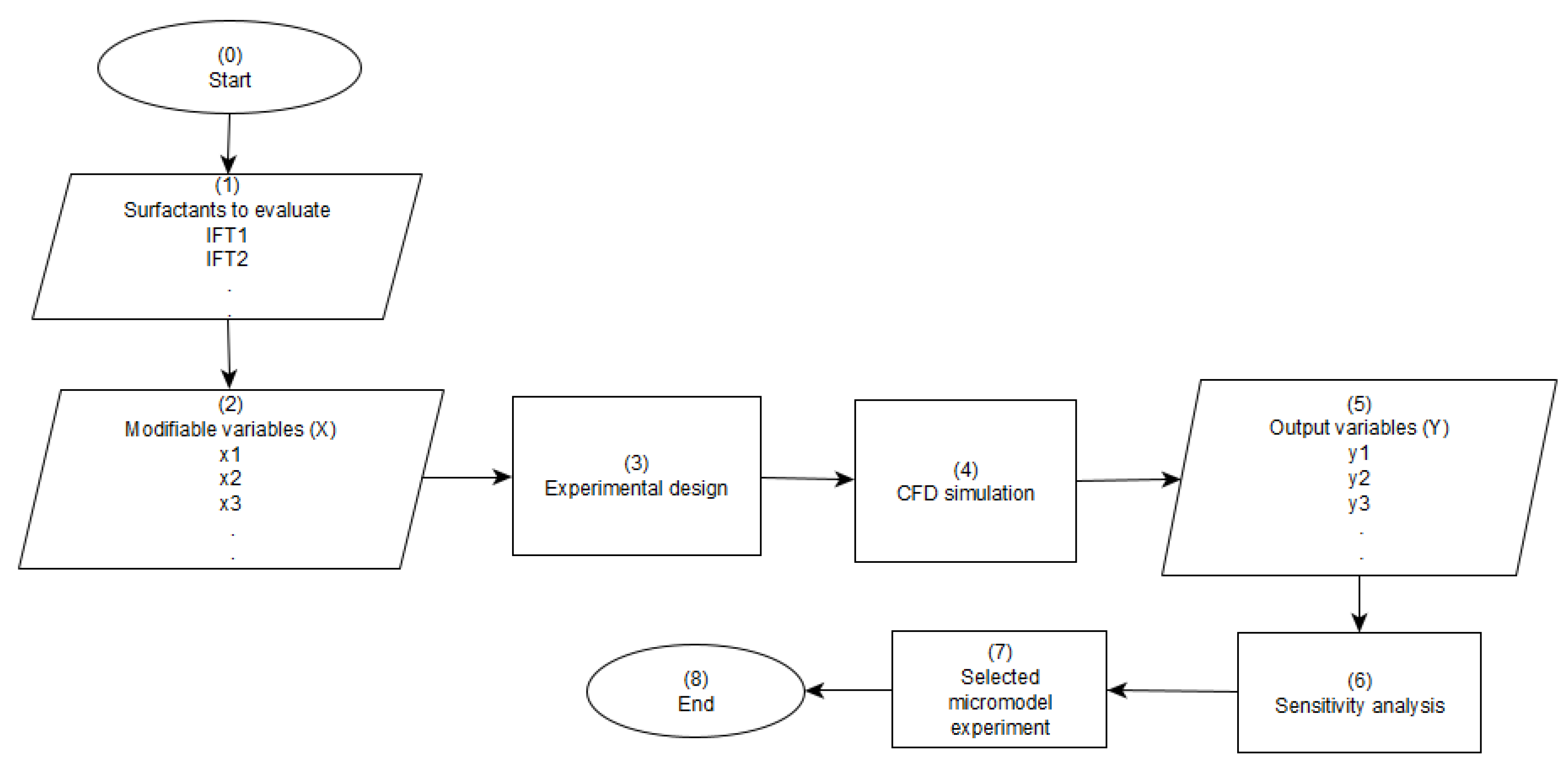
2. Towards a Micromodel Experiment Selection Flowchart
2.1. Surfactants
2.2. Modifiable Variables
2.3. Experimental Design
2.4. Sensitivity Analysis
3. Numerical Implementation
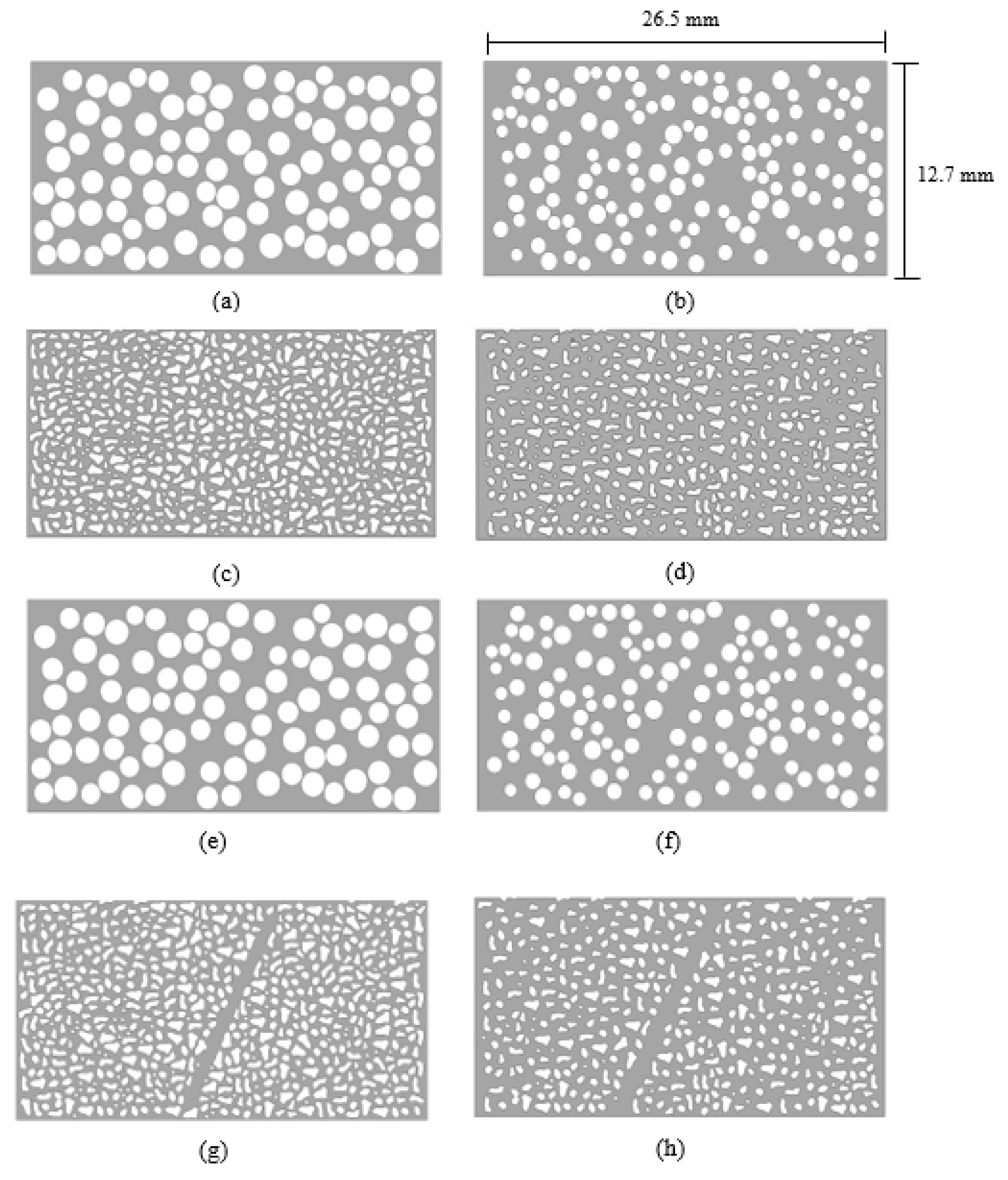
3.1. Geometry
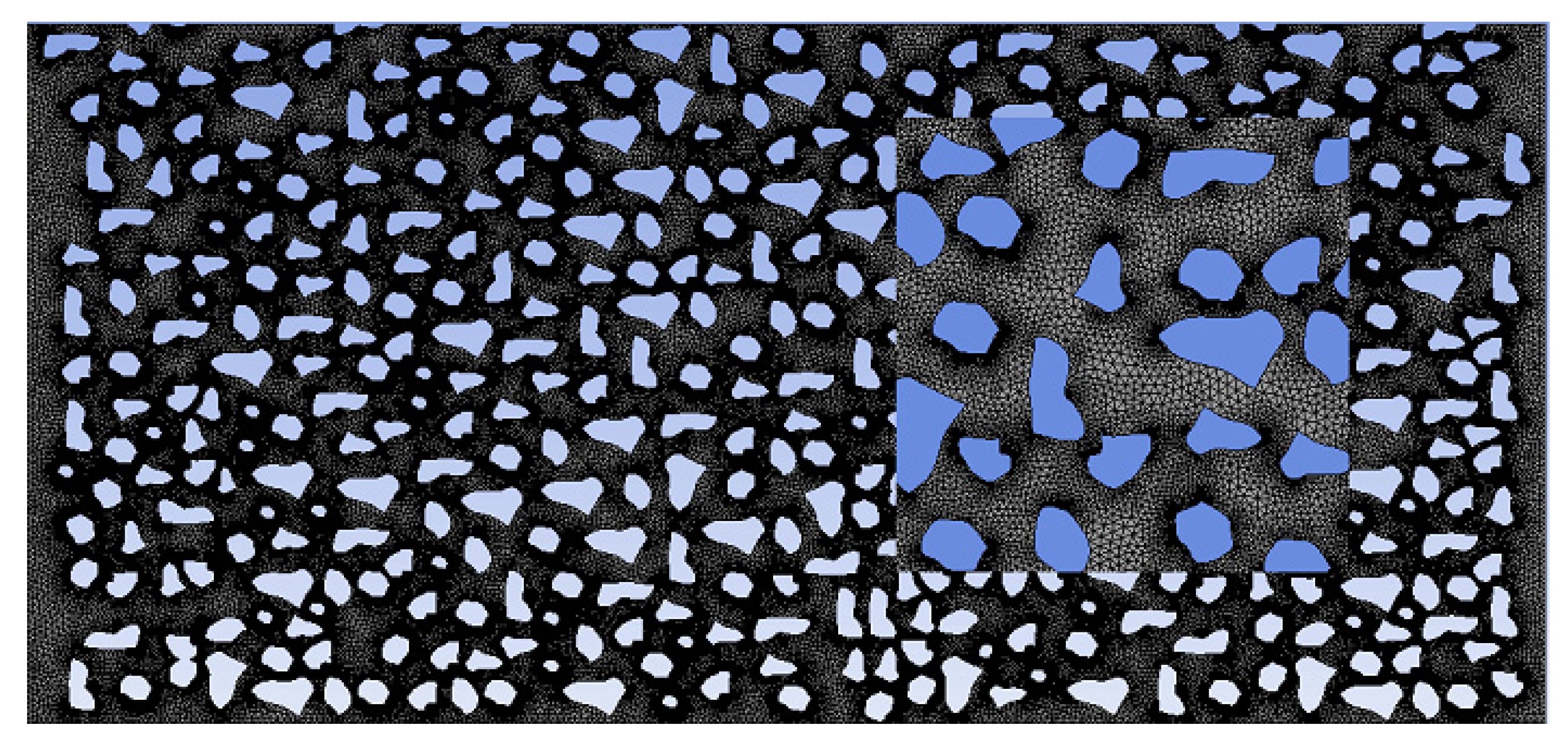
3.2. Mesh
3.3. CFD Implementation
- Intel® Xeon ® CPU E5-1620 v2 3.70 GHz
- 4 Cores
- 8 Logic processors
- 16.0 GB RAM
3.3.1. Governing Equations
3.3.2. Solver and Boundary Conditions
3.3.3. CFD Model Limitations
3.4. Evaluation of Output Variables
3.5. Fluid Properties
4. Results
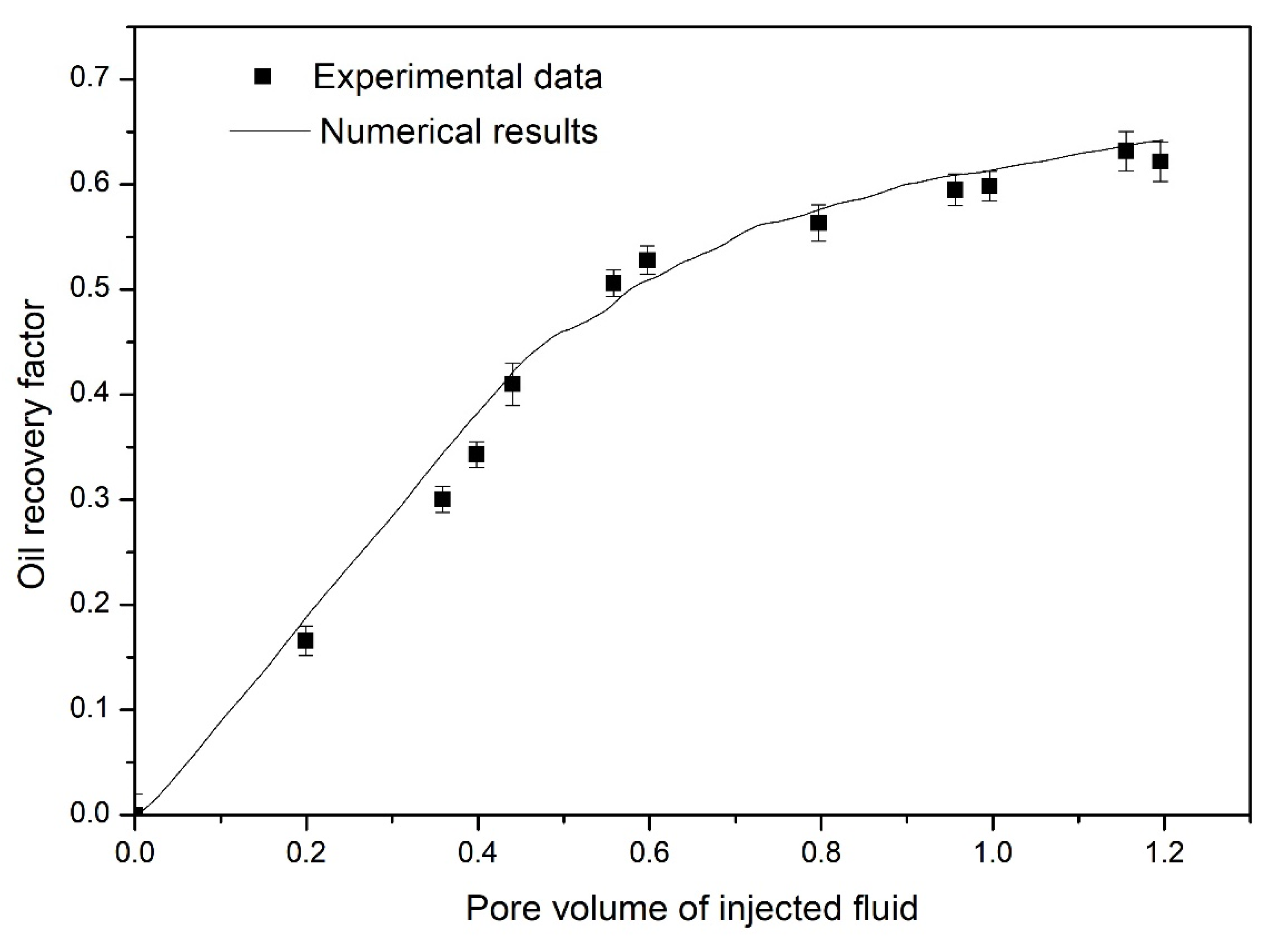
4.1. Validation of Numerical Results
4.2. Application of the Micromodel Experiment Selection Flowchart
5. Conclusions
Supplementary Materials
Author Contributions
Funding
Institutional Review Board Statement
Informed Consent Statement
Data Availability Statement
Acknowledgments
Conflicts of Interest
References
- Liu, Z.-x.; Liang, Y.; Wang, Q.; Guo, Y.-j.; Gao, M.; Wang, Z.-b.; Liu, W.-l. Status and progress of worldwide EOR field applications. J. Pet. Sci. Eng. 2020, 193, 107449. [Google Scholar] [CrossRef]
- Sheng, J.J. Status of surfactant EOR technology. Petroleum 2015, 1, 97–105. [Google Scholar] [CrossRef] [Green Version]
- Hanamertani, A.S.; Pilus, R.M.; Idris, A.K.; Irawan, S.; Tan, I.M. Ionic liquids as a potential additive for reducing surfactant adsorption onto crushed Berea sandstone. J. Pet. Sci. Eng. 2018, 162, 480–490. [Google Scholar] [CrossRef]
- Ahmadi, M.A.; Shadizadeh, S.R. Induced effect of adding nano silica on adsorption of a natural surfactant onto sandstone rock: Experimental and theoretical study. J. Pet. Sci. Eng. 2013, 112, 239–247. [Google Scholar] [CrossRef]
- Ahmadi, M.-A.; Ahmad, Z.; Phung, L.T.K.; Kashiwao, T.; Bahadori, A. Experimental investigation the effect of nanoparticles on micellization behavior of a surfactant: Application to EOR. Pet. Sci. Technol. 2016, 34, 1055–1061. [Google Scholar] [CrossRef]
- Amedi, H.; Ahmadi, M.-A. Experimental investigation the effect of nanoparticles on the oil-water relative permeability. Eur. Phys. J. Plus 2016, 131, 1–8. [Google Scholar] [CrossRef]
- Ahmadi, M.-A.; Shadizadeh, S.R. Nanofluid in hydrophilic state for EOR implication through carbonate reservoir. J. Dispers. Sci. Technol. 2014, 35, 1537–1542. [Google Scholar] [CrossRef]
- Ahmadi, M.A.; Sheng, J. Performance improvement of ionic surfactant flooding in carbonate rock samples by use of nanoparticles. Pet. Sci. 2016, 13, 725–736. [Google Scholar] [CrossRef] [Green Version]
- Ahmadi, M.A.; Shadizadeh, S.R. Nano-surfactant flooding in carbonate reservoirs: A mechanistic study. Eur. Phys. J. Plus 2017, 132, 1–13. [Google Scholar] [CrossRef]
- Ahmadi, M.A. Use of nanoparticles to improve the performance of sodium dodecyl sulfate flooding in a sandstone reservoir. Eur. Phys. J. Plus 2016, 131, 1–9. [Google Scholar] [CrossRef]
- Ahmadi, M.A.; Shadizadeh, S.R. Spotlight on the new natural surfactant flooding in carbonate rock samples in low salinity condition. Sci. Rep. 2018, 8, 1–15. [Google Scholar] [CrossRef] [Green Version]
- Ahmadi, M.A.; Shadizadeh, S.R. Adsorption of a nonionic surfactant onto a silica surface. Energy Sources Part A 2016, 38, 1455–1460. [Google Scholar] [CrossRef]
- Ahmadi, M.A.; Shadizadeh, S. Experimental and theoretical study of a new plant derived surfactant adsorption on quartz surface: Kinetic and isotherm methods. J. Dispers. Sci. Technol. 2015, 36, 441–452. [Google Scholar] [CrossRef]
- Ahmadi, M.A.; Galedarzadeh, M.; Shadizadeh, S.R. Wettability alteration in carbonate rocks by implementing new derived natural surfactant: Enhanced oil recovery applications. Transp. Porous Media 2015, 106, 645–667. [Google Scholar] [CrossRef]
- Keelan, D.; Koepf, E. The role of cores and core analysis in evaluation of formation damage. J. Pet. Technol. 1977, 29, 482–490. [Google Scholar] [CrossRef]
- Chapman, E.M. Microfluidic Visualisation and Analysis of Multiphase Flow Phenomena at the Pore Scale. Ph.D. Thesis, Imperial College London, London, UK, 2014. [Google Scholar]
- Cheraghian, G. An experimental study of surfactant polymer for enhanced heavy oil recovery using a glass micromodel by adding nanoclay. Pet. Sci. Technol. 2015, 33, 1410–1417. [Google Scholar] [CrossRef]
- Hematpour, H.; Arabjamloei, R.; Nematzadeh, M.; Esmaili, H.; Mardi, M. An experimental investigation of surfactant flooding efficiency in low viscosity oil using a glass micromodel. Energy Sources Part A 2012, 34, 1745–1758. [Google Scholar] [CrossRef]
- Hug, T.; Parrat, D.; Kunzi, P.-A.; Staufer, U.; Verpoorte, E.; de Rooij, N.F. Fabrication of nanochannels with PDMS, silicon and glass walls and spontaneous filling by capillary forces. In Proceedings of the 7th lnternational Conference on Miniaturized Chemical and Biochemical Analysts Systems, Squaw Valley, CA, USA, 5–9 October 2003. [Google Scholar]
- Kolari, K.; Saarela, V.; Franssila, S. Deep plasma etching of glass for fluidic devices with different mask materials. J. Micromech. Microeng. 2008, 18, 064010. [Google Scholar] [CrossRef]
- Rock, A.; Hincapie, R.; Wegner, J.; Ganzer, L. Advanced Flow Behavior Characterization of Enhanced Oil Recovery Polymers using Glass-Silicon-Glass Micromodels that Resemble Porous Media. In Proceedings of the SPE Europec Featured at 79th EAGE Conference and Exhibition, Paris, France, 12–15 June 2017. [Google Scholar]
- Wegner, M.; Christie, J. Chemical etching of deformation sub-structures in quartz. Phys. Chem. Miner. Vol. 1983, 9, 67–78. [Google Scholar] [CrossRef]
- Park, D.; Bou-Mikael, S.; King, S.; Thompson, K.; Willson, C.; Nikitopoulos, D. Design and fabrication of rock-based polymer micromodel. In Proceedings of the ASME 2012 International Mechanical Engineering Congress & Exposition, Houston, TX, USA, 9–15 November 2012; pp. 709–716. [Google Scholar]
- Mohammadi, F.; Haghtalab, A.; Jafari, A.; Gharibshahi, R. CFD study of surfactant flooding in a micromodel with quadratic pore shape. In Proceedings of the 1st National Conference on Oil and Gas Fields Development (OGFD), Tehran, Iran, 28–29 January 2015. [Google Scholar]
- Jafari, A.; Pour, S.E.F.; Gharibshahi, R. CFD Simulation of Biosurfactant Flooding into a Micromodel for Enhancing the Oil Recovery. Int. J. Chem. Eng. Appl. 2016, 7, 353–358. [Google Scholar] [CrossRef]
- Ghanad Dezfully, M.; Jafari, A.; Gharibshahi, R. CFD simulation of enhanced oil recovery using nanosilica/supercritical CO2. Adv. Mater. Res. 2015, 1104, 81–86. [Google Scholar] [CrossRef]
- Gharibshahi, R.; Jafari, A.; Ahmadi, H. CFD investigation of enhanced extra-heavy oil recovery using metallic nanoparticles/steam injection in a micromodel with random pore distribution. J. Pet. Sci. Eng. 2019, 174, 374–383. [Google Scholar] [CrossRef]
- Karadimitriou, N.; Hassanizadeh, S. A review of micromodels and their use in two-phase flow studies. Vadose Zone J. 2012, 11, vzj2011.0072. [Google Scholar] [CrossRef]
- Gharibshahi, R.; Jafari, A.; Haghtalab, A.; Karambeigi, M.S. Application of CFD to evaluate the pore morphology effect on nanofluid flooding for enhanced oil recovery. RSC Adv. 2015, 5, 28938–28949. [Google Scholar] [CrossRef]
- Clemens, T.; Tsikouris, K.; Buchgraber, M.; Castanier, L.M.; Kovscek, A. Pore-Scale Evaluation of Polymers Displacing Viscous Oil—Computational-Fluid-Dynamics Simulation of Micromodel Experiments. SPE Reserv. Eval. Eng. 2013, 16, 144–154. [Google Scholar] [CrossRef]
- Melchels, F.P.; Feijen, J.; Grijpma, D.W. A review on stereolithography and its applications in biomedical engineering. Biomaterials 2010, 31, 6121–6130. [Google Scholar] [CrossRef] [PubMed] [Green Version]
- Anbari, A.; Chien, H.T.; Datta, S.S.; Deng, W.; Weitz, D.A.; Fan, J. Microfluidic model porous media: Fabrication and applications. Small 2018, 14, 1703575. [Google Scholar] [CrossRef] [PubMed]
- Gerami, A.; Alzahid, Y.; Mostaghimi, P.; Kashaninejad, N.; Kazemifar, F.; Amirian, T.; Mosavat, N.; Warkiani, M.E.; Armstrong, R.T. Microfluidics for porous systems: Fabrication, microscopy and applications. Transp. Porous Media 2018, 130, 277–304. [Google Scholar] [CrossRef]
- Gerold, C.T.; Krummel, A.T.; Henry, C.S. Microfluidic devices containing thin rock sections for oil recovery studies. Microfluid. Nanofluid. 2018, 22, 76. [Google Scholar] [CrossRef]
- Gogoi, S.; Gogoi, S.B. Review on microfluidic studies for EOR application. J. Pet. Explor. Prod. Technol. 2019, 9, 2263–2277. [Google Scholar] [CrossRef] [Green Version]
- Lifton, V.A. Microfluidics: An enabling screening technology for enhanced oil recovery (EOR). Lab. Chip 2016, 16, 1777–1796. [Google Scholar] [CrossRef]
- Bergman, D.; Cire, A.A.; van Hoeve, W.-J.; Hooker, J. Decision Diagrams for Optimization; Springer: Berlin/Heidelberg, Germany, 2016; Volume 1. [Google Scholar]
- Shammay, A.; Evanson, I.E.J.; Stuetz, R.M. Selection framework for the treatment of sewer network emissions. J. Environ. Manag. 2019, 249, 109305. [Google Scholar] [CrossRef]
- Salman, B.; Salem, O.; He, S. Project-Level Sustainable Asphalt Roadway Treatment Selection Framework Featuring a Flowchart and Analytic Network Process. J. Transp. Eng. Part B 2020, 146, 04020041. [Google Scholar] [CrossRef]
- Gupta, A.; Kamat, D.; Shahrum, Z.; Firmansyah, A.; Salleh, N.; Tan, B.; Madon, B. Unique & practical approach in selection and classification of hydrocyclone desander technology: Utilizing a decade of experience. In Proceedings of the SPE/IATMI Asia Pacific Oil & Gas Conference and Exhibition, Jakarta, Indonesia, 17–19 October 2017. [Google Scholar]
- Trumm, D. Selection of passive AMD treatment systems-flow charts for New Zealand conditions. In Proceedings of the Australasian Institute of Mining and Metallurgy New Zealand Branch 40th Annual Conference, Christchurch, New Zealand, 13–15 August 2007. [Google Scholar]
- Priyanta, D.; Zaman, M. The development of a risk-based maintenance flowchart to select the correct methodology to develop maintenance strategies of oil and gas equipment. In Proceedings of the IOP Conference Series: Materials Science and Engineering, Suzhou, China, 17–19 March 2021; p. 012042. [Google Scholar]
- Bagheri, M.; Roshandel, R.; Shayegan, J. Optimal selection of an integrated produced water treatment system in the upstream of oil industry. Process Saf. Environ. Prot. 2018, 117, 67–81. [Google Scholar] [CrossRef]
- Gharibshahia, R.; Jafaria, A.; Haghtalaba, A.; Karambeigib, M.S. Simulation of nanofluid flooding in a micromodel with quadratic pore shape using CFD. In Proceedings of the 5th International Congress on Nanoscience & Nanotechnology, Tehran, Iran, 11 June 2014. [Google Scholar]
- Rostami, P.; Sharifi, M.; Aminshahidy, B.; Fahimpour, J. The effect of nanoparticles on wettability alteration for enhanced oil recovery: Micromodel experimental studies and CFD simulation. Pet. Sci. 2019, 16, 859–873. [Google Scholar] [CrossRef] [Green Version]
- Versteeg, H.K.; Malalasekera, W. An. Introduction to Computational Fluid Dynamics: The Finite Volume Method; Pearson Education: London, UK, 2007. [Google Scholar]
- Pires, J.C.; Alvim-Ferraz, M.C.; Martins, F.G. Photobioreactor design for microalgae production through computational fluid dynamics: A review. Renew. Sustain. Energy Rev. 2017, 79, 248–254. [Google Scholar] [CrossRef]
- Windt, C.; Davidson, J.; Ringwood, J.V. High-fidelity numerical modelling of ocean wave energy systems: A review of computational fluid dynamics-based numerical wave tanks. Renew. Sustain. Energy Rev. 2018, 93, 610–630. [Google Scholar] [CrossRef] [Green Version]
- Yu, H.; Engel, S.; Janiga, G.; Thévenin, D. A review of hemolysis prediction models for computational fluid dynamics. Artifial Organs 2017, 41, 603–621. [Google Scholar] [CrossRef] [Green Version]
- Park, H.W.; Yoon, W.B. Computational fluid dynamics (CFD) modelling and application for sterilization of foods: A review. Processes 2018, 6, 62. [Google Scholar] [CrossRef] [Green Version]
- Faizal, W.; Ghazali, N.; Khor, C.; Badruddin, I.A.; Zainon, M.; Yazid, A.A.; Ibrahim, N.B.; Razi, R.M. Computational fluid dynamics modelling of human upper airway: A review. Comput. Methods Programs Biomed. 2020, 196, 105627. [Google Scholar] [CrossRef] [PubMed]
- Toja-Silva, F.; Kono, T.; Peralta, C.; Lopez-Garcia, O.; Chen, J. A review of computational fluid dynamics (CFD) simulations of the wind flow around buildings for urban wind energy exploitation. J. Wind Eng. Ind. Aerodyn. 2018, 180, 66–87. [Google Scholar] [CrossRef]
- Tey, W.Y.; Asako, Y.; Sidik, N.A.C.; Goh, R.Z. Governing equations in computational fluid dynamics: Derivations and a recent review. Progress Energy Environ. 2017, 1, 1–19. [Google Scholar]
- Xu, G.; Luxbacher, K.D.; Ragab, S.; Xu, J.; Ding, X. Computational fluid dynamics applied to mining engineering: A review. Int. J. Min. Reclam. Environ. 2017, 31, 251–275. [Google Scholar] [CrossRef]
- Vavra, E.D.; Zeng, Y.; Xiao, S.; Hirasaki, G.J.; Biswal, S.L. Microfluidic Devices for Characterizing Pore-scale Event Processes in Porous Media for Oil Recovery Applications. J. Vis. Exp. 2018, 131, e56592. [Google Scholar] [CrossRef] [Green Version]
- Owete, O.S.; Brigham, W.E. Flow behavior of foam: A porous micromodel study. SPE Reserv. Eng. 1987, 2, 315–323. [Google Scholar] [CrossRef]
- Farzaneh, S.; Ghazanfari, M.; Kharrat, R.; Vossoughi, S. An experimental and numerical investigation of solvent injection to heavy oil in fractured five-spot micromodels. Pet. Sci. Technol. 2010, 28, 1567–1585. [Google Scholar] [CrossRef]
- Mohajeri, M.; Hemmati, M.; Shekarabi, A.S. An experimental study on using a nanosurfactant in an EOR process of heavy oil in a fractured micromodel. J. Pet. Sci. Eng. 2015, 126, 162–173. [Google Scholar] [CrossRef]
- Sedaghat, M.; Mohammadzadeh, O.; Kord, S.; Chatzis, I. Heavy oil recovery using ASP flooding: A pore-level experimental study in fractured five-spot micromodels. Can. J. Chem. Eng. 2016, 94, 779–791. [Google Scholar] [CrossRef]
- Wan, J.; Tokunaga, T.K.; Tsang, C.F.; Bodvarsson, G.S. Improved glass micromodel methods for studies of flow and transport in fractured porous media. Water Resour. Res. 1996, 32, 1955–1964. [Google Scholar] [CrossRef]
- Willingham, T.W.; Werth, C.J.; Valocchi, A.J. Evaluation of the effects of porous media structure on mixing-controlled reactions using pore-scale modeling and micromodel experiments. Environ. Sci. Technol. 2008, 42, 3185–3193. [Google Scholar] [CrossRef] [PubMed]
- Betancur, S.; Olmos, C.M.; Pérez, M.; Lerner, B.; Franco, C.A.; Riazi, M.; Gallego, J.; Carrasco-Marín, F.; Cortés, F.B. A microfluidic study to investigate the effect of magnetic iron core-carbon shell nanoparticles on displacement mechanisms of crude oil for chemical enhanced oil recovery. J. Pet. Sci. Eng. 2020, 184, 106589. [Google Scholar] [CrossRef]
- Lv, M.; Wang, S. Pore-scale modeling of a water/oil two-phase flow in hot water flooding for enhanced oil recovery. RSC Adv. 2015, 5, 85373–85382. [Google Scholar] [CrossRef]
- Zhao, J.; Wen, D. Pore-scale simulation of wettability and interfacial tension effects on flooding process for enhanced oil recovery. RSC Adv. 2017, 7, 41391–41398. [Google Scholar] [CrossRef] [Green Version]
- Goudarzi, B.; Mohammadmoradi, P.; Kantzas, A. Pore-level simulation of heavy oil reservoirs; competition of capillary, viscous, and gravity forces. In Proceedings of the SPE Latin America and Caribbean Heavy and Extra Heavy Oil Conference, Lima, Cyprus, 19–20 October 2016. [Google Scholar]
- Timgren, A.; Trägårdh, G.; Trägårdh, C. Effects of cross-flow velocity, capillary pressure and oil viscosity on oil-in-water drop formation from a capillary. Chem. Eng. Sci. 2009, 64, 1111–1118. [Google Scholar] [CrossRef]
- Zhao, J.; Yao, G.; Wen, D. Pore-scale simulation of water/oil displacement in a water-wet channel. Front. Chem. Sci. Eng. 2019, 13, 803–814. [Google Scholar] [CrossRef] [Green Version]
- Ferer, M.; Sams, W.N.; Geisbrecht, R.; Smith, D.H. Fractal nature of viscous fingering in two-dimensional pore level models. AIChE J. 1995, 41, 749–763. [Google Scholar] [CrossRef]
- Nittmann, J.; Daccord, G.; Stanley, H.E. Fractal growth viscous fingers: Quantitative characterization of a fluid instability phenomenon. Nature 1985, 314, 141–144. [Google Scholar] [CrossRef]
- Nabizadeh, A.; Adibifard, M.; Hassanzadeh, H.; Fahimpour, J.; Moraveji, M.K. Computational fluid dynamics to analyze the effects of initial wetting film and triple contact line on the efficiency of immiscible two-phase flow in a pore doublet model. J. Mol. Liq. 2019, 273, 248–258. [Google Scholar] [CrossRef]
- XU, K.; Zhu, P.; Tatiana, C.; Huh, C.; Balhoff, M. A microfluidic investigation of the synergistic effect of nanoparticles and surfactants in macro-emulsion based EOR. In Proceedings of the SPE Improved Oil Recovery Conference, Tulsa, OK, USA, 11–13 April 2016. [Google Scholar]
- Afsharpoor, A.; Balhoff, M.T.; Bonnecaze, R.; Huh, C. CFD modeling of the effect of polymer elasticity on residual oil saturation at the pore-scale. J. Pet. Sci. Eng. 2012, 94, 79–88. [Google Scholar] [CrossRef]
- Dong, M.; Liu, Q.; Li, A. Displacement mechanisms of enhanced heavy oil recovery by alkaline flooding in a micromodel. Particuology 2012, 10, 298–305. [Google Scholar] [CrossRef]
- Gutiérrez Pulido, H.; Vara Salazar, R.D.L. Análisis y Diseño de Experimentos; McGraw-Hill: New York, NY, USA, 2012. [Google Scholar]
- Ferrari, A.; Jimenez-Martinez, J.; Borgne, T.L.; Méheust, Y.; Lunati, I. Challenges in modeling unstable two-phase flow experiments in porous micromodels. Water Resour. Res. 2015, 51, 1381–1400. [Google Scholar] [CrossRef] [Green Version]
- Rosero, G.; Peñaherrera, A.; Olmos, C.; Boschan, A.; Granel, P.; Golmar, F.; Lasorsa, C.; Lerner, B.; Perez, M. Design and analysis of different models of microfluidic devices evaluated in Enhanced Oil Recovery (EOR) assays. Matéria 2018, 23, e12129. [Google Scholar] [CrossRef]
- Nilsson, M.A.; Kulkarni, R.; Gerberich, L.; Hammond, R.; Singh, R.; Baumhoff, E.; Rothstein, J.P. Effect of fluid rheology on enhanced oil recovery in a microfluidic sandstone device. J. Non-Newton. Fluid Mech. 2013, 202, 112–119. [Google Scholar] [CrossRef]
- Karambeigi, M.; Schaffie, M.; Fazaelipoor, M. Improvement of water flooding efficiency using mixed culture of microorganisms in heterogeneous micro-models. Pet. Sci. Technol. 2013, 31, 923–931. [Google Scholar] [CrossRef]
- Maaref, S.; Rokhforouz, M.R.; Ayatollahi, S. Numerical investigation of two phase flow in micromodel porous media: Effects of wettability, heterogeneity, and viscosity. Can. J. Chem. Eng. 2017, 95, 1213–1223. [Google Scholar] [CrossRef]
- Borji, M. Alkali-based Displacement Processes in Microfluidic Experiments: Application to the Matzen Oil Field. Ph.D. Thesis, Univeristy of Leoben, Leoben, Austria, 2017. [Google Scholar]
- Karadimitriou, N.K. Two-phase flow experimental studies in micro-models. Ph.D. Thesis, Faculty of Geosciences—UU Department of Earth Sciences, Utrecht, The Netherlands, 2013. [Google Scholar]
- Cui, J.; Babadagli, T. Use of new generation chemicals and nano materials in heavy-oil recovery: Visual analysis through micro fluidics experiments. Colloids Surf. A 2017, 529, 346–355. [Google Scholar] [CrossRef]
- Yarveicy, H.; Javaheri, A. Application of Lauryl Betaine in enhanced oil recovery: A comparative study in micromodel. Petroleum 2019, 5, 123–127. [Google Scholar] [CrossRef]
- ANSYS. ANSYS Fluent Theory Guide; ANSYS: Canonsburg, PA, USA, 2013. [Google Scholar]
- Brackbill, J.U.; Kothe, D.B.; Zemach, C. A continuum method for modeling surface tension. J. Comput. Phys. 1992, 100, 335–354. [Google Scholar] [CrossRef]
- Levitt, D.; Jackson, A.; Heinson, C.; Britton, L.N.; Malik, T.; Dwarakanath, V.; Pope, G.A. Identification and evaluation of high-performance EOR surfactants. In Proceedings of the SPE/DOE Symposium on Improved Oil Recovery, Tulsa, OK, USA, 22–26 April 2006. [Google Scholar]
- Belhaj, A.F.; Elraies, K.A.; Mahmood, S.M.; Zulkifli, N.N.; Akbari, S.; Hussien, O.S. The effect of surfactant concentration, salinity, temperature, and pH on surfactant adsorption for chemical enhanced oil recovery: A review. J. Pet. Explor. Prod. Technol. 2020, 10, 125–137. [Google Scholar] [CrossRef] [Green Version]
- Haghshenasfard, M.; Hooman, K. CFD modeling of asphaltene deposition rate from crude oil. J. Pet. Sci. Eng. 2015, 128, 24–32. [Google Scholar] [CrossRef]
- Roudsari, S.F.; Turcotte, G.; Dhib, R.; Ein-Mozaffari, F. CFD modeling of the mixing of water in oil emulsions. Comput. Chem. Eng. 2012, 45, 124–136. [Google Scholar] [CrossRef]
- Falconer, K. Fractal Geometry: Mathematical Foundations and Applications; John Wiley & Sons: Hoboken, NJ, USA, 2004. [Google Scholar]
- Olmos, C.M.; Vaca, A.; Rosero, G.; Peñaherrera, A.; Perez, C.; de Sá Carneiro, I.; Vizuete, K.; Arroyo, C.R.; Debut, A.; Pérez, M.S. Epoxy resin mold and PDMS microfluidic devices through photopolymer flexographic printing plate. Sens. Actuators B 2019, 288, 742–748. [Google Scholar] [CrossRef]
- Neuman, S.P. Theoretical derivation of Darcy’s law. Acta Mech. 1977, 25, 153–170. [Google Scholar] [CrossRef]
- Moore, T.; Slobod, R. Displacement of oil by water-effect of wettability, rate, and viscosity on recovery. In Proceedings of the Fall Meeting of the Petroleum Branch of AIME, New Orleans, LA, USA, 2–5 October 1955. [Google Scholar]


| Porosity | Grain Shape | Presence of Preferential Flowing Channel | Preferential Flowing Channel Configuration | Heterogeneity | Tortuosity | Injection Velocity | Pore Shape | Pore-throat Connectivity | ||
|---|---|---|---|---|---|---|---|---|---|---|
| Oil recovery factor | ||||||||||
| Pressure drop | ||||||||||
| Fractal dimension | ||||||||||
| Breakthrough time | ||||||||||
| Viscosity | ||||||||||
| Displacement micro-mechanisms | ||||||||||
| Emulsion formation | ||||||||||
| Drops shape | ||||||||||
| Fluid distribution | ||||||||||
| Grain Shape | Porosity | Injection Velocity (ft/day) | Presence of Preferential Flowing Channel | IFT (mN/m) | Capillary Number | Breakthrough Time (PVI) | Recovery Factor | Fractal Dimension | Pressure Drop (Pa) | Entrapment Effect |
|---|---|---|---|---|---|---|---|---|---|---|
| circular | 0.5 | 10 | no | 0.037 | 0.013 | 0.4351 | 0.3882 | 1.5666 | 9.0840 | 0.0326 |
| irregular | 0.5 | 10 | no | 0.037 | 0.013 | 0.4069 | 0.3944 | 1.6281 | 42.1359 | 0.0429 |
| circular | 0.7 | 10 | no | 0.037 | 0.013 | 0.4112 | 0.3979 | 1.6610 | 3.5700 | 0.0411 |
| irregular | 0.7 | 10 | no | 0.037 | 0.013 | 0.4407 | 0.4100 | 1.7155 | 7.1765 | 0.0844 |
| circular | 0.5 | 30 | no | 0.037 | 0.039 | 0.4274 | 0.3800 | 1.5743 | 25.2136 | 0.0367 |
| irregular | 0.5 | 30 | no | 0.037 | 0.039 | 0.3829 | 0.3797 | 1.6428 | 117.325 | 0.0439 |
| circular | 0.7 | 30 | no | 0.037 | 0.039 | 0.3954 | 0.3832 | 1.6394 | 9.5758 | 0.0345 |
| irregular | 0.7 | 30 | no | 0.037 | 0.039 | 0.4476 | 0.4135 | 1.7102 | 19.2405 | 0.0974 |
| circular | 0.5 | 10 | yes | 0.037 | 0.013 | 0.4227 | 0.3855 | 1.5880 | 9.4705 | 0.0579 |
| irregular | 0.5 | 10 | yes | 0.037 | 0.013 | 0.3992 | 0.3785 | 1.6251 | 41.8144 | 0.0517 |
| circular | 0.7 | 10 | yes | 0.037 | 0.013 | 0.4127 | 0.4027 | 1.6871 | 3.1050 | 0.0394 |
| irregular | 0.7 | 10 | yes | 0.037 | 0.013 | 0.4426 | 0.4069 | 1.6933 | 6.7786 | 0.0788 |
| circular | 0.5 | 30 | yes | 0.037 | 0.039 | 0.4031 | 0.3662 | 1.5834 | 26.1504 | 0.0151 |
| irregular | 0.5 | 30 | yes | 0.037 | 0.039 | 0.3563 | 0.3390 | 1.6192 | 127.808 | 0.0708 |
| circular | 0.7 | 30 | yes | 0.037 | 0.039 | 0.4245 | 0.4135 | 1.6763 | 8.6735 | 0.0554 |
| irregular | 0.7 | 30 | yes | 0.037 | 0.039 | 0.4484 | 0.4093 | 1.7125 | 19.1542 | 0.1001 |
| circular | 0.5 | 10 | no | 0.045 | 0.011 | 0.4322 | 0.3861 | 1.5767 | 8.9602 | 0.0368 |
| irregular | 0.5 | 10 | no | 0.045 | 0.011 | 0.4392 | 0.4054 | 1.6229 | 42.6613 | 0.0491 |
| circular | 0.7 | 10 | no | 0.045 | 0.011 | 0.4045 | 0.3927 | 1.6627 | 3.5694 | 0.0408 |
| irregular | 0.7 | 10 | no | 0.045 | 0.011 | 0.4470 | 0.4178 | 1.7228 | 7.2455 | 0.0652 |
| circular | 0.5 | 30 | no | 0.045 | 0.032 | 0.4393 | 0.3906 | 1.5623 | 24.8362 | 0.0355 |
| irregular | 0.5 | 30 | no | 0.045 | 0.032 | 0.3705 | 0.3608 | 1.6484 | 119.187 | 0.0725 |
| circular | 0.7 | 30 | no | 0.045 | 0.032 | 0.4501 | 0.4325 | 1.6664 | 9.5706 | 0.0433 |
| irregular | 0.7 | 30 | no | 0.045 | 0.032 | 0.4257 | 0.3946 | 1.7056 | 20.9500 | 0.0935 |
| circular | 0.5 | 10 | yes | 0.045 | 0.011 | 0.4306 | 0.3938 | 1.5859 | 9.3153 | 0.0640 |
| irregular | 0.5 | 10 | yes | 0.045 | 0.011 | 0.3882 | 0.3702 | 1.6110 | 43.8324 | 0.0621 |
| circular | 0.7 | 10 | yes | 0.045 | 0.011 | 0.4183 | 0.4079 | 1.6742 | 3.1890 | 0.0398 |
| irregular | 0.7 | 10 | yes | 0.045 | 0.011 | 0.4468 | 0.4106 | 1.7297 | 7.0466 | 0.0766 |
| circular | 0.5 | 30 | yes | 0.045 | 0.032 | 0.4075 | 0.3758 | 1.5831 | 26.0617 | 0.0757 |
| irregular | 0.5 | 30 | yes | 0.045 | 0.032 | 0.3623 | 0.3457 | 1.6378 | 124.657 | 0.0558 |
| circular | 0.7 | 30 | yes | 0.045 | 0.032 | 0.4303 | 0.4182 | 1.6680 | 8.7053 | 0.0528 |
| irregular | 0.7 | 30 | yes | 0.045 | 0.032 | 0.4386 | 0.4031 | 1.7209 | 20.4482 | 0.0944 |
| Micromodel | Grain Shape | Porosity | Presence of Preferential Flowing Channel |
|---|---|---|---|
| a | Circular | 0.5 | no |
| b | Circular | 0.7 | no |
| c | Irregular | 0.5 | no |
| d | Irregular | 0.7 | no |
| e | Circular | 0.5 | yes |
| f | Circular | 0.7 | yes |
| g | Irregular | 0.5 | yes |
| h | Irregular | 0.7 | yes |
| Micromodel | Number of Grid | Number of Cells | Number of Nodes | ni/n0 | ΔP (Pa.) | |
|---|---|---|---|---|---|---|
| a | 1 | 106232 | 82422 | 1.0 | 0.0175 | |
| 2 | 178656 * | 118890 | 1.7 | 0.0166 | 0.051 | |
| 3 | 683801 | 372377 | 6.4 | 0.0161 | 0.034 | |
| b | 1 | 83248 | 51722 | 1.0 | 0.0068 | |
| 2 | 146637 * | 83689 | 1.7 | 0.0064 | 0.059 | |
| 3 | 379198 | 200661 | 4.5 | 0.0063 | 0.022 | |
| c | 1 | 253863 | 143892 | 1.0 | 0.0954 | |
| 2 | 411068 * | 227317 | 1.7 | 0.0777 | 0.229 | |
| 3 | 1163110 | 617919 | 4.5 | 0.0761 | 0.020 | |
| d | 1 | 134200 | 74919 | 1.0 | 0.0137 | |
| 2 | 324776 * | 175961 | 2.4 | 0.0128 | 0.073 | |
| 3 | 701344 | 36823 | 5.2 | 0.0127 | 0.005 | |
| e | 1 | 94784 | 76642 | 1.0 | 0.0218 | |
| 2 | 155622 * | 107304 | 1.6 | 0.0186 | 0.171 | |
| 3 | 335658 | 197753 | 3.5 | 0.0179 | 0.042 | |
| f | 1 | 106986 | 63755 | 1.0 | 0.0083 | |
| 2 | 218876 * | 120112 | 2.1 | 0.0074 | 0.122 | |
| 3 | 378635 | 200444 | 3.6 | 0.0070 | 0.058 | |
| g | 1 | 252252 | 143061 | 1.0 | 0.0941 | |
| 2 | 408536 * | 226044 | 1.7 | 0.0807 | 0.166 | |
| 3 | 1169517 | 620897 | 4.7 | 0.0777 | 0.039 | |
| h | 1 | 133312 | 74410 | 1.0 | 0.0150 | |
| 2 | 320726 * | 173874 | 2.4 | 0.0134 | 0.125 | |
| 3 | 694060 | 364896 | 5.2 | 0.0129 | 0.039 |
| Fluid | Density (kg/m3) | k | n | Maximum Viscosity (Pa∙s) | Minimum Viscosity (Pa∙s) |
|---|---|---|---|---|---|
| Surfactant solution | 1084.3 | 0.028 | 0.638 | 0.017 | 0.005 |
| Oil | 926.5 | 0.103 | 0.977 | 0.099 | 0.092 |
| Case | Grain Shape | Presence of Preferential Flowing Channel | Porosity | Injection Velocity (ft/day) | ||||||
|---|---|---|---|---|---|---|---|---|---|---|
| 1 | circular | no | 0.5 | 10 | 0.59 | 0.80 | 0.73 | 0.12 | 5.17 | 7.41 |
| circular | no | 0.7 | 10 | 1.49 | 1.85 | 0.12 | 0.00 | 0.42 | 3.88 | |
| circular | no | 0.5 | 30 | 3.05 | 3.31 | 0.87 | 0.37 | 1.51 | 9.12 | |
| circular | no | 0.7 | 30 | 14.24 | 15.18 | 1.95 | 0.01 | 11.01 | 42.38 | |
| 2 | irregular | no | 0.5 | 10 | 3.18 | 8.97 | 0.38 | 0.51 | 7.72 | 20.75 |
| irregular | no | 0.7 | 10 | 2.23 | 1.74 | 0.53 | 0.07 | 23.94 | 28.51 | |
| irregular | no | 0.5 | 30 | 5.40 | 3.43 | 0.41 | 1.82 | 35.76 | 46.85 | |
| irregular | no | 0.7 | 30 | 5.48 | 6.10 | 0.33 | 1.67 | 4.83 | 18.42 | |
| 3 | circular | yes | 0.5 | 10 | 2.40 | 2.19 | 0.15 | 0.15 | 7.67 | 12.56 |
| circular | yes | 0.7 | 10 | 1.50 | 1.57 | 0.93 | 0.08 | 0.44 | 4.53 | |
| circular | yes | 0.5 | 30 | 2.76 | 1.22 | 0.02 | 0.09 | 75.58 | 79.68 | |
| circular | yes | 0.7 | 30 | 1.36 | 1.62 | 0.60 | 0.03 | 3.23 | 6.84 | |
| 4 | irregular | yes | 0.5 | 10 | 2.41 | 3.06 | 1.02 | 1.97 | 13.04 | 21.50 |
| irregular | yes | 0.7 | 10 | 1.07 | 1.16 | 2.63 | 0.26 | 2.75 | 7.87 | |
| irregular | yes | 0.5 | 30 | 1.93 | 1.67 | 1.34 | 3.08 | 18.72 | 26.74 | |
| irregular | yes | 0.7 | 30 | 1.79 | 2.72 | 0.61 | 1.27 | 7.12 | 13.50 |
| Case | Recovery Factor | Breakthrough Time | Fractal Dimension | Pressure Drop Change | Entrapment Effect | |||||
|---|---|---|---|---|---|---|---|---|---|---|
| Major Change | Minor Change | Major Change | Minor Change | Major Change | Minor Change | Major Change | Minor Change | Major Change | Minor Change | |
| 1: Circular grain shape and non-preferential channel micromodel | High injection velocity—High porosity | Low injection velocity—Low porosity | High injection velocity—High porosity | Low injection velocity—Low porosity | High injection velocity—High porosity | Low injection velocity—High porosity | High injection velocity—Low porosity | High injection velocity—High porosity | High injection velocity—High porosity | Low injection velocity—High porosity |
| 2: Irregular grain shape and non-preferential channel micromodel | High injection velocity | Low injection velocity | Low injection velocity—Low porosity | Low injection velocity—High porosity | Low injection velocity—High porosity | High injection velocity—High porosity | High injection velocity—Low porosity | Low injection velocity—High porosity | High injection velocity—Low porosity | High injection velocity -High porosity |
| 3: Circular grain shape and preferential channel micromodel | Low injection velocity—Low porosity | High injection velocity—High porosity | Low injection velocity—Low porosity | High injection velocity—Low porosity | Low injection velocity—High porosity | High injection velocity—Low porosity | Low injection velocity—Low porosity | High injection velocity—High porosity | High injection velocity—Low porosity | Low injection velocity—High porosity |
| 4: Irregular grain shape and preferential channel micromodel | Low injection velocity—Low porosity | Low injection velocity—High porosity | Low injection velocity—Low porosity | Low injection velocity—High porosity | Low injection velocity—High porosity | High injection velocity—High porosity | High injection velocity—Low porosity | Low injection velocity—High porosity | High injection velocity—Low porosity | Low injection velocity—High porosity |
| Case | Changes Considering the Effect of all Response Variables (Y) | |
|---|---|---|
| Major Change | Minor Change | |
| 1: Circular grain shape and non-preferential flowing channel micromodel | High injection velocity—High porosity | Low injection velocity—High porosity |
| 2: Irregular grain shape and non-preferential flowing channel micromodel | High injection velocity—Low porosity | High injection velocity—High porosity |
| 3: Circular grain shape and preferential flowing channel micromodel | High injection velocity–Low porosity | Low injection velocity – High porosity |
| 4: Irregular grain shape and preferential flowing channel micromodel | High injection velocity—Low porosity | Low injection velocity—High porosity |
Publisher’s Note: MDPI stays neutral with regard to jurisdictional claims in published maps and institutional affiliations. |
© 2021 by the authors. Licensee MDPI, Basel, Switzerland. This article is an open access article distributed under the terms and conditions of the Creative Commons Attribution (CC BY) license (https://creativecommons.org/licenses/by/4.0/).
Share and Cite
Céspedes, S.; Molina, A.; Lerner, B.; Pérez, M.S.; Franco, C.A.; Cortés, F.B. A Selection Flowchart for Micromodel Experiments Based on Computational Fluid Dynamic Simulations of Surfactant Flooding in Enhanced Oil Recovery. Processes 2021, 9, 1887. https://doi.org/10.3390/pr9111887
Céspedes S, Molina A, Lerner B, Pérez MS, Franco CA, Cortés FB. A Selection Flowchart for Micromodel Experiments Based on Computational Fluid Dynamic Simulations of Surfactant Flooding in Enhanced Oil Recovery. Processes. 2021; 9(11):1887. https://doi.org/10.3390/pr9111887
Chicago/Turabian StyleCéspedes, Santiago, Alejandro Molina, Betiana Lerner, Maximiliano S. Pérez, Camilo A. Franco, and Farid B. Cortés. 2021. "A Selection Flowchart for Micromodel Experiments Based on Computational Fluid Dynamic Simulations of Surfactant Flooding in Enhanced Oil Recovery" Processes 9, no. 11: 1887. https://doi.org/10.3390/pr9111887