1. Introduction
The amount of energy consumed by various pumps accounts for more than 12% of the total energy consumption every year. The mixed-flow pumps are increasingly being used in industrial processes and agriculture due to their efficient hydraulic performance. Therefore, it is necessary to provide a reliable and effective optimization design method for further improving the performance of the mixed-flow pump.
The current and commonly used impeller combination optimization system is composed of the following five parts: Impeller geometric parameters, computational fluid dynamics (CFD) analyses, design of experiment (DOE), approximate model and optimization algorithm. The geometric parameters are used to describe the spatial shape of the impeller; CFD is used to calculate the performance of the impeller; DOE is used to create the database samples; the approximate model is used to construct the function relationship between the design variables and optimization objectives, and the optimization algorithm is used to solve the approximate model to obtain an optimal solution set in the entire design space. The effectiveness of this optimization system has been verified in a large number of optimization designs. Suh et al. [
1] improved the efficiency and cavitation performance of a mixed-flow pump at the design point by combining the use of the central composite design (CCD), RSM, and sequence quadratic program (SQP) to change the impeller geometric parameters. Kim et al. [
2], also solved the head overdesigned problem and improved the efficiency of a mixed-flow pump at design point by combined application of CCD and RSM to modify the impeller and diffuser inlet angle. Furthermore, Pei et al. [
3] enlarged the high efficiency area of a centrifugal pump by combined using the LHS method, RSM, and NSGA-Ⅱ to change the meridional shape. The stability, efficiency, and cavitation performance of a centrifugal pump were improved by combined applications of LHS, kriging model, and NSGA-Ⅱ to modify the meridional shape [
4,
5]. Miao et al. [
6] increased the efficiency and cavitation performance of axial-flow pump by combined usage of Group method of date handing type neural networks and modified PSO to improve the meridional shape. Meng et al. [
7] optimized the reversible axial-flow pump by increasing the reverse pump performance with a slight decrease in the forward pump performance by combining LHS, artificial neural network (ANN) and NSGA-Ⅱ to improve the main geometric parameters of impeller and diffuser.
However, this optimization system is associated with challenges such as, to accurately describe the 3D shape of the impeller, a large number of geometric parameters are required. Moreover, there exists no direct relationship between the geometric parameters and the hydraulic performance of the impeller [
8]. Although the sensitivity tests can be used to reduce the number of design parameters, the upper limit of the optimization design drops accordingly. Therefore, a more suitable method of impeller parameterization is needed.
A feasible solution to this problem is to use the IDM to parameterize the impeller [
9,
10,
11]. The three main design parameters in IDM are the blade loading along the meridional shape at the hub and shroud, the stacking at the trailing edge of the blade, and the circulation along the spanwise at the exit of the impeller. Compared with the traditional parameterization method based on geometry parameters, the IDM has the advantages of fewer design parameters and the design parameters are more closely related to the hydrodynamic performance [
12,
13]. In addition, the blade angle in IDM is directly computed by the given design parameters, which is quite different from the results obtained by the conformal transformation in the traditional design [
14]. The effectiveness of IDM has been widely proven in the optimization design of various turbomachinery. Zhu et al. [
15,
16,
17] improved the efficiency, cavitation and stability performance of a pump-turbine runner by varying the blade loading and stacking by combined using the LHS, RSM, and NSGA-Ⅱ. Bonaiuti et al. [
18] increased the high efficiency area of a compressor by changing the blade loading, stacking and spanwise circulation by combined using DOE and RSM. Lee et al. [
19] improved the efficiency and pressure rise of an axial fan by considering the blade loading, stacking and spanwise circulation by the combined application DOE and RSM.
There is a common point in the previous studies which is, a constant value of circulation from hub to shroud (free vortex) is imposed at impeller exit, and only a few studies used a linear spanwise distribution (forced vortex) at the impeller exit. However, Lang et al. [
20] and Chen [
21] through the theoretical derivations show that the best spanwise distribution of impeller exit circulation (SDIEC) is a non-linear distribution. Zhang et al. [
22,
23] proved the correctness of the theoretical derivation through the experimental measurement of a series of high-efficiency pumps. The author’s previous work also showed that in the multi-points and multi-objective optimization of mixed-flow pump impeller, there are some better non-linear SDIEC than the linear distribution.
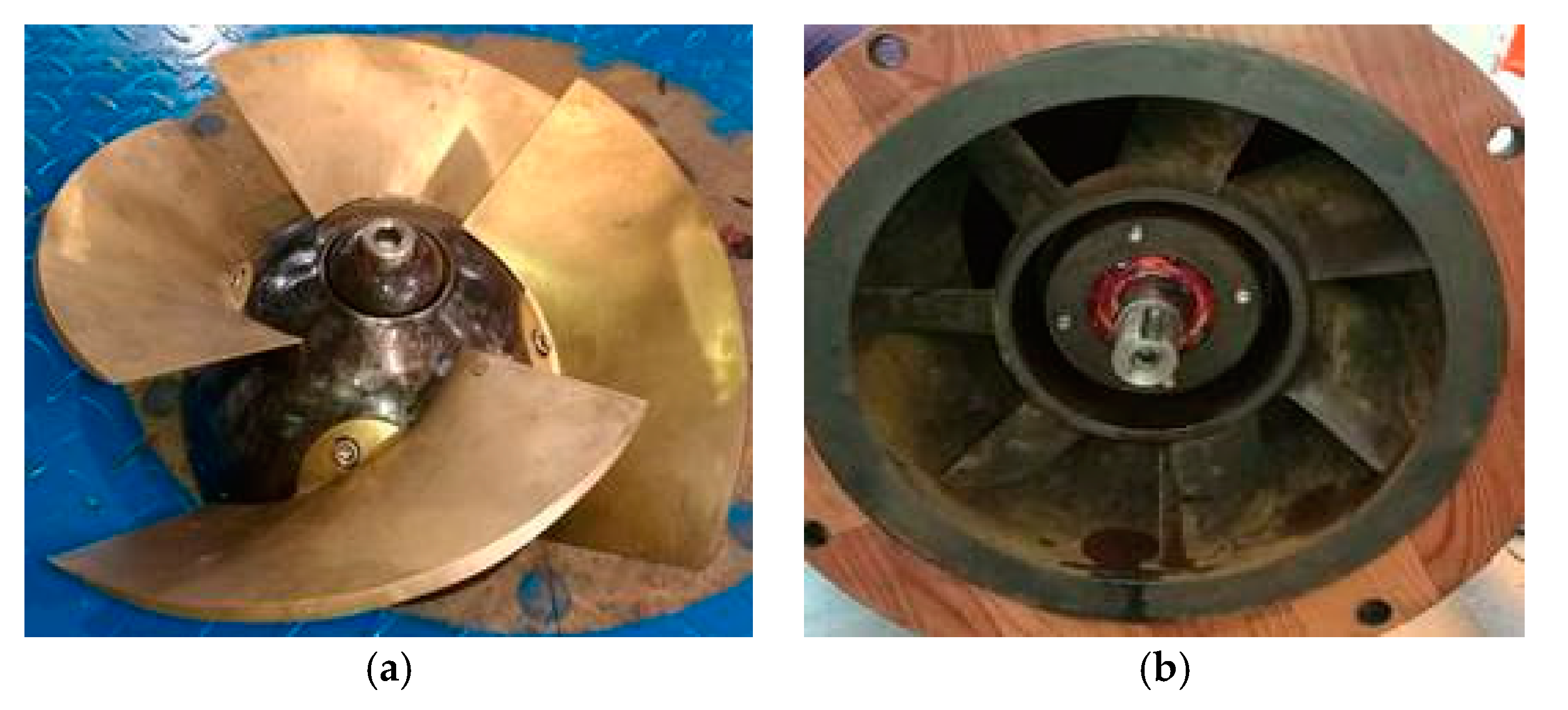
In this study, a widely used mixed-flow pump impeller is comprehensively improved by using the combination optimization system based on IDM after considering the effect of SDIEC on the impeller performance. Firstly, the mixed-flow pump design specifications and the optimization design system are introduced. Secondly, the optimization system was applied to design a series of impeller and a preferred impeller was selected. Finally, the flow field characteristics in the preferred impeller and the original impeller are compared, and the main effect of each parameter to the optimization objective was analyzed.
3. Optimization Design System
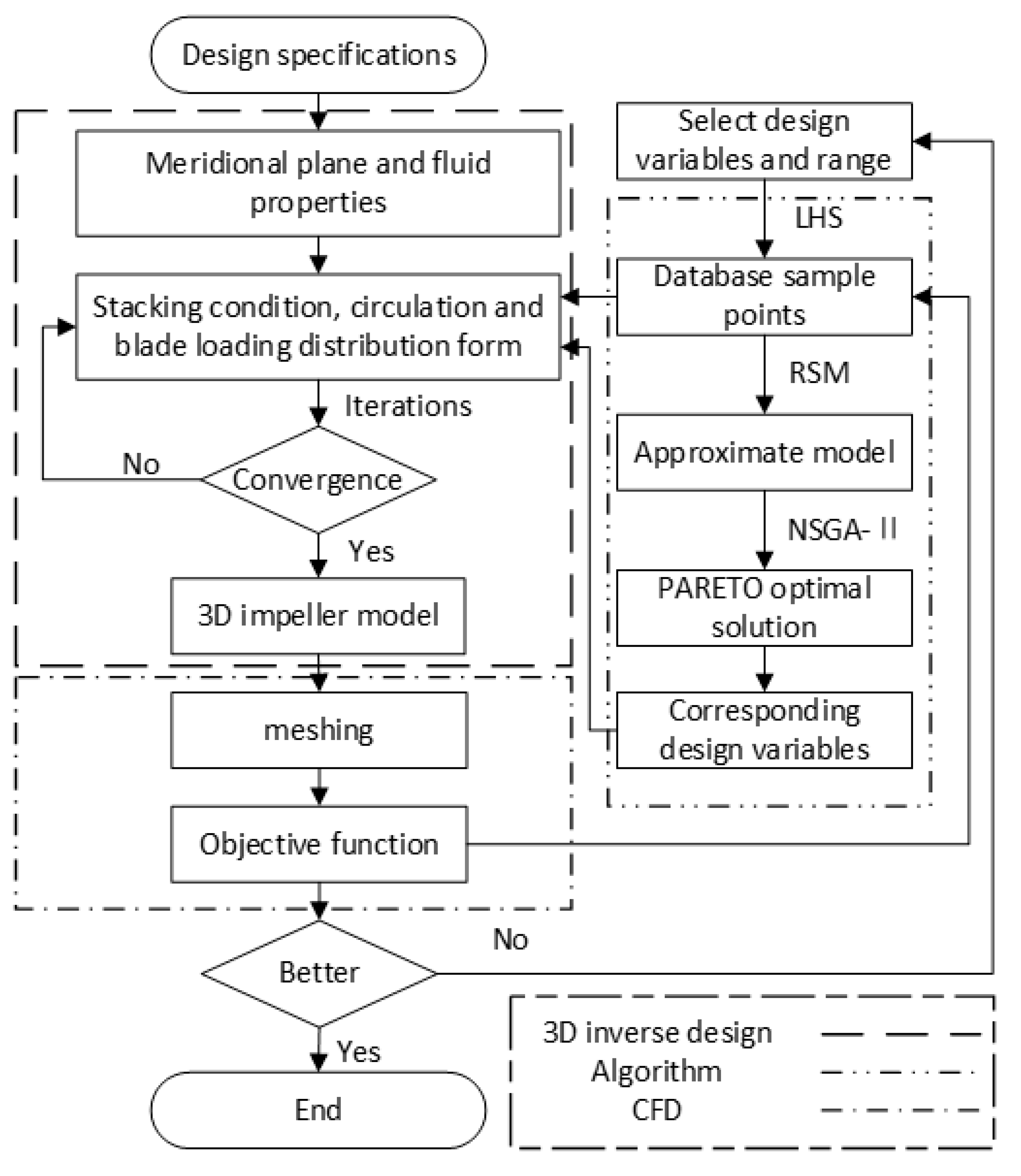
The combination optimization system was constructed by the CFD analyses, IDM, LHS, RSM, and NSGA-Ⅱ. The flow chart of this optimization system is shown in
Figure 2.
3.1. CFD Analyses
In this system, CFD analyses were employed to calculate the optimization objectives and validate the results of optimization. Thus, how to ensure the accuracy of CFD analyses become a key point for the optimization process. The widely used commercial software ANSYS (2019 R3, AnShiYaTai, Beijing, China) which is a large-scale general finite element analyses (FEA) software was utilized for performance estimation and inner flow-field analyses.
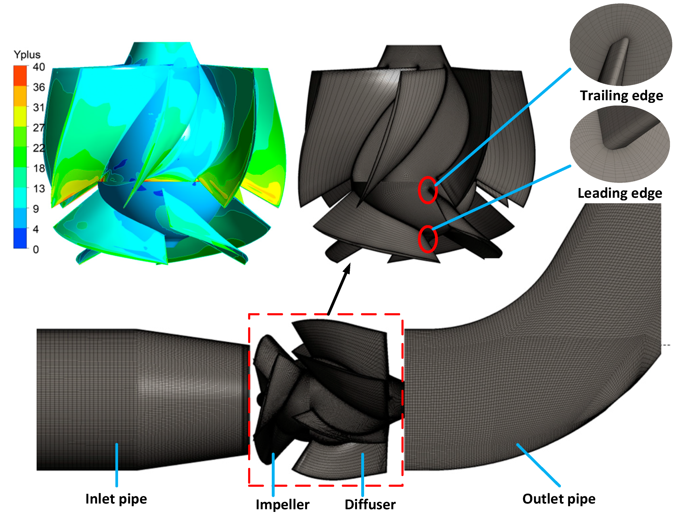
Structured grids were used in all calculation domains as shown in
Figure 3. The structured grids of the impeller and vane diffuser were generated by ANSYS TurboGrid while that of the inlet and outlet pipes were generated by ANSYS ICEM. The pump efficiency and head at design point were selected for the grid independence analysis (See
Table 2). Considering the effect of the number of grids on the accuracy of calculation results and the computational resources available, Mesh 3 is adopted for the CFD simulations. Meanwhile, the maximum Y+ of impeller and diffuser blade surface does not exceed 40 as shown in
Figure 3.
The 3D Reynolds-Averaged Navier–Stokes (RANS) equations and energy equations were used to analyze the incompressible flows in the pump. The governing equations were discretized by the finite volume method. The
shear stress transport (SST) model was selected as a closure of the RANS equation since it can accurately predict the flow separation in the pump [
24]. The convection–diffusion equation was solved by a high-resolution scheme. “Mass Flow Rate” was set at the inlet boundary while ‘Static Pressure’ was set at outlet boundary. “Frozen rotor” was set at interfaces between the inlet pipe to impeller and impeller to vane diffuser. The no-slip condition was applied to all walls and the Root mean square residual values of mass and all directions of the momentum were set as
.
3.2. 3D Inverse Design Method
In IDM (Turbodesign 6.4.0, ADT, Shanghai, China, 2020), the inlet flow is considered to be steady, inviscid and uniform, the blades were represented by sheets of vorticity and the vorticity strength was related to the distribution of circumferentially averaged swirl velocity (circulation)
:
where
is radius;
is blade numbers.
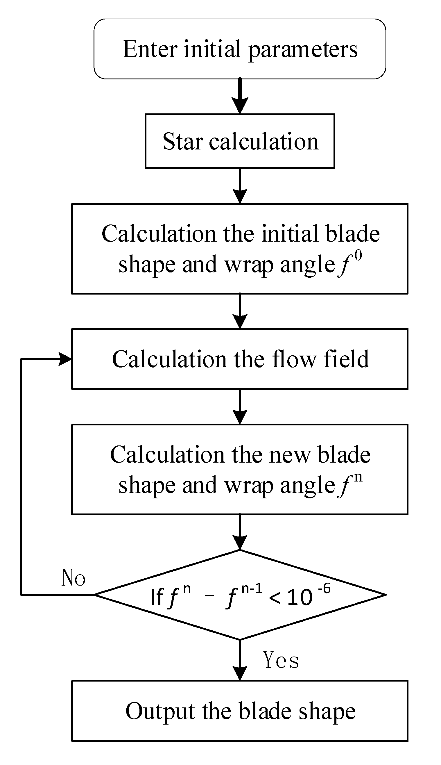
Once
and other design parameters were known, the blade shape and corresponding flow field can be calculated as shown in
Figure 4. The pressure distribution at the blade surface and the blade shape [
9] can be calculated by Equations (3) and (4) respectively.
where
is the static pressure at the blade work surface;
is the static pressure at the blade suction surface;
is the fluid density;
is the relative velocity on the blade surface;
represents streamline in the meridional shape and
means at the blade leading edge,
means at blade trailing edge.
and
are the axial and radial components of the circumferential average absolute velocity, respectively;
,
, and
are the axial, radial and circumferential components of periodic velocity, respectively;
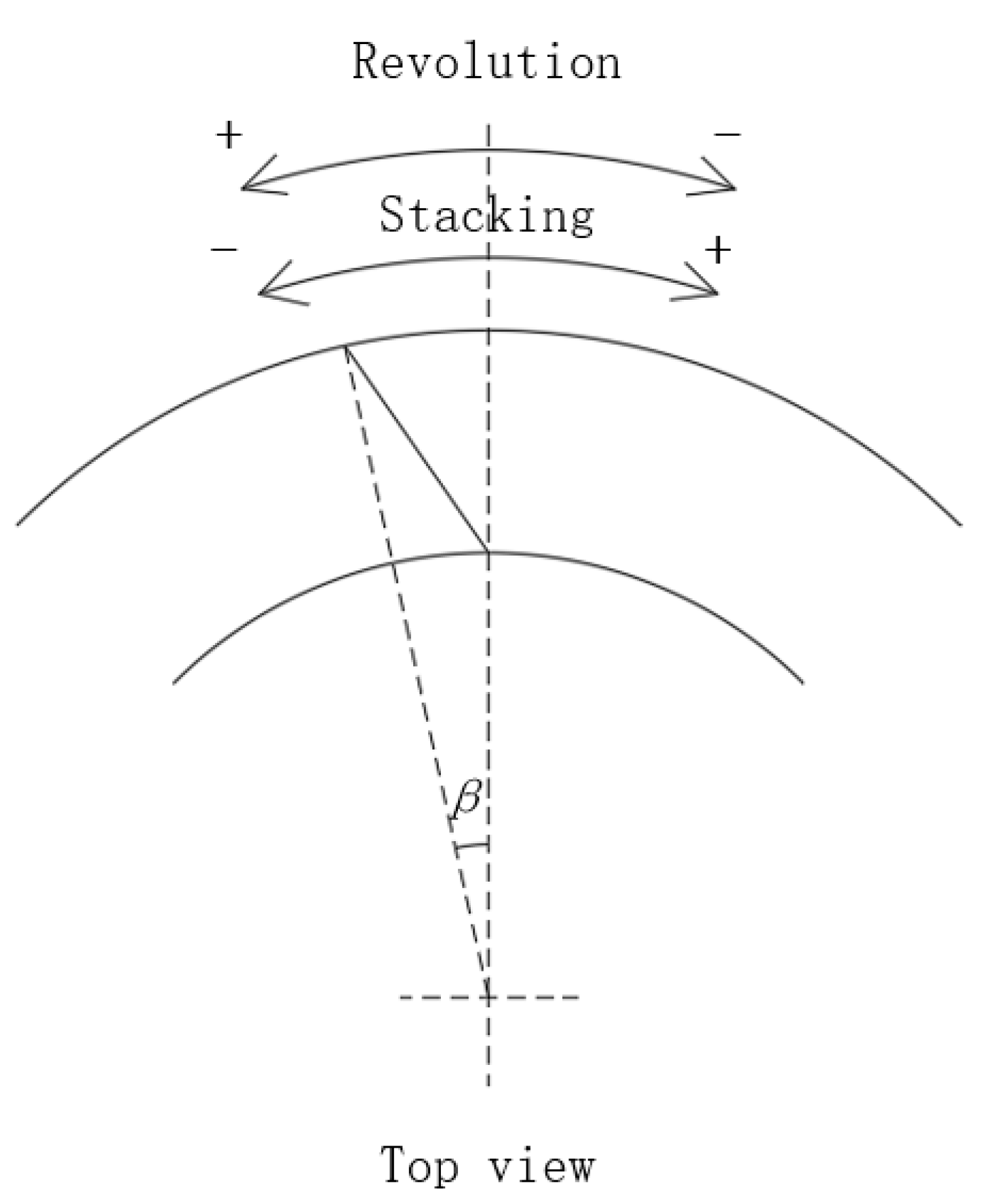
is wrap angle and can be calculated through integration along the streamline, the initial wrap angle
was prescribed by stacking condition which could specify the blade lean at trailing edge as shown in
Figure 5.
To obtain the impeller model, the following parameters need to be provided.
Design specifications and fluid properties.
Meridional shape.
Spanwise distribution of at the impeller exit.
The meridional derivative of the circulation (blade loading) at the hub and shroud.
Stacking condition.
3.3. Optimization Process
Construction of the approximate function between the design parameters and optimization objective is important in the optimization process. In this study, the approximate function is established by RSM using the second-order polynomial:
where
is the number of design parameters;
,
,
and
are the polynomial coefficients and can be determined by the least square method with the help of database sample points which create by DOE.
For DOE, the LHS method was used to construct the database sample points. This method can approximate random sampling from multivariate parameter distribution [
25]. First, it divides the sampling unit into different layers according to a certain characteristic or a certain rule, and then draws samples independently and randomly from different layers. Therefore, the structure of the sample is similar to the overall structure, so that a small number of sample points can be used to construct an accurate approximate function between the design parameter and the optimization objective in the entire design space.
NSGA-Ⅱ [
26,
27] was used for multi-objective global optimization. Every optimization objective was treated separately in NSGA-Ⅱ. “Mutation” and “crossover” were used to ensure that the final result is the global optimal solution. “Crowding distance sorting” and “non-dominated sorting” were used to reduce the process complexity and improve the elitism of the strategy.
All the above mentioned softwares are integrated on the Isight 5.8 platform to automatically execute the optimization process. Firstly, select appropriate design parameters and their ranges from IDM according to the optimization objectives. Secondly, use LHS to construct a proper number of different design parameters combinations in the entire design space as database sample points. Thirdly, use the different design parameter combinations from the second step to generate different impeller through IDM and use ANSYS CFX to calculate the impeller performance. Furthermore, RSM is used to construct the approximate function between the design parameters and optimization objectives. In this step, using ANSYS CFX to calculate impeller performance requires enough time and high computing resources, especially when the database sample point is large. Finally, NSGA-Ⅱ is used to solve the approximate model to obtain the Pareto optimal solution set.
4. Optimization Settings
4.1. Design Parameters
It can be seen from the introduction of the IDM that the distribution of and stacking conditions are closely related to the blade shape and the pressure distribution. Therefore, the distribution of along spanwise at the impeller exit, the distribution of blade loading along meridional shape at hub and shroud, and stacking were selected to parameterize the impeller, other parameters keep unchanged during the optimization process.
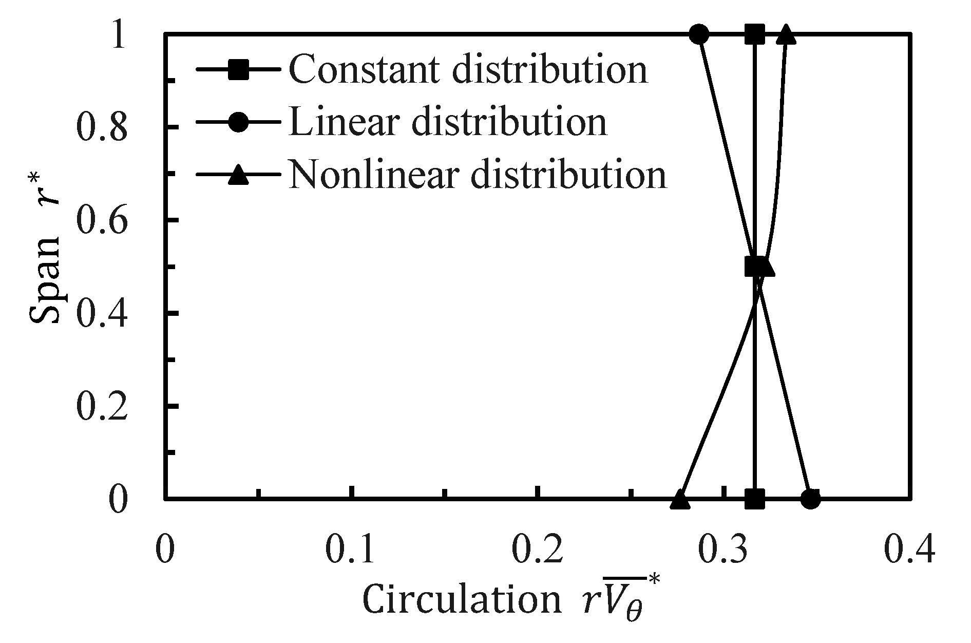
In this study, the second-order parabolic was chosen to describe the SDIEC.
where
,
, and
are the undetermined coefficients.
To determine the values of , , and , the value of at three different points in the spanwise of the impeller exit needs to be known. In this study, the value of (the value of at hub) and (the value of at shroud) are selected as design parameters. The value of at mid-span is automatically determined according to the impeller Euler head. When the values at these three points are determined, the values of , , and can be calculated. Thus, the unique second-order parabolic equation is established and all the values at other positions of the spanwise can be determined.
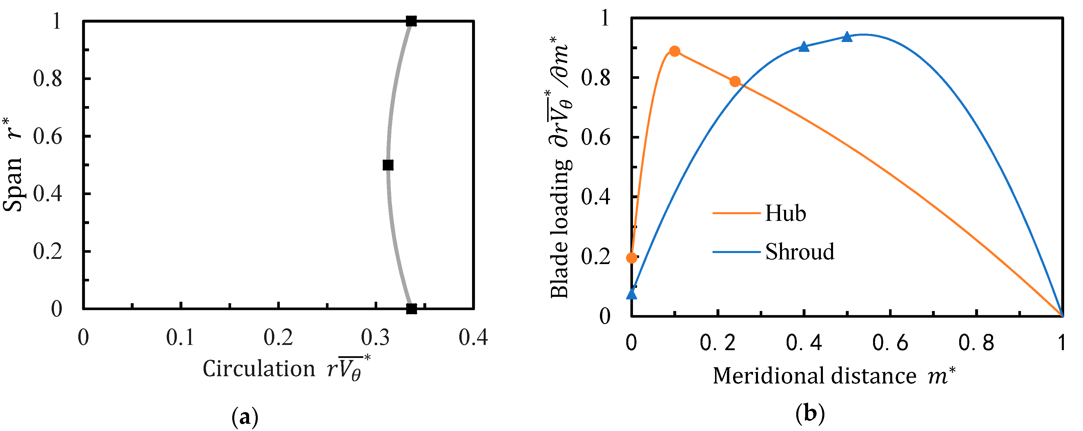
Three different
distribution forms at impeller exit are shown in
Figure 6, in this figure,
is the normalized spanwise distance at impeller exit and
is the normalized circulation.
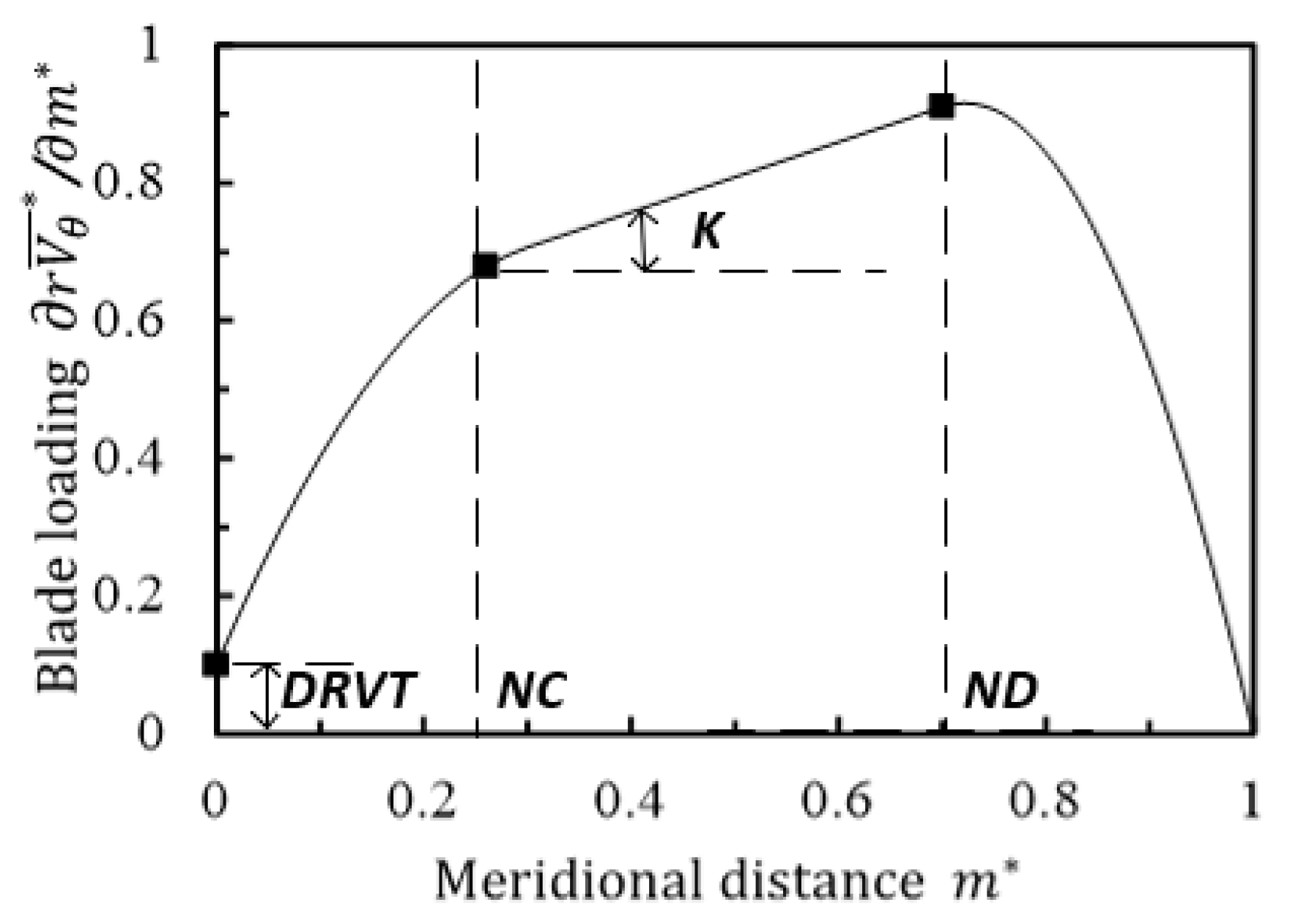
The distribution of blade loading along meridional shape at hub and shroud is a typical “three-segment” distribution as shown in
Figure 7, where
is the normalized meridional distance. For each streamline, the distribution of blade loading is determined by the following four parameters,
DRVT,
K, NC, and
ND. DRVT and
K represent the blade loading at the leading edge and the slope of linear line respectively.
NC and
ND are the locations of the connection points between the parabolic curve and the straight line. The blade loading at other positions between hub and shroud were determined by linear interpolation.
For mixed-flow pump design, stacking condition is also an important parameter since it can effectively suppress the generation of secondary flow [
28,
29]. Generally, the stacking
is considered negative if the blade leaned against the rotation direction as shown in
Figure 5. With this condition, the pressure at the hub will increase and the pressure at the shroud will decrease.
Therefore, the parameterization of the impeller can be completed by the following eleven parameters:, , , , , , , , , , and .
4.2. Optimization Objectives and Constraints
To improve the performance of the mixed-flow pump, the pump efficiency
at 0.8
Qdes and 1.2
Qdes were selected as the optimization objectives to enlarge the operating range of the high efficiency area. To make the optimized pump have similar specific speed, higher pump efficiency and better cavitation performance at the design point, the pump head
, efficiency
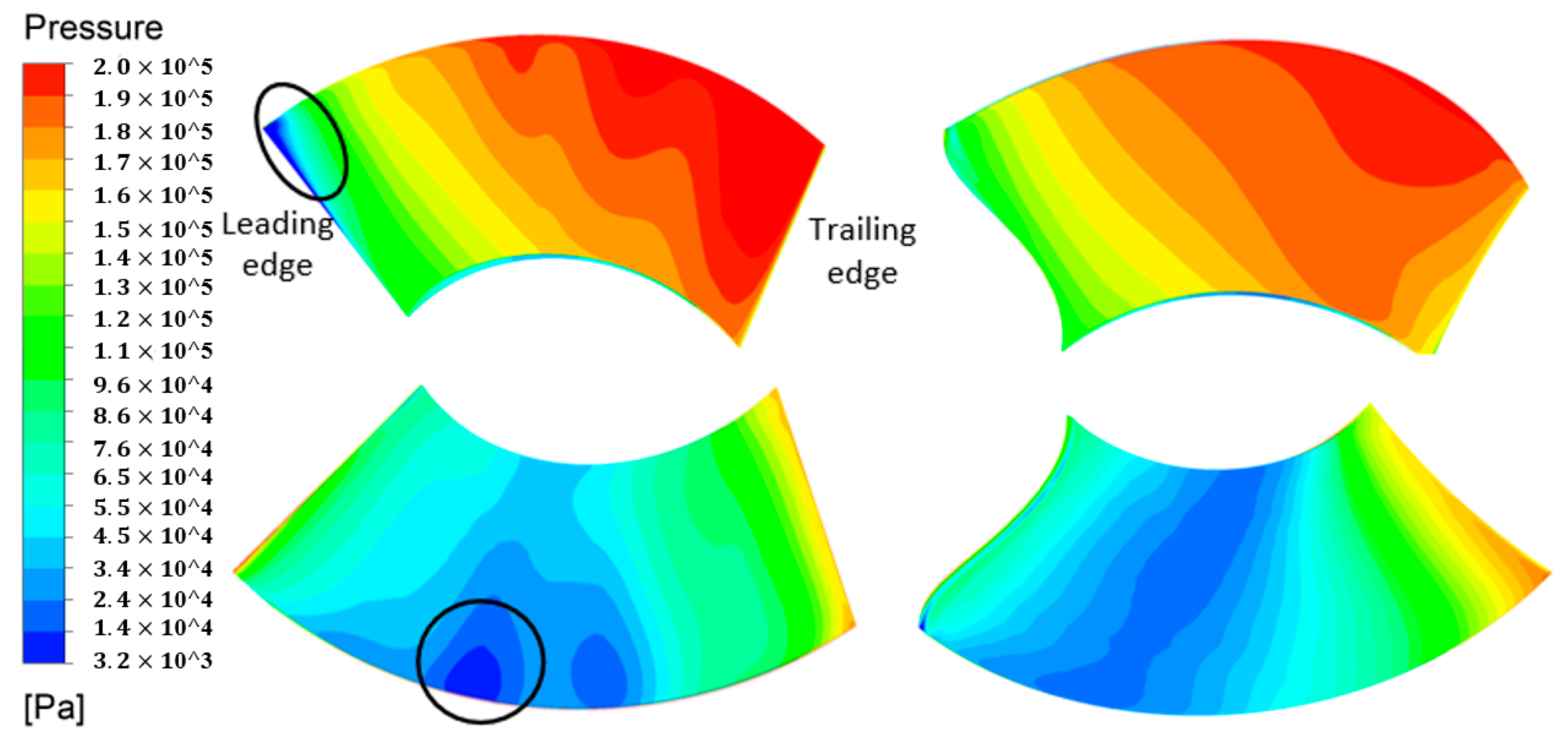
and the normalized area of low-pressure area
(the area on the blade surface where pressure is lower than water vaporization pressure 3169 Pa) at 1.0
Qdes were selected as the constrains. The optimization objective can be calculated by Equation (7), the constrains can be described as Equations (8)–(10):
where
and
are the total pressures at outlet and inlet, respectively;
is the torque on the impeller;
is the angular velocity of the impeller;
is the density of the fluid;
is the gravitational acceleration;
is the head of the original model at the design point;
is the pump efficiency of the original model at the design point;
is the low-pressure area of the original model at the design point,
is the low-pressure area of the optimized model at the design point.
4.3. Algorithm Settings
The number of design parameters
N is one of the important factors that affect the accuracy of the approximated model. Generally, the number of design parameters should be less than ten [
30]. After a great number of impeller generation and performance verification, the two parameters
and
with the least influence on performance were found and fixed at 0.1 and 0.4 respectively. The remaining nine parameters and ranges are shown in
Table 3, and all selected as design parameters.
The other important factor is the number of sampling points. From Equation (5), the least number of sampling points is , however, to make RSM more accurate, the recommended sampling points is twice the number of least sampling points. In this study, is 9, hence, 140 sampling points were generated by using LHS. Among those sample points, 110 sampling points were used to construct the approximated model and 30 sampling points were used for error analyses.
The settings of NSGA-Ⅱ are shown in
Table 4. Generally, too small “population size” will lead to difficulty in obtaining the optimal solution, and too large “population size” will result in a slower convergence rate, therefore, the recommended value is between 30 and 160 [
31]. The “population size” and “number of generations” are both in the present study are set to 100 with a total of 10,000 different configurations of impellers generated in this step.
6. Conclusions
In this study, a mixed-flow pump which is presently used in the South-to-North Water Diversion Project is optimized using a combined optimization system. The impeller was parameterized by IDM, and the circulation, blade loading, and stacking were selected as the design parameters. The pump efficiency at 0.8Qdes and 1.2Qdes were selected as the optimization objectives while the head, efficiency and area of low-pressure area at 1.0Qdes were selected as constraints. The results of this study can be summarized as follows:
- (1)
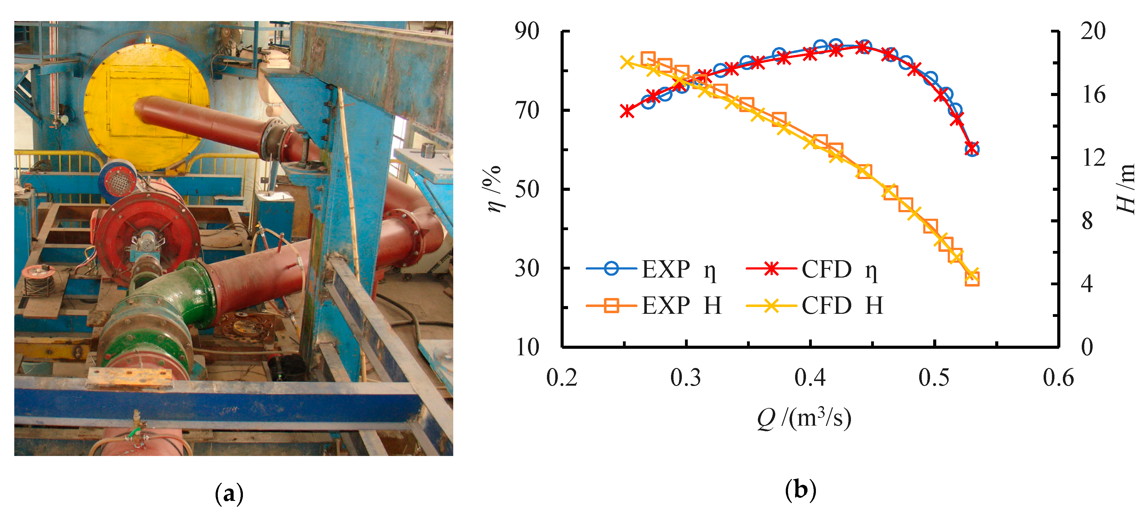
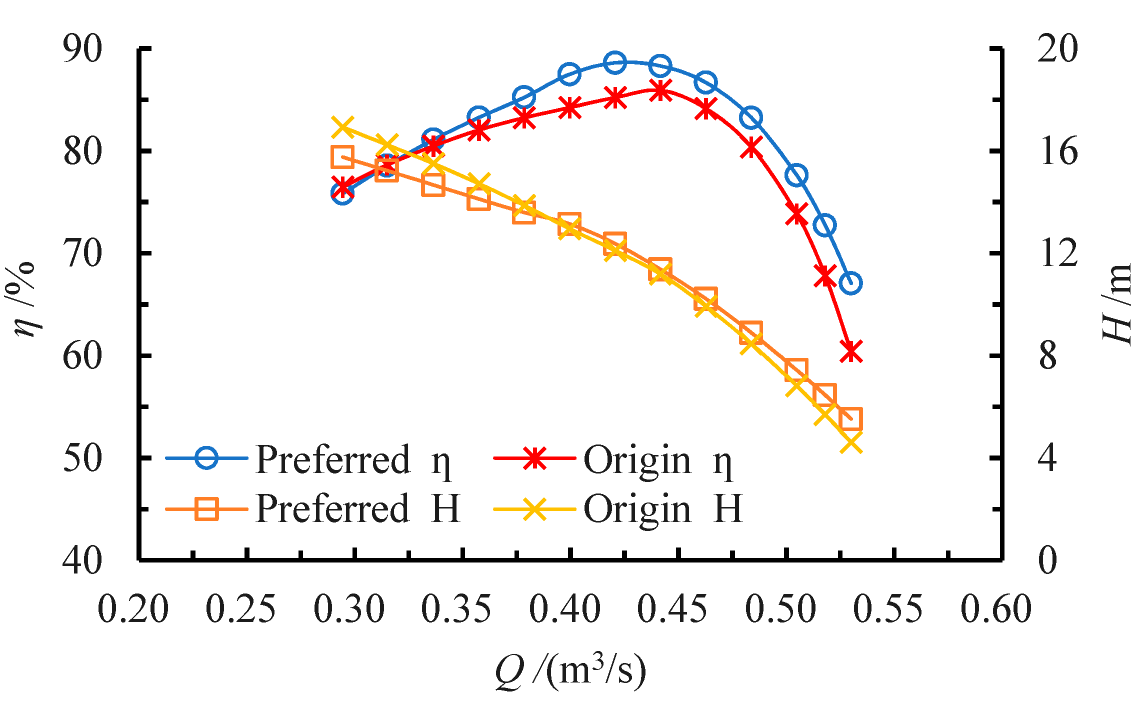
The CFD calculations accurately simulated the flow in the pump, and the performance curves agreed well with the experimental curves. The maximum efficiency and head deviations did not exceed 2% and 4% respectively.
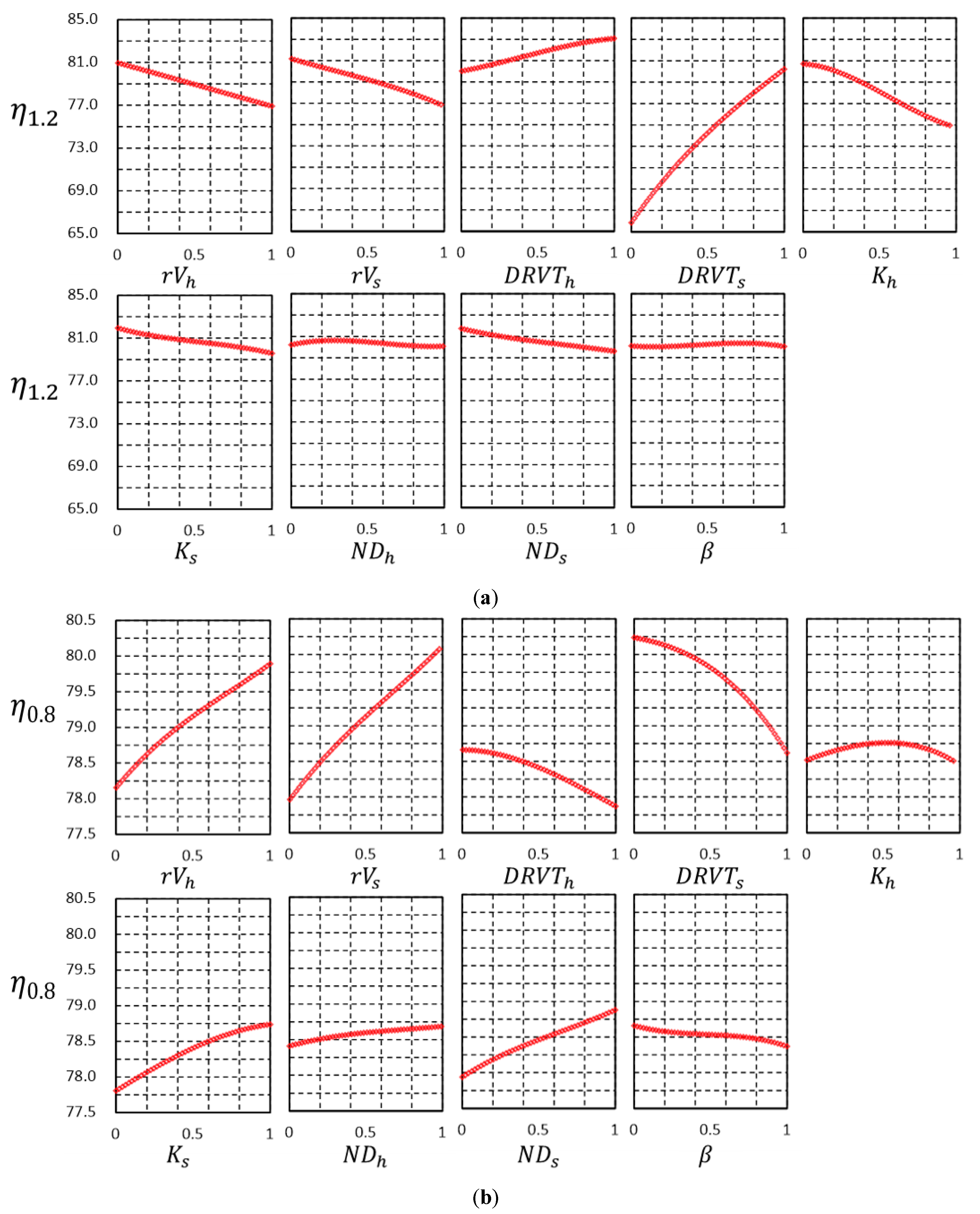
- (2)
The optimization results show that the non-linear SDIEC is better than the constant and linear distributions. The analysis of the main effect also shows that and have a greater impact on the performance of the mixed-flow pump impeller than other design parameters. Therefore, it is necessary to take and as design parameters in the optimization process to further improve the performance of the mixed-flow pump impeller.
- (3)
The pump efficiency with preferred impeller at 0.8Qdes, 1.0Qdes, and 1.2Qdes are 81.11%, 88.60%, and 77.62%, respectively. Compared with the original model, these efficiencies increased by 0.63%, 3.39%, and 3.77%, respectively. At the same time, the cavitation performance of preferred impeller has been significantly improved. The area of low-pressure region further reduced by 96.92% and the pump head deviation at 1.0Qdes is less than 1.84%, which is within an acceptable range.
Therefore, the design method proposed in this paper can reliably and effectively improve the comprehensive performance of the mixed-flow pump under the premise of small head changes.


