Valuation of the Energy Performance of a Greenhouse with an Electric Heater Using Numerical Simulations

Abstract

In Mexico, there are regions where the temperature drops below the minimum threshold for tomato cultivation (10 °C), requiring the implementation of auxiliary equipment to heat greenhouse air. The objective of this work was to estimate the energy consumption necessary to maintain climate requirements of a greenhouse located in Texcoco, State of Mexico, by using a model of energy balance implemented on Computational Fluid Dynamics (CFD) simulations. The temperature prediction relied on a numerical model based on CFD, proposing a benchmarking on the position and direction of the heater to estimate its effect on the thermal distribution. Results indicated that heater operation on January 2019, a power of 85.56 kW was needed to keep the greenhouse at 12 °C. Also, simulations indicated that electric heater used was not enough to get a homogeneous temperature inside the greenhouse. To achieve well-distributed thermal conditions, it was necessary to consider both the direction and position of heaters. Consequently, airflow direction became more important than height of the heater in order to homogenize the greenhouse area, given that the thermal gradient was reduced due to reverse heat flows.

1. Introduction

Plant growth greatly depends on the temperature and humidity. For winter production in Central Mexico, greenhouses provide better environmental conditions for plant growth compared to most agricultural production systems. Given that a greenhouse is a structure favoring environment for crop production, there are consequences such as heat excess during the day is absorbed by the ground and during the night it is used to meet the heating needs in enclosed greenhouses [1]. In this way, one of the characteristics of enclosed greenhouses is that they are energy saving compared to greenhouses fully relying on natural ventilation. However, accumulation of energy during the day may become insufficient [2] with higher frequency during the winter. Therefore, night temperature becomes a critical factor in the efficiency of a crop cultivated in a greenhouse. Adequate greenhouse energy management can serve to avoid low night temperatures and reduce condensation phenomena causing dripping process on crops [3,4,5,6].

A conventional solution for low-temperature problems is using heating systems inside the greenhouse. Since energy and fuel prices are not cheap [7], their efficient use directly impacts production costs and should be balanced with the risks of crop loss [8,9]. Nonetheless, the amount of heat added to the greenhouse depends on the changing weather conditions, where winter becomes the critical period [10]. Previous research [10,11] have stated that more attention should be given to the night due to significant heat losses, which should be compensated by means of an artificial heat input.

In addition to conventional heating systems (fossil fuels), there are alternative systems used to heat the interiors of greenhouses, among which are renewable energy source systems. These systems allow the use of biomass, solar, and geothermal energy sources [12,13,14,15,16,17], with solar energy being the most recommendable, given that it is a clean, abundant, and safe source. One of the greenhouse heating systems that uses solar energy as a main source and that has been studied by many researchers is rock bed storage. This type of system uses underground rocks to store heat during the day and release it at night, generating an increase in air temperature of up to 3 °C, causing improvement of fruit quality by up to 29% [18,19].

In some greenhouse production systems, the energy consumption represents more than 50% of the total cost of production, and it is necessary to calculate its consumption. The more accurate approach is employing mathematical models based on the principle of heat and mass conservation in order to estimate the feasibility of the implementation of control systems during the winter. Numerical models are also used to improve the understanding of convective, radioactive, and conductive phenomena and the environment-plant iteration within the greenhouse [20,21,22,23]. These findings have allowed us to deepen our understanding of the dynamics of the microclimate and the energy needed to maintain environmental comfort, achieve a high-performance production, and improve the quality and efficiency of heating systems [24,25,26].

Modeling by means of Computational Fluid Dynamics (CFD) has achieved an approach to simulate air movement and temperature variation within the greenhouse and the impact of heating systems on the thermal gradient [27,28,29,30,31,32]. Along with this, it has allowed us to refine sub-systems of the greenhouse such as the heating system to increase its effectiveness and efficiency. Some studies carried out in CFD have allowed us to establish that, by using heating pipes, it was possible to increase the temperature inside the greenhouse by up to 4.5 °C [11]. In 2018, Yilmaz and Selbas [33] investigated the thermal performance of a solar collector, a heat pump, and a boiler for heating a greenhouse. The results showed that the solar collector had a greater impact on the thermal gradient of the greenhouse, with a thermal efficiency of 33.11%. Another work in 2017, Tadj et al. [27] demonstrated that perforated polyethylene duct heating systems generated a uniform temperature compared to other heating systems (hot water pipes and air heaters). These results agreed with what was established in the literature, in which the temperature distribution was more homogeneous in a vertical plane than in a horizontal plane [34].

In regions with mild winters and at specific periods of the year, an emergent heating system is being needed to mitigate occasional frosts. In central Mexico, it is common to place pop-up heaters aiding to stabilize the internal temperature when the outside temperature drops abruptly in specific hours before sunrise. Even though empirical experience has been gained, there is still scarce research about optimal use of electrical heating systems. For instance, recommendations about the position and direction of heaters to optimize amounts of heat that guarantees thermal homogeneity during these critical periods. Nor it is found related research on the energy and economic costs of this emerging heating system.

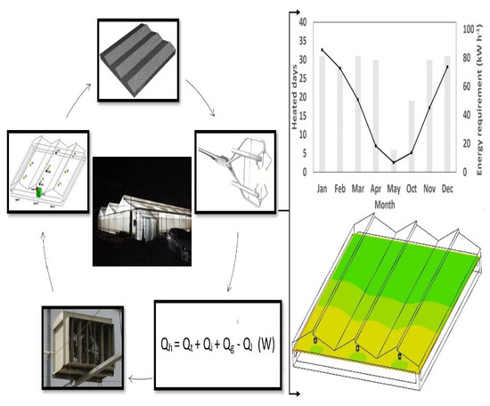
Then, the aim of this work was to estimate the necessary energy consumption to maintain thermal homogeneity using an electric heater in the greenhouse under winter conditions in central Mexico, using a model of energy balance and CFD to predict the thermal distribution under different heating scenarios.

2. Materials and Methods

2.1. Experimental Ground Description

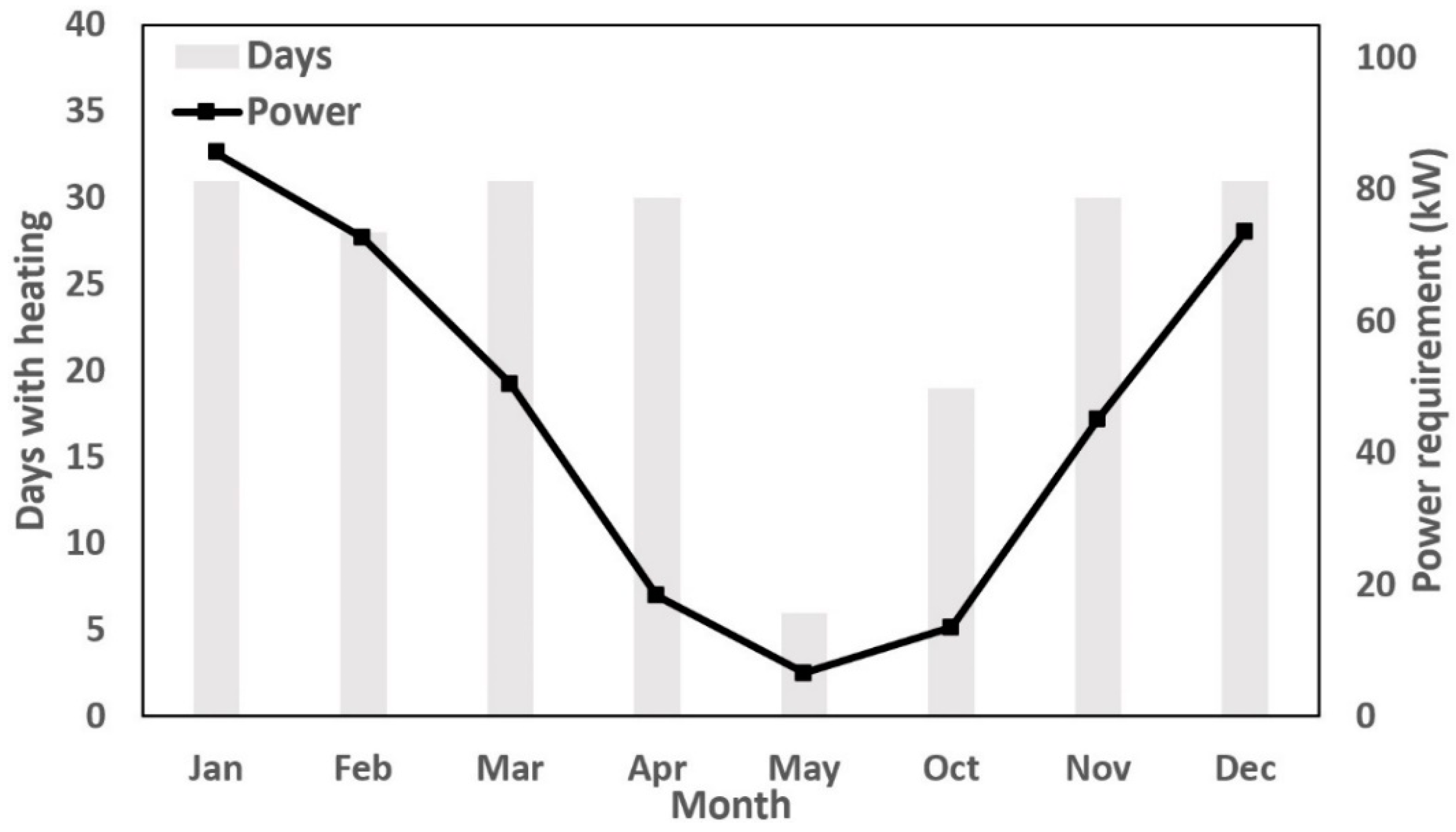
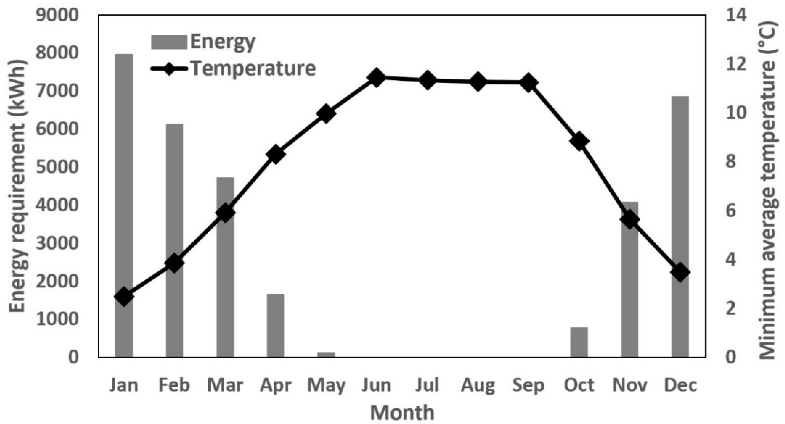
The site of the experimental greenhouse was located at Campus Graduate College in the State of Mexico (19°27′45.5″ N, 98°54′12.2″ W) at 2239 masl, situated on flat ground with no structures around it. In the region, the minimum monthly temperatures range between 2.49 °C and 11.24 °C throughout the year.

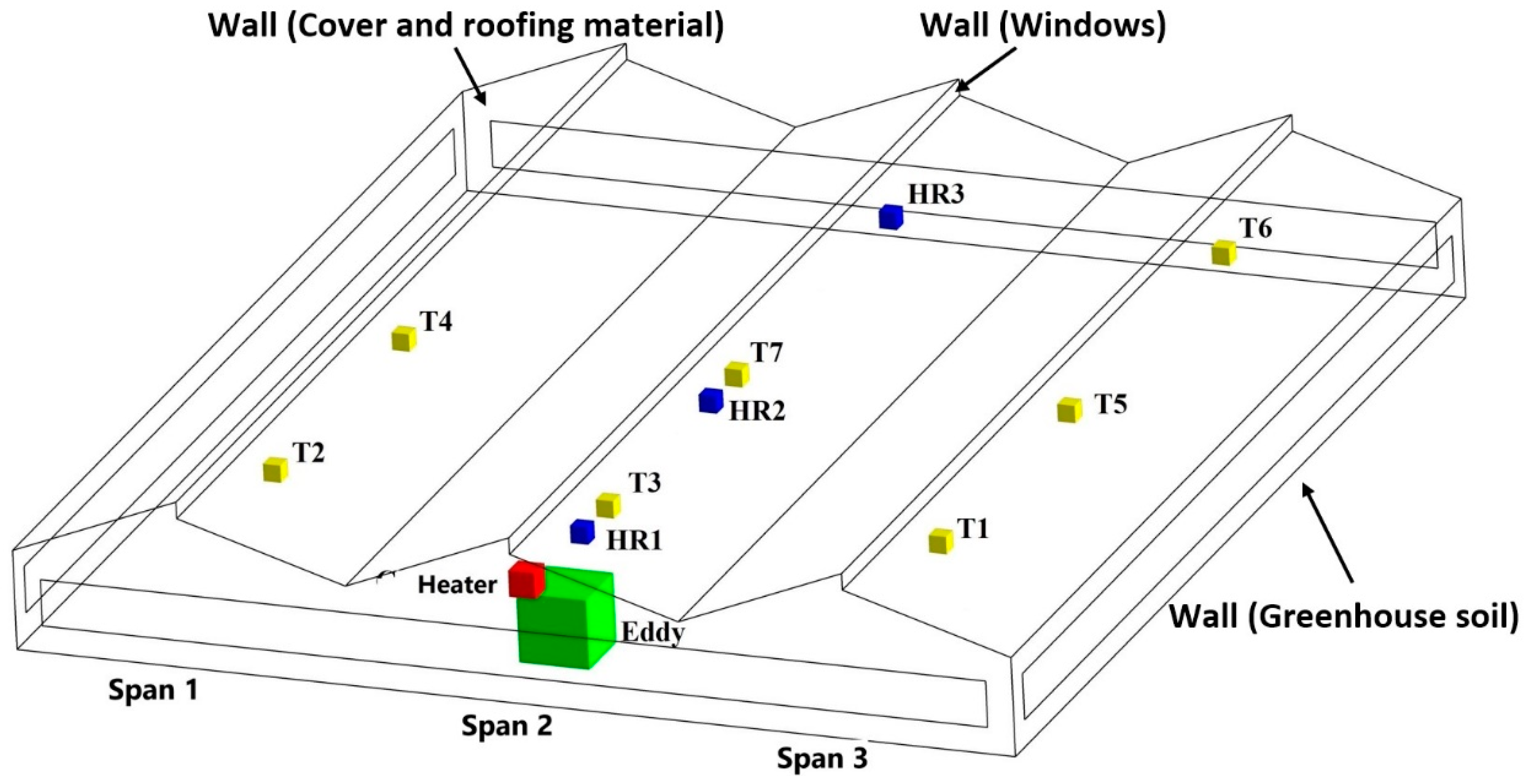
The prototype greenhouse had an area of 1050 m². It was of the zenith type with three spans covered with translucent polyethylene on the floor and sides, polycarbonate on the roof, and anti-insect on the windows. The greenhouse had a natural ventilation system based on the closure and opening of the overhead and front windows and a heating system using an electric heater (CM-VAX, Calelec, Monterrey, Mexico) recommended for enclosed spaces with an area of 96 m². The electric heater was located 3 m above the ground level in span 2 in the windward zone and had a power of 15 kW. Its electrical characteristics were 230/3/60 (Volts/Phases/Cycles), and it had an axial fan with a motor of 1/8 HP that worked with 120 V.

For data acquisition, an Eddy Covariance system 2.4 m away from the windward position with a sonic anemometer (CSAT 3D, Campbell Scientific Ltd., Antony, France), an EC150 gas analyzer (Campbell Scientific Inc., Logan, UT, USA), a temperature and humidity sensor (HMP155A, Campbell Scientific Logan, UT, USA) and four sensors for soil temperature (TCAV thermocouple Campbell Scientific Logan, UT, USA) which were placed inside the greenhouse. Seven temperature sensors (DS18B20, Maxim Integrated, San Jose, CA, USA) and three relative humidity sensors (DHT22, Zhengxinyuan Electronics Co., Ltd., Shenzhen, China) were distributed in the three spans at a height of 3 m (Figure 1).

Data recording and storage were performed every 5 s for the temperature and humidity and every 100 ms for the anemometer. The monitoring period was from February 3 to February 24, 2019, which was enough time to investigate the emergent heater, since the meteorological data recorded minimum temperatures during this month of below 12 °C. The data was stored with a data logger system (CR3000 Micrologger, Campbell Scientific, Inc., Logan, UT, USA) for the Eddy Covariance system and an Arduino data Logger Shield for the DS18B20 and DHT22 sensors. Outside the greenhouse, a weather station (Vantage Pro2 Plus, Davis Instruments, Hayward, CA, USA) was available and used to record data on temperature, humidity, wind direction, and wind speed—these values were used as the initial boundary condition of the computer model. All data was processed in Microsoft Excel to determine the environmental input conditions of the computational model.

2.2. Heat Calculation

The greenhouse temperature model was developed based on the energy and mass balances [24,25,35,36] in the completely closed greenhouse without environment-plant iteration, because at the time of data recording there was no crop. The calculation of Q_h was estimated by establishing the necessary energy consumption transferred by the electric heater to attenuate the thermal gradient, expressed as follows:

$$Q_h=Q_t+Q_i+Q_g-Q_l \left(\mathrm{W}\right).$$

(1)

The thermal radiation transferred from the inside to the outside of the greenhouse ($Q_l$) depended on the emission of energy into the atmosphere and on the roofing materials.

$$Q_l=S_{sc}·\sigma ·{\tau }_{ter}·\left({\epsilon }_{atm}·T_{atm}^4-{\epsilon }_{ter}·T_c^4\right) \left(\mathrm{W}\right),$$

(2)

where S_sc is the floor area covered (m²), $\sigma$ is the Stefan–Boltzmann constant (W m⁻² K⁻⁴), ${\tau }_{ter}$ is the transmittance coefficient of the cover material for thermal radiation, ${\epsilon }_{atm}$ is the emissivity of the atmosphere, T_atm is the temperature of the emission of energy to the atmosphere (K), ${\epsilon }_{ter}$ is the emissivity of the roofing material for thermal radiation, and T_c is the absolute temperature of the roof (K).

The heat transfer by conduction and convection (Q_t) was estimated by the temperature between the inside and outside of the greenhouse.

$$Q_t=S_{dc}·K_{cc}\left(t_i-t_e\right) \left(\mathrm{W}\right),$$

(3)

where S_dc is the developed area of the greenhouse cover (m²), t_i is the interior temperature of the greenhouse (K), t_e is the exterior temperature of the greenhouse (K), and k_cc is the overall coefficient of heat loss by conduction and convection (W m⁻² K⁻¹).

The sensitive and latent heat lost by the renewal of indoor air (Q_i) was considered minimal when establishing as an initial condition the closing of the side and overhead windows. However, there is air infiltration through the structure as it is an old construction becoming a partially airtight greenhouse.

$$Q_i=V_{gh}·\frac{R}{3600}·\rho ·\left[c_{pa}·\left(t_i-t_e\right)+{\lambda }_0·\left(x_i-x_e\right)+c_{pv}·\left(x_i{t}_i-x_e{t}_e\right)\right] (\mathrm{W}),$$

(4)

where V_gh is the volume of the greenhouse (m³), c_pa is the specific heat of the air (J kg⁻¹ K⁻¹), $\rho$ is the density of the air (kg m⁻³), c_pv is the specific heat of the superheated steam (J kg⁻¹ K⁻¹), x_i x_e is the absolute indoor and outdoor humidity (kg kg⁻¹), ${\lambda }_0$ is the latent heat of vaporization (J kg⁻¹), and R is the air renewal rate (h⁻¹).

The heat transfer through the ground (Q_g) is a function of the difference in the indoor and soil temperature.

$$Q_g=K_{ts}·S_{sc}\frac{\left(t_i-t_s\right)}{p} (\mathrm{W}),$$

(5)

where K_ts is the coefficient of thermal exchange through the soil (W m⁻¹ K⁻¹), t_s is the soil temperature (K), and p is the depth at which the temperature is estimated (m).

The parameters of the energy balance model were analyzed considering the effect of the greenhouse environment, its characteristics, and the roof materials (

Table 1. Variables for the heat calculation obtained from the literature.

Symbol	Variable	Value	Unit	Source
σ	Stefan–Boltzmann constant	5.67 × 10−0.8	W m−2 K−4	[37]
α	Polycarbonate absorbency	0.09		[37,38]
τter	Transmittance coefficient of the polycarbonate	0.025		[37,38]
εter	Polycarbonate emissivity	0.935		[37,38]
Cpa	Specific heat of the air	1008	J kg−1 K−1	[24,25]
R	Air renewal rate	4	h−1	[39]

and

Table 2. Characteristics of the greenhouse and its components.

Symbol	Variable	Value	Unit
Sdc	The developed area of the greenhouse cover	1113	m2
Ssc	Floor area covered	1050	m2
ec1	Polycarbonate thickness	0.06	m
ec2	Polyethylene thickness	0.000018	m
Vgh	Greenhouse volume	4,068,076	m3

).

The heat calculation was made using the average weather condition rates of minimum daily temperature. Inside temperature of the greenhouse was established as 12 °C based on the thermal requirement of the tomato (Solanum Lycopersicum L.), which, for proper growth, the temperature should be higher than 10 °C at night [40,41].

2.3. Computational Model

Building and simulation of the computational model was carried out in ANSYS^® Fluent^® (ANSYS, Inc., Canonsburg, PA, USA). The geometry was developed in the design modeler tool. The meshing was done in meshing, and the greenhouse had dimensions of 30 × 35 × 5 m, with 490,000 average structured elements, an orthogonal quality of 0.98, and a distortion of 1.935 × 10^−0.02.

Model conditions and variables applied to the airflow to solve the transport equations, which were discretized into algebraic equations and calculated by numerical methods, were defined in

Table 3. Boundary conditions of the computational model.

Boundary Condition	Method
Solver	Pressure-based
State	Steady
Viscosity function	k-ε Estándar
Energy equation	Activated
Entry	Velocity inlet
Output	Pressure outlet
Air temperature	Constant (12.73 °C)
Wind speed	Constant (0.513 m s−1)
Heat source	Boussinesq’s hypothesis
Soil thermal condition	Temperature (4.7 °C)
Soil	Wall (ρ:1300, Cp:800, λ:1)
Walls and greenhouse padding (Polyethylene PE)	Wall (ρ:925.5, Cp:1900, λ:0.3)
Ceiling (Polycarbonate PC)	Wall (ρ:1200, Cp:1200, λ:0.19)

.

Heater simulation included a pressure jump and angular velocity. The pressure jump calculation was estimated considering Equation (6):

$$\Delta p=\frac{1}{2}{\rho }_{air}{v}^2 (\mathrm{Pa}),$$

(6)

where ${\rho }_{air}$ is the air density (kg m⁻³) and $v$ is the fan speed (m s⁻¹).

Evaluation of the Computational Models

In order to obtain a reliable computational model, two scenarios were assessed: (I) no heat and (II) with heat. The evaluation was carried out by a statistical analysis of both temperature and wind speed using simulated and experimental data. The statistic studios were made by an analysis of variance (ANOVA), with a significance level of 0.05 used to contrast the difference of the variables in the different factors parametrically.

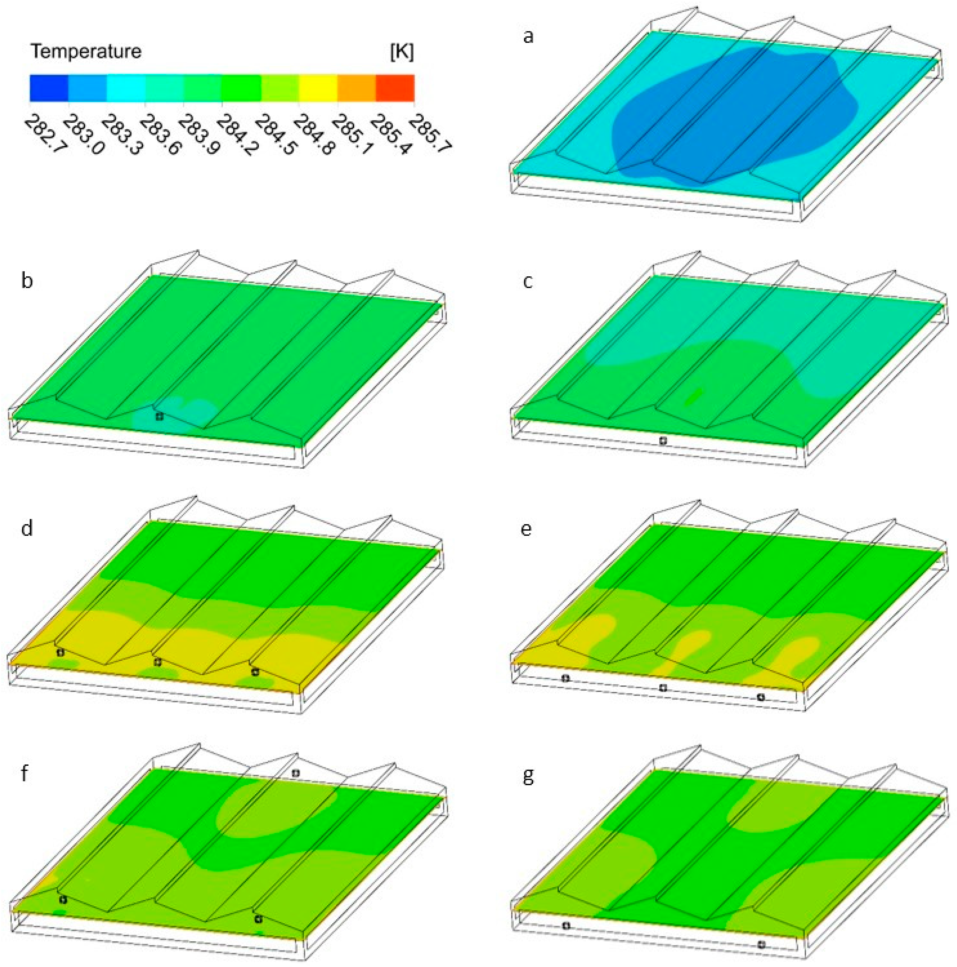
2.4. Simulation Scenarios

The analysis of the distribution of heat flow in the greenhouse was performed by comparing the effect of the position and direction of the heaters; two more heaters were included in the computational model, seeking to improve the system with a uniform temperature (

Table 4. Simulation scenarios (X transversal, Z longitudinal, Y height).

Sceneries	Heaters	Ubication in Greenhouse (Local Coordinates)	Heater Flow Direction
a	0
b	1	Span 2 (X: 0 m, Y: 3 m, Z: −16.5 m)	Z
c	1	Span 2 (X: 0 m, Y: 0.5 m, Z: −16.5 m)	Z
d	3	Span 1 (X: −10 m, Y: 3 m, Z: −16.5 m)	Z
		Span 2 (X: 0 m, Y: 3 m, Z: −16.5 m)	Z
		Span 3 (X: 10 m, Y: 3 m, Z: −16.5 m)	Z
e	3	Span 1 (X: −10 m, Y: 0.5 m, Z: −16.5 m)	Z
		Span 2 (X: 0 m, Y: 0.5 m, Z: −16.5 m)	Z
		Span 3 (X: 10 m, Y: 0.5 m, Z: −16.5 m)	Z
f	3	Span 1 (X: −10 m, Y: 3 m, Z: −16.5 m)	Z
		Span 2 (X: 0 m, Y: 3 m, Z: 16.5 m)	−Z
		Span 3 (X: 10 m, Y: 3 m, Z: −16.5 m)	Z
g	3	Span 1 (X: −10 m, Y: 0.5 m, Z: −16.5 m)	Z
		Span 2 (X: 0 m, Y: 0.5 m, Z: 16.5 m)	−Z
		Span 3 (X: 10 m, Y: 0.5 m, Z: −16.5 m)	Z

). Simulations were carried out in a stationary state, and the provided energy was modified by the heater based on the assessed computational model’s results. The origin of the coordinates (x, y, z) is in the center of the greenhouse, and the flow direction of the evaluated heater is z.

3. Results and Discussion

3.1. Energy Consumption

Figure 2 shows the estimation of the necessary heating days and their average power requirement. For their calculation, the results obtained from Equation (1) were used, considering that power requirement is required on days with a temperature below 12 °C inside the greenhouse. The monthly power requirement is the arithmetic average of the air conditioning calculation of the days with heating needs during the year.

Results from Figure 2 show that, during certain hours at night, is necessary to heat the greenhouse’s air for 206 days. January was the month with the highest energy requirement, needing an implementation of five more heaters with the same conditions to cover the energy needs and maintain a 12 °C temperature. This means that for thermal comfort in the microclimate of the greenhouse, a device providing 85.56 kW is required.

In Figure 3, a comparison was made between the average minimum monthly temperature in the study area and the energy required to maintain the greenhouse at 12 °C (Equation (1)). The calculation of the monthly energy requirement was carried out by assuming that the period in which the temperature falls below 12 °C during the days with heating needs occurs for an average of three hours per day. The peak of the needs was produced in January and is 13.94% higher than the one in December. During the period from June to September, there is no energetic demand. To cover the annual demand, 32,228.76 kWh is necessary, which represents a cost of MX $20,626.40 (US $540.0) according to the nine tariff charges applied to the agriculture in Mexico.

3.2. Mesh Sensitivity Analysis of the Computational Model

A sensibility mesh analysis was carried out in the greenhouse by 100 temperature measurements in a location 2 m above the ground. Four scenarios were performed by modifying the number of elements of the inside mesh of the greenhouse. The results showed that there is no meaningful difference between the simulated temperature results with a 490,000 average element mesh.

3.2.1. Validation

The evaluation of the computational model with and without heating was carried out statistically by correlating the values of temperature and wind speed simulated and recorded by the sensors during the nights of February 6th and 7th, 2019, respectively. In

Table 5. Temperature data (°C) of the evaluated models.

Model without Heating			Heated Model
Sensor	Experimental	Simulated	Sensor	Experimental	Simulated
T1	11.28	11.42	T1	10.96	11.03
T2	10.28	11.43	T2	10.43	11.05
T3	10.95	11.3	T3	10.94	11.06
T4	10.93	11.33	T4	10.79	10.89
T5	11.52	11.31	T5	10.93	10.86
T6	11.5	11.4	T6	10.86	10.82
T7	11.31	11.29	T7	11.07	10.82
Eddy	11.76	11.85	Eddy	11.08	10.91

, it can be observed that the recorded and simulated temperature values were approximate. To measure this correlation, the statistical method ANOVA with a significance level of 0.05 was used, considering that if the F statistic test was less than the F critical value ( F test statistic < F critical value), there was no significant difference between the measured and simulated variables (

Table 6. Comparison between the F test statistic (ANOVA) and its critical value.

	With Heating	Without Heating
Temperature	0.3 < 4.6	1.62 < 4.6
Wind speed	0.005 < 7.7	3.25 < 7.7

), so the evaluated model can be used in simulations.

3.2.2. Environmental Analysis of the Assessed Model

An empty greenhouse was validated to give stability to the variables being analyzed. Once the model was validated, the crop could be modeled, since its thermal and relative humidity requirements were known. In some cases, tomato crop could be modeled as a source or sink of momentum, energy, and mass. The heatless model presented a thermic homogenization at 2 m high inside the three spans of the greenhouse. The speed was not superior to 0.018 m s⁻¹, and the number of Rayleigh (Ra) varied around 2.8 × 10⁸ for the three greenhouse’s spans, with a laminar flow induced by floating forces.

The computational model with heating shows that for span 2, there was an increase in the speed of wind generated by the fan (Figure 4). This rise in speed caused a low on span 2 near the windward. However, in the center of span 2, there was a rise of nearly 0.15 °C derived from the energy supply on the part of the heater.

On spans 1 and 3 of the model with heat prevailed the laminar flows induced by floating forces with Ra numbers between 4.09 × 10⁸ and 5.98 × 10⁸. On span 2 near the fan, the thermic distribution was in accordance with the speed and temperature provided by the heater, causing a transition zone in a turbulent flow (10 × 10⁸ to 10 × 10¹⁰) with Ra values of 2.42 × 10⁹.

These simulations presented a thermal behavior similar to the one obtained by Chen et al. [24], when greenhouses subjected to non-heating, laminar flows induced by prevailing buoyancy forces. And in greenhouses with heating, there was a turbulent flow transition.

3.3. Thermal Spatial Distribution of Simulated Scenarios

Figure 5 shows a top view of the temperatures at 2 m from the ground in the simulated scenarios with initial data from the computational model with and without heating. The results from the simulations present an increase in temperature of 0.8 °C between scenarios a and b, and an increase of 2 °C between scenarios a, d, and e.

Given that the maximum thermal gradient was 0.2 °C when the heater height was modified (Figure 5b–g), it was determined that if the direction of heat flow was the same, the height has no significant effect on the temperature’s distribution at 2 m from the ground under the original conditions of the heater. Unless the heat flow direction was changed (scenarios f and g), in this case, the homogeneity improved and the buoyancy forces had crucial importance in the heat distribution. The results of the simulations matched those presented in the works of Tadj et al. and Dhiman et al. [27,34], where the air heating was not the most efficient way in which to homogenize the greenhouse’s temperature on a horizontal level.

To review the results of Figure 5 and analyze the temperature behavior at 2 m from the ground and its influenced on the height and direction of the flow of the heater under different energy supplies, four scenarios were performed (d, e, f, and g) considering a constant supply of air with a temperature of 30 °C by the heater.

Figure 6 shows the relationship of the longitudinal temperature at 2 m high off the ground in span 2 between scenarios d and e (∆), with a constant temperature supply of 30 °C. The figure shows that if the direction of heat flow remained constant, there was no significant difference in the temperature at 2 m from the ground (R² = 0.996) between the heater at 0.5 and 3 m. However, this heater position was not adequate to homogenize the vertical temperatures longitudinally 2 m from the ground, since, as the energy provided by the heater increases, the thermal gradient was more significant between the area near the heater and its opposite side. Scenarios d and f (o) showed that in span 2, the direction of heat flow had a more significant impact on the distribution of horizontal temperatures at 2 m high, improving the homogenization and reducing the thermal gradient when mixed heat fluxes are present (scenario f).

Through the simulation results of this work, it was possible to assume that the direction of heat flow had a significant impact on thermal homogenization (scenarios d and g), reaffirming the work of Constantinos et al. [27], where the distribution of heat flow was caused by the position of the heating systems and the effect of floating forces created by the thermal gradient between the greenhouse temperature and the energy supplied by the heating system.

When selecting the location of the heater, it was necessary to take into account that the temperature was higher in the area near the heater, as shown in Figure 7. Therefore, to avoid crop damage, the heater must be installed at a height higher than the current crop. In the case of tomatoes, the recommended height was 3 m.

The power supplied by the greenhouse heater used in this research was insufficient to mitigate the temperature drop that occurs mainly during the winter period. In addition to the power, it was necessary to consider the distribution of electric heaters, since this type of system, compared to heating systems using pipe networks [34,42,43], was not the best option for homogenizing the temperature in the greenhouse. Currently, there are many techniques used to heat the air in the greenhouse [10,27,44]. However, due to the high investment cost of these systems, they sometimes become unfeasible.

4. Conclusions

During the winter in Central Mexico (December 21 to March 21), energy consumption is around 63% of the total for the year to maintain a temperature of up to 12 °C in the greenhouse during the night period. Such climatic conditions cause an approximate cost of MX $12,949.7 (US $540), according to the agricultural tariff in Mexico. Thermal distribution occurs in accordance with the speed and temperature provided by the heater, causing a zone with a turbulent flow and a difference in density between the air near the heater and the rest area of the greenhouse. Thermal homogenization in the greenhouse occurs when there are conditions for opposite heat flows (recirculation), causing an improvement in the greenhouse environment by the distribution of the heaters and reducing the temperature gradient between the area near the heater and its opposite side. This type of heater system, known as aerial, is not ideal for homogenizing the temperature of the greenhouse due to the effect of the buoyancy forces which can be overcome by adding fans at stagnant zones and aid to distribute the heat at all zones of the greenhouse.

References

1. Fidaros, D.K.; Baxevanou, C.A.; Bartzanas, T.; Kittas, C. Numerical simulation of thermal behavior of a ventilated arc greenhouse during a solar day. Renew. Energy 2010, 35, 1380–1386. [Google Scholar] [CrossRef]
2. Roy, J.C.; Pouillard, J.B.; Boulard, T.; Fatnassi, H.; Grisey, A. Experimental and CFD results on the CO2 distribution in a semi-closed greenhouse. Acta Hortic. 2014, 1037, 993–1000. [Google Scholar] [CrossRef]
3. Ali, H.B.; Bournet, P.E.; Danjou, V.; Morille, B.; Migeon, C. CFD simulations of the night-time condensation inside a closed glasshouse: Sensitivity analysis to outside external conditions, heating and glass properties. Biosyst. Eng. 2014, 127, 159–175. [Google Scholar] [CrossRef]
4. Salazar-Moreno, R.; Rojano-Aguilar, A.; López-Cruz, I.L. La eficiencia en el uso del agua en la agricultura controlada. Tecnol. Y Cienc. Del Agua 2014, 5, 177–183. [Google Scholar]
5. Salazar-Moreno, R.; Mauricio-Pérez, A.M.; López-Cruz, I.L.; Rojano-Aguilar, A. A model of humidity within a semi-closed greenhouse. Rev. Chapingo Ser. Hortic. 2016, 22, 27–43. [Google Scholar] [CrossRef]
6. Zeroual, S.; Bougoul, S.; Benmoussa, H. Effect of Radiative Heat Transfer and Boundary Conditions on the Airflow and Temperature Distribution Inside a Heated Tunnel Greenhouse. J. Appl. Mech. Tech. Phys. 2018, 59, 1008–1014. [Google Scholar] [CrossRef]
7. Tamimi, E.; Kacira, M. Analysis of climate uniformity in a naturally ventilated greenhouse equipped with high-pressure fogging system using computational fluid dynamics. Acta Hortic. 2013, 1008, 177–184. [Google Scholar] [CrossRef]
8. Bakker, J.C. Analysis of Humidity Effects on Growth and Production of Glasshouse Fruit Vegetables. Ph.D. Thesis, Agricultural University of Wageningen, Wageningen, The Netherlands, 1991. [Google Scholar]
9. Baptista, F.J.; Bailey, B.J.; Meneses, J.F. Effect of nocturnal ventilation on the occurrence of Botrytis cinerea in Mediterranean unheated tomato greenhouses. Crop. Prot. 2012, 32, 144–149. [Google Scholar] [CrossRef] [Green Version]
10. Ozgener, O.; Hepbasli, A. Performance analysis of a solar-assisted ground-source heat pump system for greenhouse heating: An experimental study. Build. Environ. 2005, 40, 1040–1050. [Google Scholar] [CrossRef]
11. Couto, N.; Rouboa, A.; Monteiro, E.; Viera, J. Computational Fluid Dynamics Analysis of Greenhouses with Artificial Heat Tube. World J. Mech. 2012, 2, 181187. [Google Scholar] [CrossRef] [Green Version]
12. Du, J.; Bansal, P.; Huang, B. Simulation model of a greenhouse with a heat-pipe heating system. Appl. Energy 2012, 93, 268–276. [Google Scholar] [CrossRef]
13. Zhou, D.; Zhao, C.Y.; Tian, Y. Review on thermal energy storage with phase change materials (PCMs) in building applications. Appl. Energy 2012, 92, 593–605. [Google Scholar] [CrossRef] [Green Version]
14. Tian, Y.; Zhao, C.Y. A review of solar collectors and thermal energy storage in solar thermal applications. Appl. Energy 2013, 104, 538–553. [Google Scholar] [CrossRef] [Green Version]
15. Joudi, K.A.; Farhan, A.A. Greenhouse heating by solar air heaters on the roof. Renew. Energy 2014, 72, 406–414. [Google Scholar] [CrossRef]
16. Zhang, L.; Jiachen, P.X.; Tang, M.X.; Jianguo, Z.L. A low cost seasonal solar soil heat storage system for greenhouse heating: Design and pilot study. Appl. Energy 2015, 156, 213–222. [Google Scholar] [CrossRef]
17. Gourdo, L.; Bazgaou, A.; Ezzaeri, K.; Tiskatine, R.; Wifaya, A.; Demrati, H.; Aharoune, A.; Bouirden, L. Heating of an agricultural greenhouse by a reservoir filled with rocks. J. Mater. Environ. Sci. 2018, 9, 1193–1199. [Google Scholar] [CrossRef]
18. Gourdo, L.; Fatnassi, H.; Tiskatine, R.; Wifaya, A.; Demrati, H.; Aharoune, A.; Bouirden, L. Solar energy-storing rock-bed to heat an agricultural greenhouse. Energy 2018, 169, 206–212. [Google Scholar] [CrossRef]
19. Bazgaou, A.; Fatnassi, H.; Bouhroud, R.; Gourdo, L.; Ezzaeri, K.; Tiskatine, R.; Demrati, H. An experimental study on the effect of a rock-bed heating system on the microclimate and the crop development under Canarian greenhouse. Sol. Energy 2018, 176, 42–50. [Google Scholar] [CrossRef]
20. Albright, L.D. Production Solar Greenhouse. Energy World Agric. 1991, 4, 213–232. [Google Scholar]
21. Shukla, A.; Tiwari, G.N.; Sodha, M.S. Energy Conservation Potential of Inner Thermal Curtain in an Even Span Greenhouse. Trends Appl. Sci. Res. 2006, 1, 542–552. [Google Scholar] [CrossRef]
22. Kumari, N.; Tiwari, G.N.; Sodha, M.S. Thermal Modelling for Greenhouse Heating by Using Packed Bed. Int. J. Agric. Res. 2006, 1, 373–383. [Google Scholar] [CrossRef] [Green Version]
23. Rico-Garcia, E.; Lopez-Cruz, I.L.; Herrera-Ruiz, G. Effect of Temperature on Greenhouse Natural Ventilation under Hot Conditions: Computational Fluid Dynamics Simulations. J. Appl. Sci. 2008, 8, 4543–4551. [Google Scholar] [CrossRef] [Green Version]
24. Chen, J.; Xu, F.; Tan, D.; Shen, Z.; Zhang, L.; Ai, Q. A control method for agricultural greenhouses heating based on computational fluid dynamics and energy prediction model. Appl. Energy 2015, 141, 106–118. [Google Scholar] [CrossRef]
25. Shen, Y.; Wei, R.; Xu, L. Energy consumption prediction of a greenhouse and optimization of daily average temperature. Energies 2018, 11, 65. [Google Scholar] [CrossRef] [Green Version]
26. Ahamed, M.S.; Guo, H.; Tanino, K. Development of a thermal model for simulation of supplemental heating requirements in Chinese-style solar greenhouses. Comput. Electron. Agric. 2018, 150, 235–244. [Google Scholar] [CrossRef]
27. Tadj, N.; Nahal, M.A.; Draoui, B.; Constantinos, K. CFD simulation of heating greenhouse using a perforated polyethylene ducts. Int. J. Eng. Syst. Model. Simul. 2017, 9, 3. [Google Scholar] [CrossRef]
28. Amanowicz, Ł.; Wojtkowiak, J. Validation of CFD model for simulation of multi-pipe earth-to-air heat exchangers (EAHEs) flow performance. Therm. Sci. Eng. Prog. 2017, 5, 44–49. [Google Scholar] [CrossRef]
29. Lekka, T.; Kefalas, P.; Logiakis, M. Energy efficiency analysis in a small greenhouse using computational fluid dynamics. In Proceedings of the 8th International Conference from “Scientific Computing to Computational Engineering” Glyfada, Athens, Greece, 4–7 July 2018. [Google Scholar]
30. Guo, J.; Liu, Y.; Lü, E. Numerical Simulation of Temperature Decrease in Greenhouses with Summer Water-Sprinkling Roof. Energies 2019, 12, 2435. [Google Scholar] [CrossRef] [Green Version]
31. Li, K.; Xue, W.; Mao, H.; Chen, X.; Jiang, H.; Tan, G. Optimizing the 3D Distributed Climate inside Greenhouses Using Multi-Objective Optimization Algorithms and Computer Fluid Dynamics. Energies 2019, 12, 2873. [Google Scholar] [CrossRef] [Green Version]
32. Akrami, M.; Javadi, A.A.; Hassanein, M.J.; Farmani, R.; Dibaj, M.; Tabor, G.R.; Negm, A. Study of the Effects of Vent Configuration on Mono-Span Greenhouse Ventilation Using Computational Fluid Dynamics. Sustainability 2020, 12, 986. [Google Scholar] [CrossRef] [Green Version]
33. Yilmaz, F.; Selbas, R. Performance assessment of various greenhouse heating systems; a case study in Antalya. Exergetic Energetic Environ. Dimens. 2018, 421–433. [Google Scholar] [CrossRef]
34. Dhiman, M.; Sethi, V.P.; Singh, B.; Sharma, A. CFD analysis of greenhouse heating using flue gas and hot water heat sink pipe networks. Comput. Electron. Agric. 2019, 163, 104853. [Google Scholar] [CrossRef]
35. Reyes-Rosas, A.; Molina-Aiz, F.D.; Valera, D.L.; López, A.; Khamkure, S. Development of a single energy balance model for prediction of temperatures inside a naturally ventilated greenhouse with polypropylene soil mulch. Comput. Electron. Agric. 2017, 142, 9–28. [Google Scholar] [CrossRef]
36. Ahamed, M.S.; Guo, H.; Tanino, K. A quasi-steady-state model for predicting the heating requirements of conventional greenhouses in cold regions. Inf. Process. Agric. 2018, 5, 3–46. [Google Scholar] [CrossRef]
37. Nisen, A.; Coutisse, S. Modern concept of greenhouse shading. Plasticulture 1981, 49, 9–26. [Google Scholar]
38. Nijskens, J.; Deltour, J.; Coutisse, S.; Nisen, A. Heat transfer through covering materials of greenhouses. Agric. For. Meteorol. 1984, 33, 193–214. [Google Scholar] [CrossRef]
39. ASAE. ASAE D271.2 DEC99 Psychrometric Data, 1st ed.; American Society of Agricultural Engineers: St. Joseph, MI, USA, 1999; p. 9. [Google Scholar]
40. Tesi, R. Medios De Protección Para La Hortoflorofruticultura Y El Viverismo, 1st ed.; Editorial MundiPrensa: Madrid, Spain, 2001; p. 288. [Google Scholar]
41. Castilla, N. Invernaderos De Plástico. Tecnología Y Manejo, 2nd ed.; Editorial Mundiprensa: Madrid, Spain, 2004; p. 462. [Google Scholar]
42. Flores-Velázquez, J.; Villarreal-Guerrero, F.; Rojano-Aguilar, A.; Schdmith, U. CFD to analyze energy exchange by convection in a closed greenhouse with a pipe heating system. Acta Univ. 2019, 29, e2112. [Google Scholar] [CrossRef]
43. Benli, H. Performance prediction between horizontal and vertical source heat pump systems for greenhouse heating with the use of artificial neural networks. Heat Mass Transf. Waerme Stoffuebertragun 2016, 52, 1707–1724. [Google Scholar] [CrossRef]
44. Esen, M.; Yuksel, T. Experimental evaluation of using various renewable energy sources for heating a greenhouse. Energy Build. 2013, 65, 340–351. [Google Scholar] [CrossRef]
Figure 1. Distribution of the temperature () and humidity () sensors, the heater (), and the Eddy Covariance System () in the three buildings of the experimental greenhouse; border conditions of the computational model.
Processes 08 00600 g001
Figure 2. Annual variation in the power required to keep the greenhouse at 12 °C during the days with heating needs.
Processes 08 00600 g002
Figure 3. Annual variation in energy requirement for three daily hours.
Processes 08 00600 g003
Figure 4. Temperature distribution (°C) and wind speed (m s−1) to 2 m high.
Processes 08 00600 g004
Figure 5. Distribution of temperature (K) at 2 m above the ground in the greenhouse under the initial conditions of the heating computational model in the (ag) sceneries of simulation.
Processes 08 00600 g005
Figure 6. Temperature relationship (°C) at a 2 m height in span 2 of the greenhouse with 30 °C constant heating for 4 scenarios: d and e (∆), and d and f (o).
Processes 08 00600 g006
Figure 7. Distribution of temperatures (°C) at 0.7 m high in span 1 of the greenhouse for scenarios f (°) and g (▲), with a 30 °C constant temperature supplied by the heater.
Processes 08 00600 g007