Author Contributions
Conceptualization, F.M.; Data curation, F.M.; Methodology, F.M.; Project administration, Y.L., S.Y. and W.W.; Supervision, Y.L.; Validation, F.M.; Writing—original draft, F.M.; Writing—review & editing, Y.Z. and M.K.O. All authors have read and agreed to the published version of the manuscript.
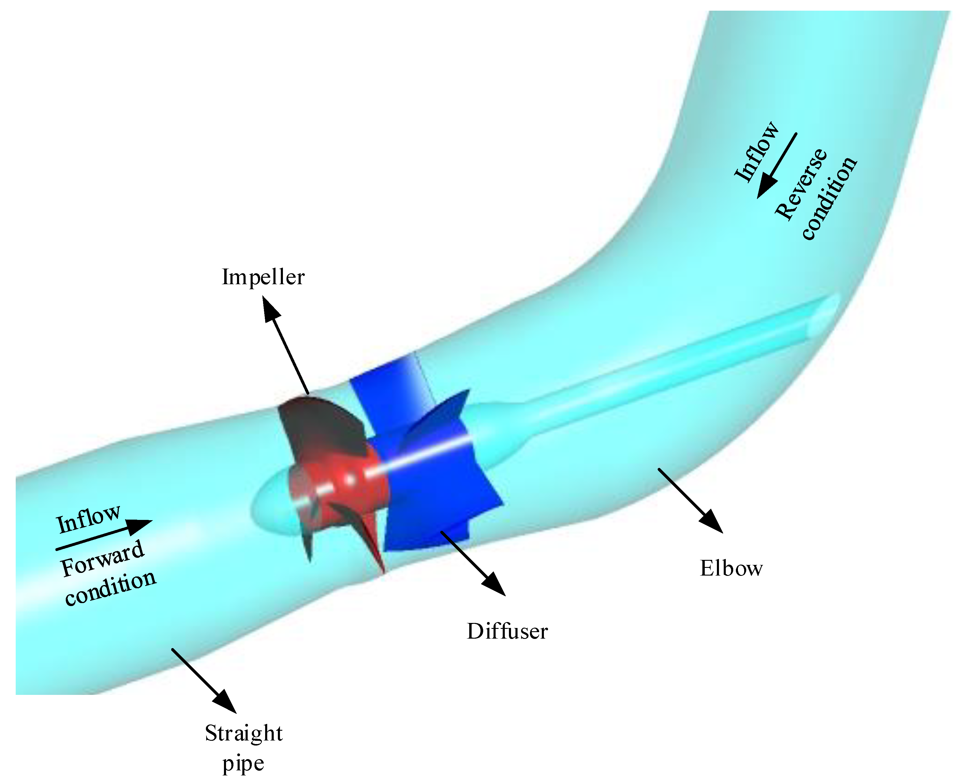
Figure 1.
3D model of the original design.
Figure 1.
3D model of the original design.
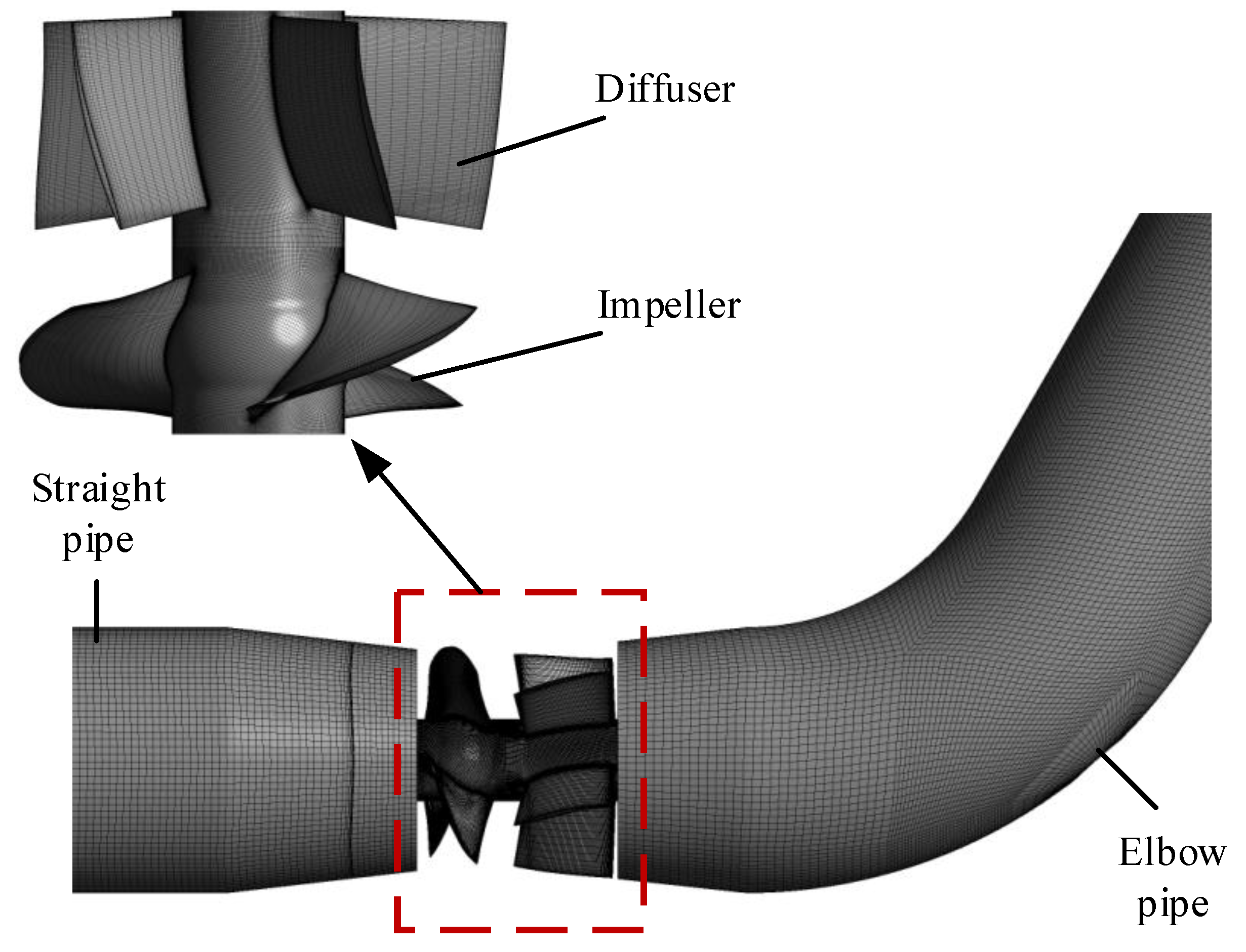
Figure 2.
Mesh of the original design.
Figure 2.
Mesh of the original design.
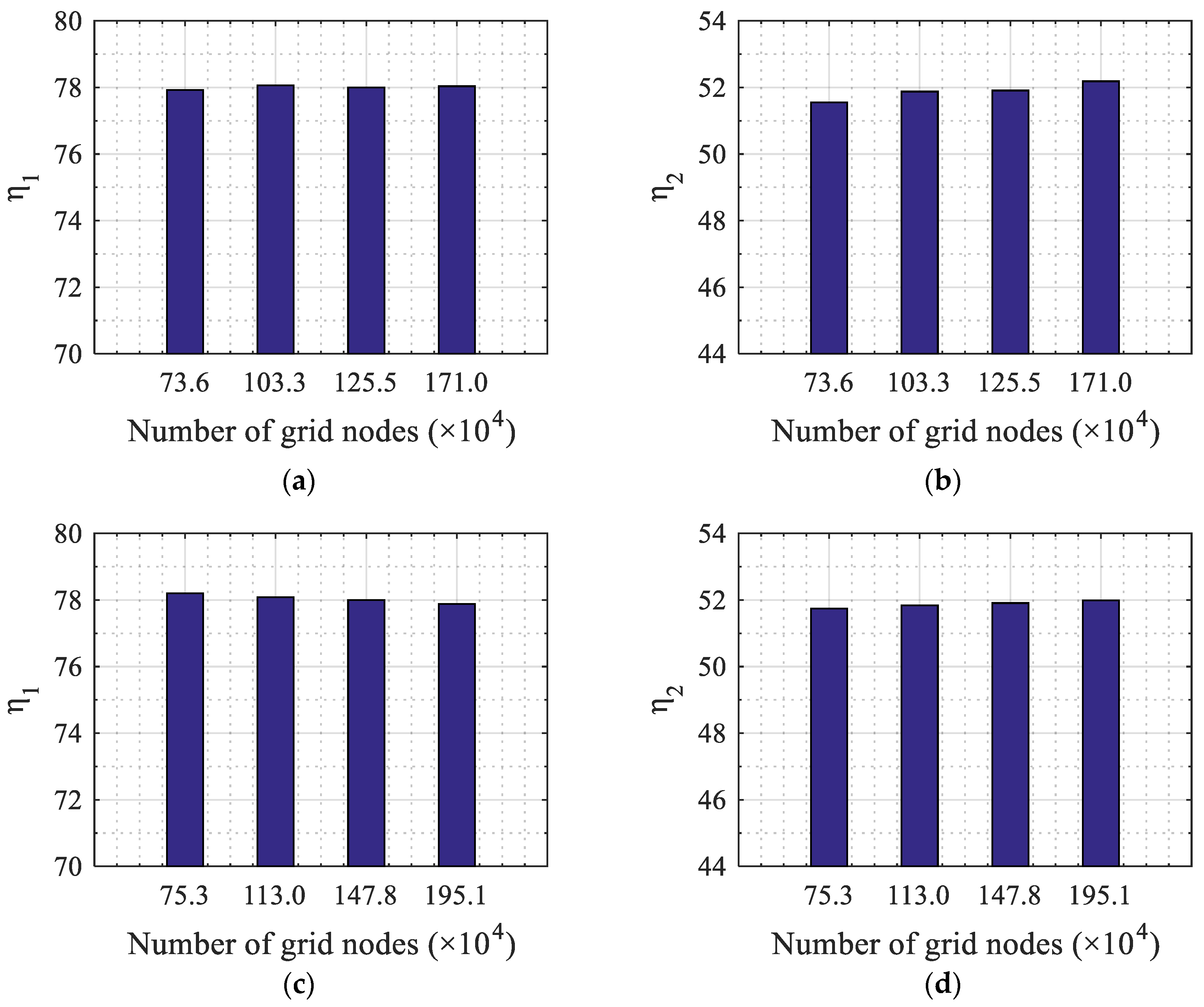
Figure 3.
Grid independence of the original design for the (a) impeller under a forward design flowrate, (b) impeller under a reverse design flow rate, (c) diffuser under a forward design flowrate and (d) diffuser under a reverse design flow rate.
Figure 3.
Grid independence of the original design for the (a) impeller under a forward design flowrate, (b) impeller under a reverse design flow rate, (c) diffuser under a forward design flowrate and (d) diffuser under a reverse design flow rate.
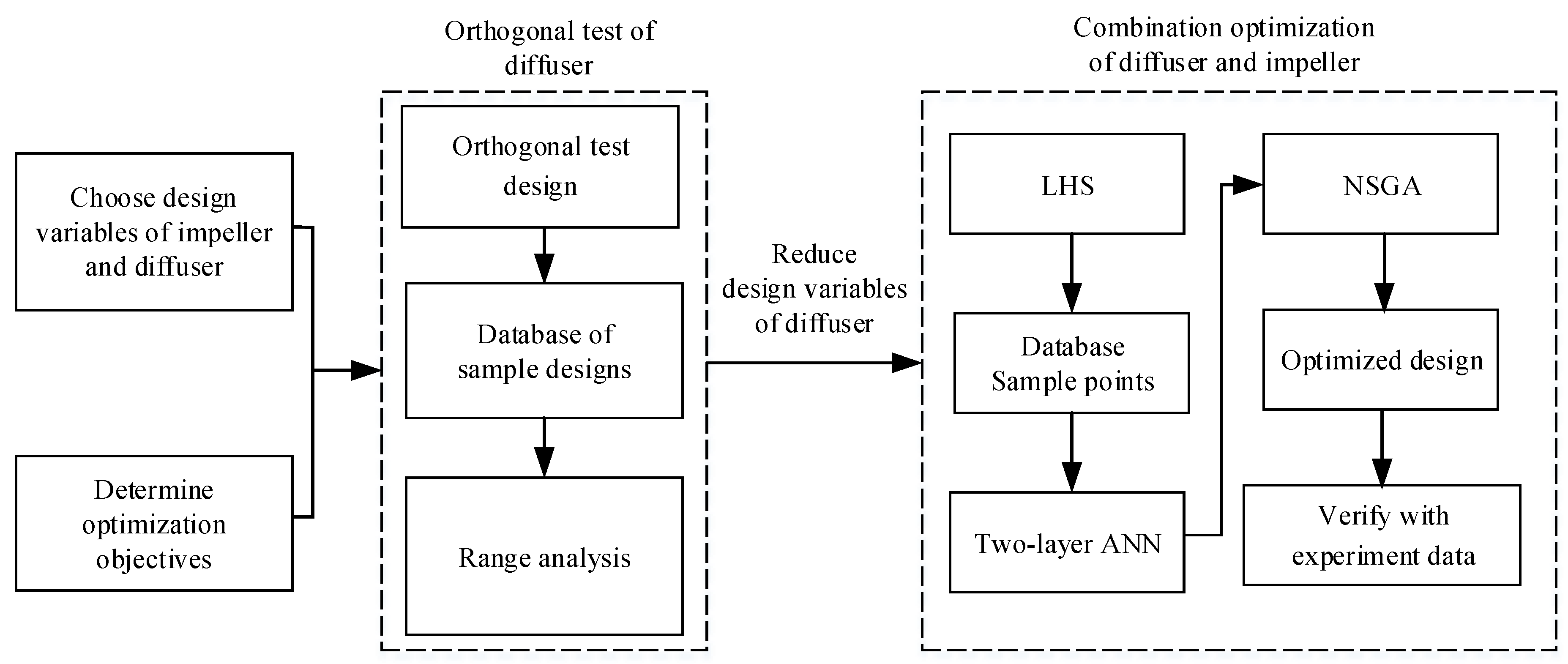
Figure 4.
The optimization procedure of the reversible axial-flow pump.
Figure 4.
The optimization procedure of the reversible axial-flow pump.
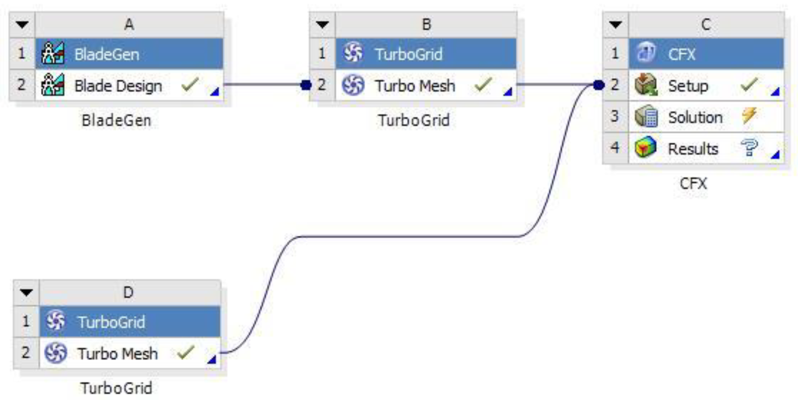
Figure 5.
Optimization flow chart in the ANSYS Workbench.
Figure 5.
Optimization flow chart in the ANSYS Workbench.
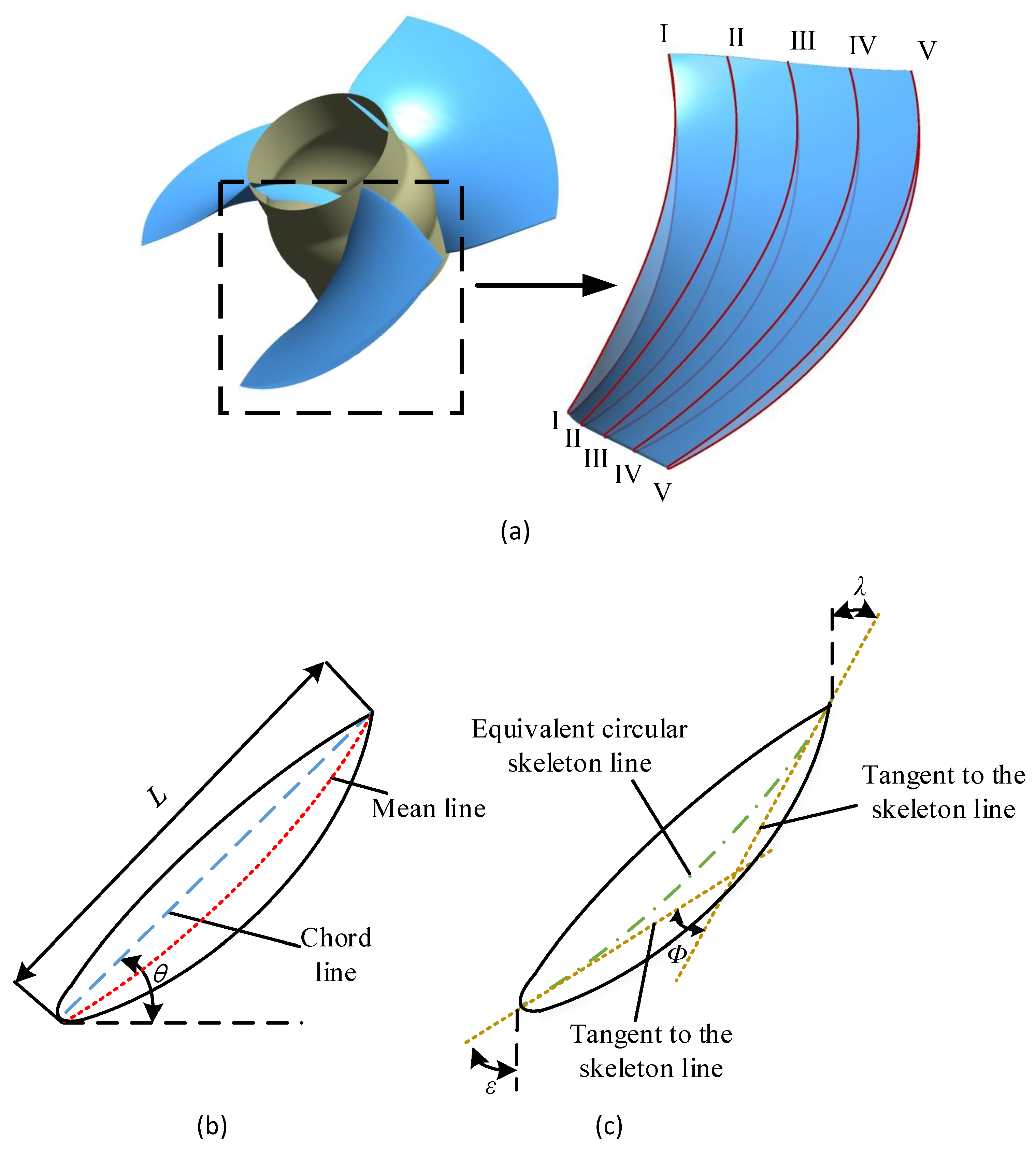
Figure 6.
The definition of the main geometry variables of the impeller: (a) definition of the airfoil section, (b) main geometry variables of the airfoil and (c) the rest of the geometry variables.
Figure 6.
The definition of the main geometry variables of the impeller: (a) definition of the airfoil section, (b) main geometry variables of the airfoil and (c) the rest of the geometry variables.
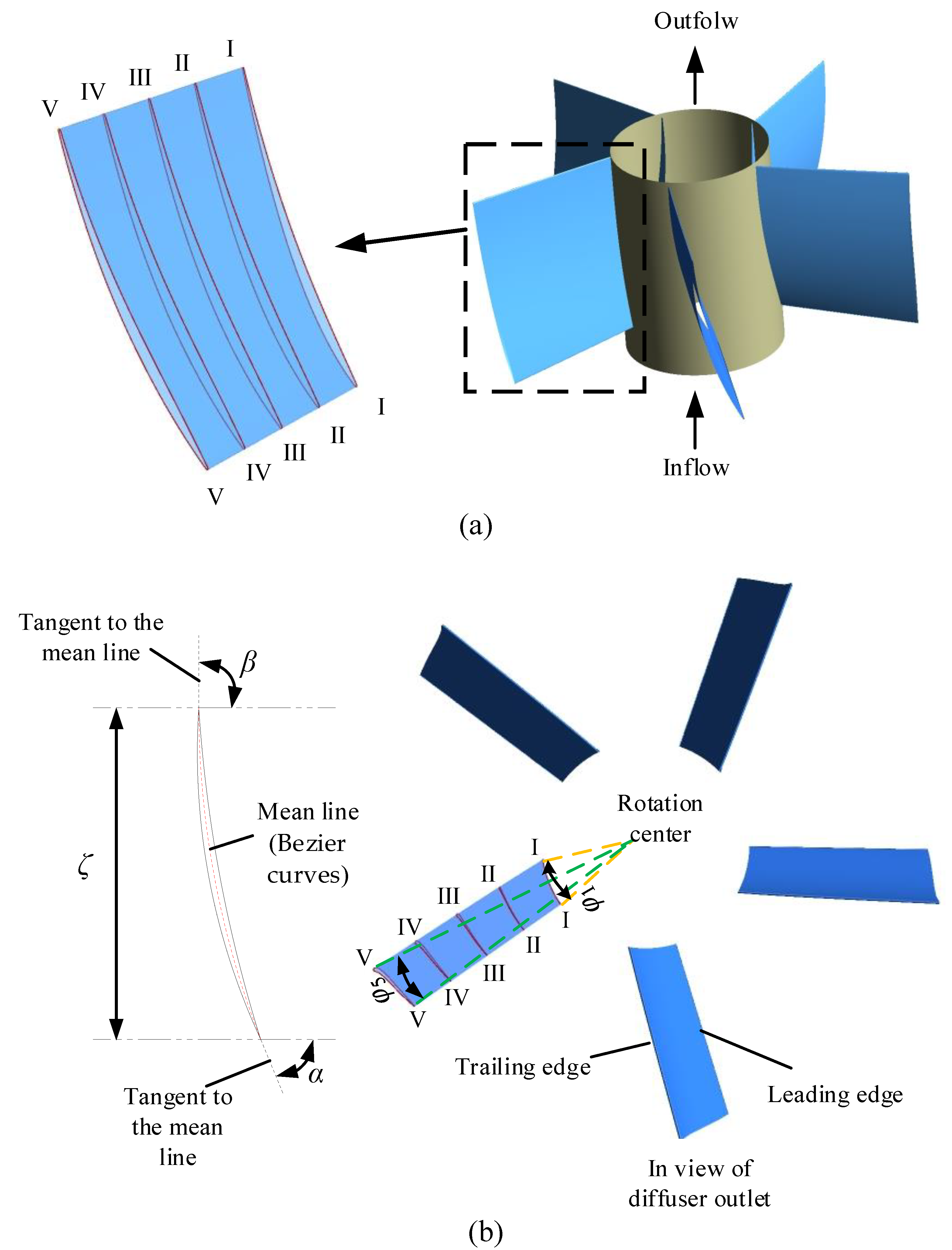
Figure 7.
The definition of the main geometry variables of the diffuser: (a) definition of the airfoil section and (b) main geometry variables of the airfoil.
Figure 7.
The definition of the main geometry variables of the diffuser: (a) definition of the airfoil section and (b) main geometry variables of the airfoil.
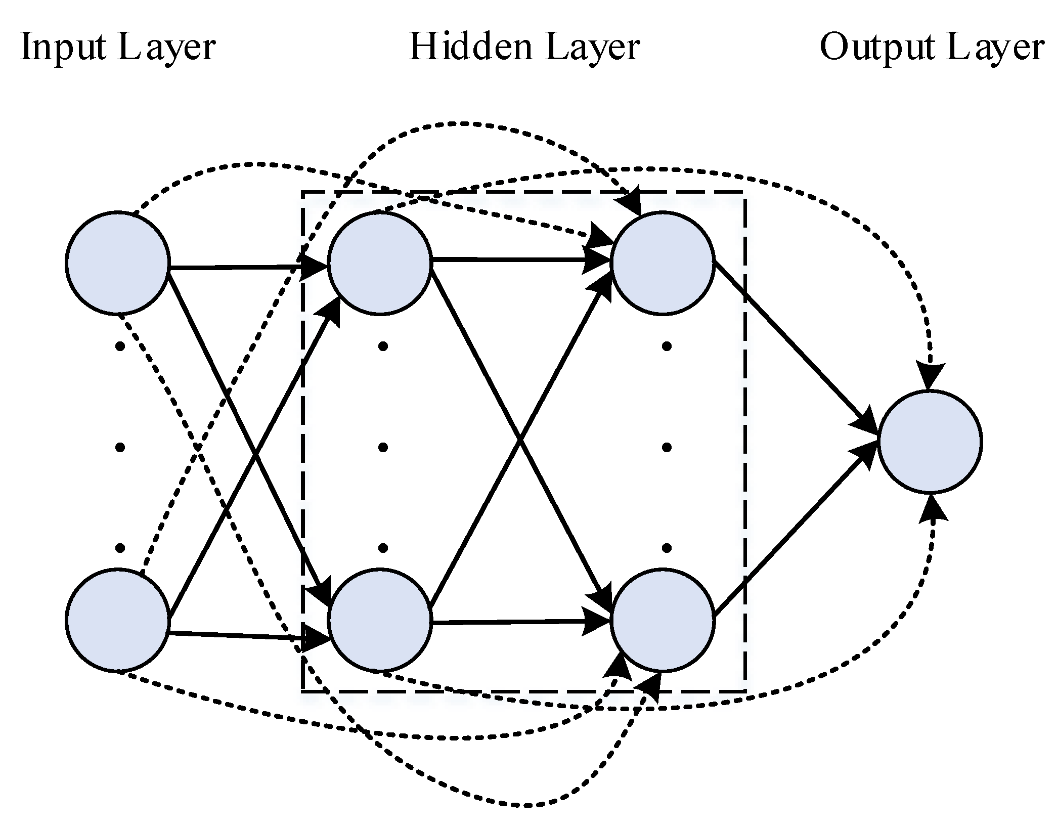
Figure 8.
The structure of the cascade-forward multilayer neural network.
Figure 8.
The structure of the cascade-forward multilayer neural network.
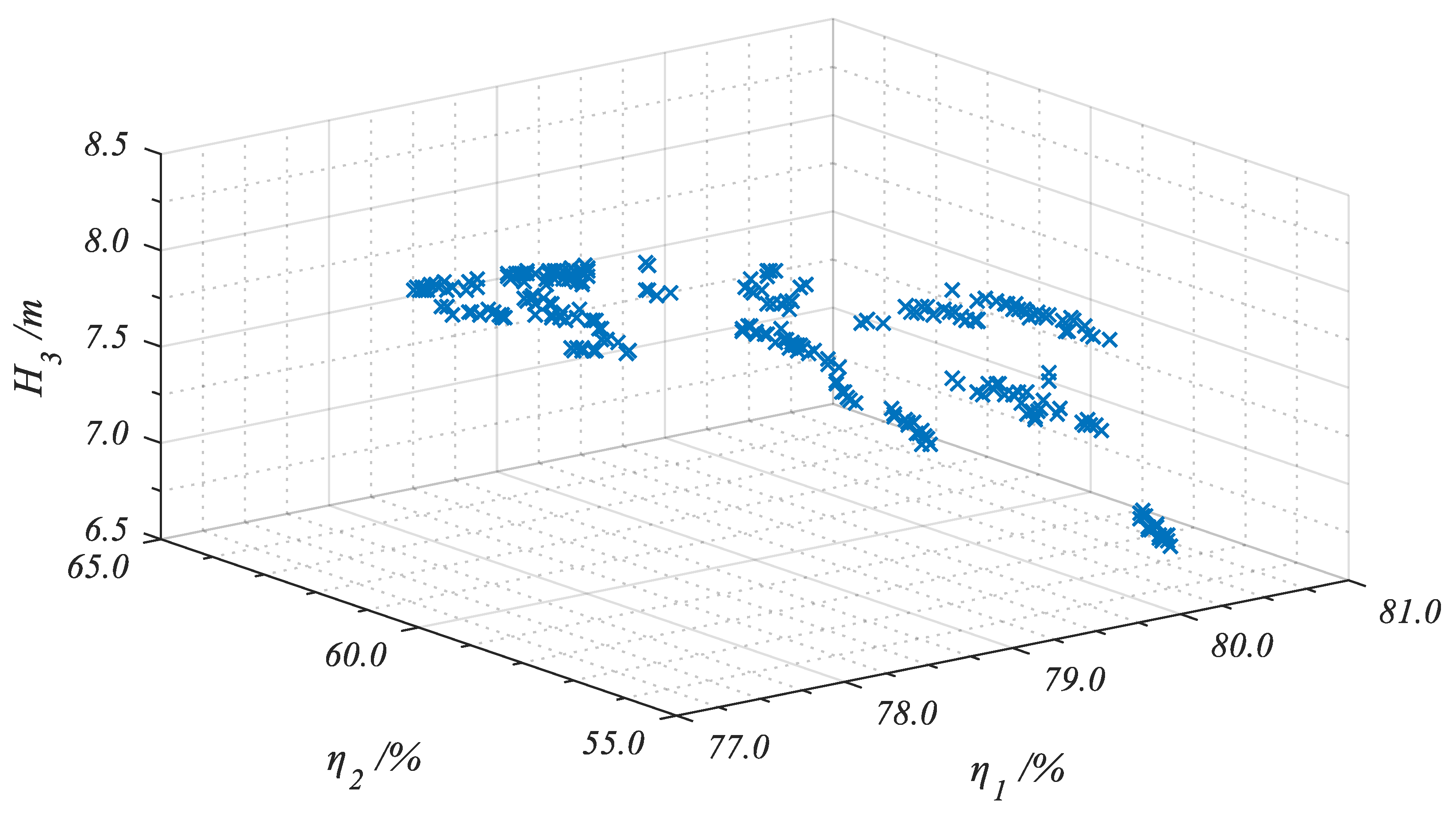
Figure 9.
Pareto-optimal solutions in 3D function-space.
Figure 9.
Pareto-optimal solutions in 3D function-space.
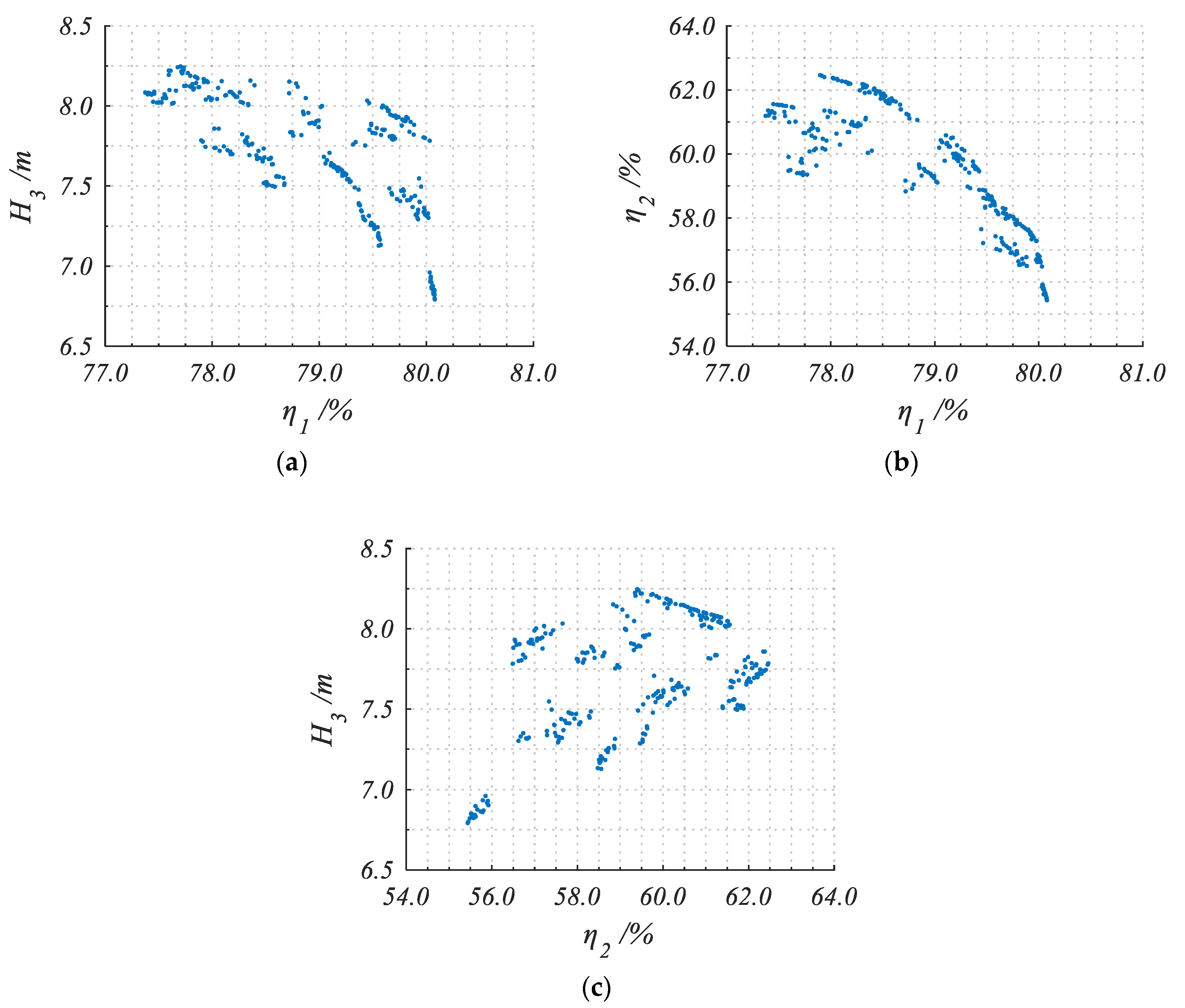
Figure 10.
Pareto-optimal solutions in 2D function-space: (a) , (b) (c) .
Figure 10.
Pareto-optimal solutions in 2D function-space: (a) , (b) (c) .
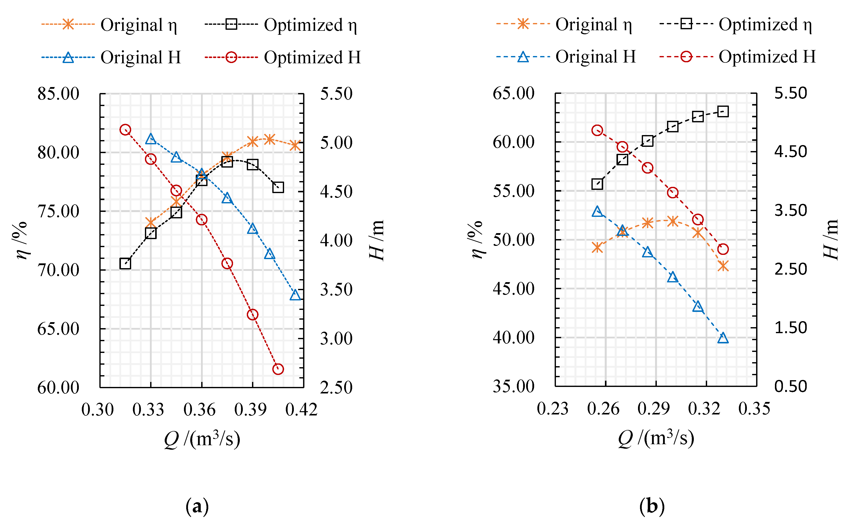
Figure 11.
Comparison of pump performance between the original and optimized design: (a) under the forward condition and (b) under the reverse condition.
Figure 11.
Comparison of pump performance between the original and optimized design: (a) under the forward condition and (b) under the reverse condition.
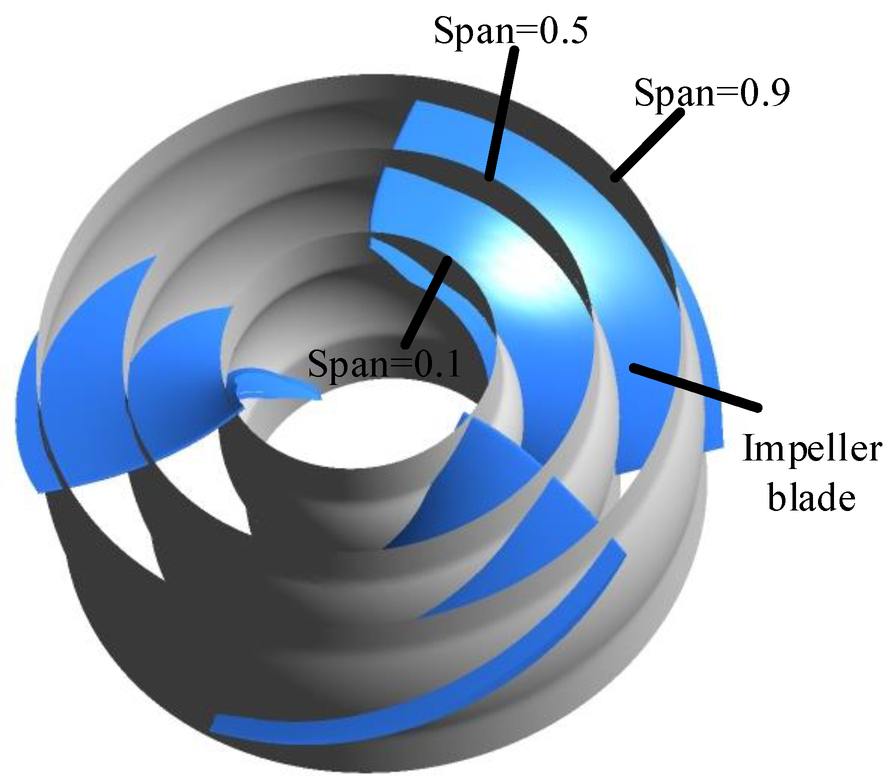
Figure 12.
The turbo surface with different spans.
Figure 12.
The turbo surface with different spans.
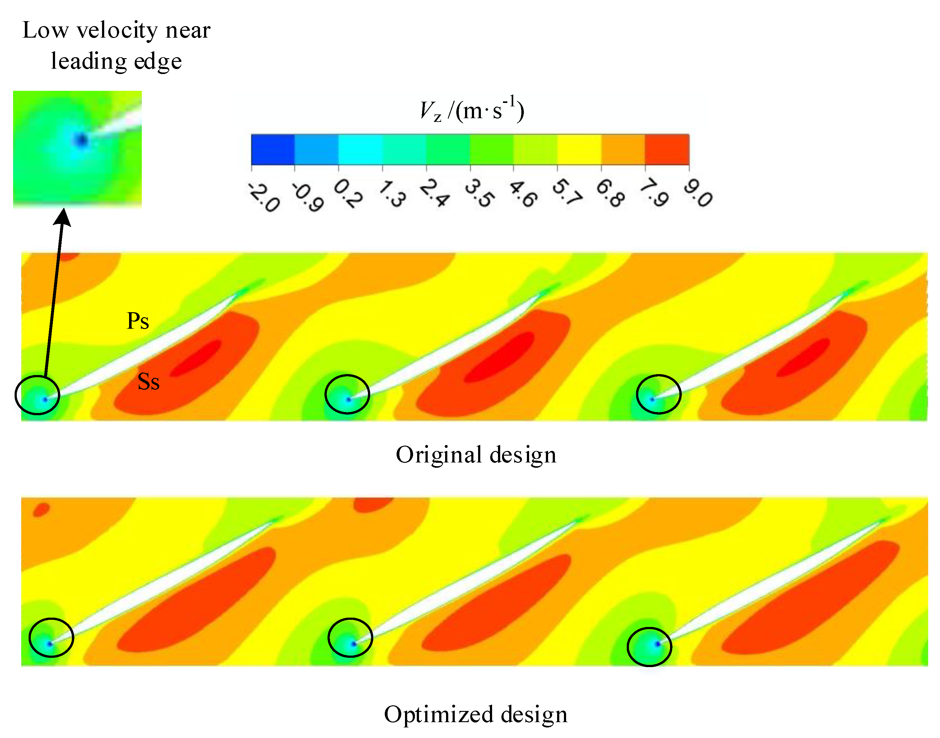
Figure 13.
Comparison of the velocity axial distribution in the impeller between the original design and optimized design under the forward design flow rate (span = 0.5).
Figure 13.
Comparison of the velocity axial distribution in the impeller between the original design and optimized design under the forward design flow rate (span = 0.5).
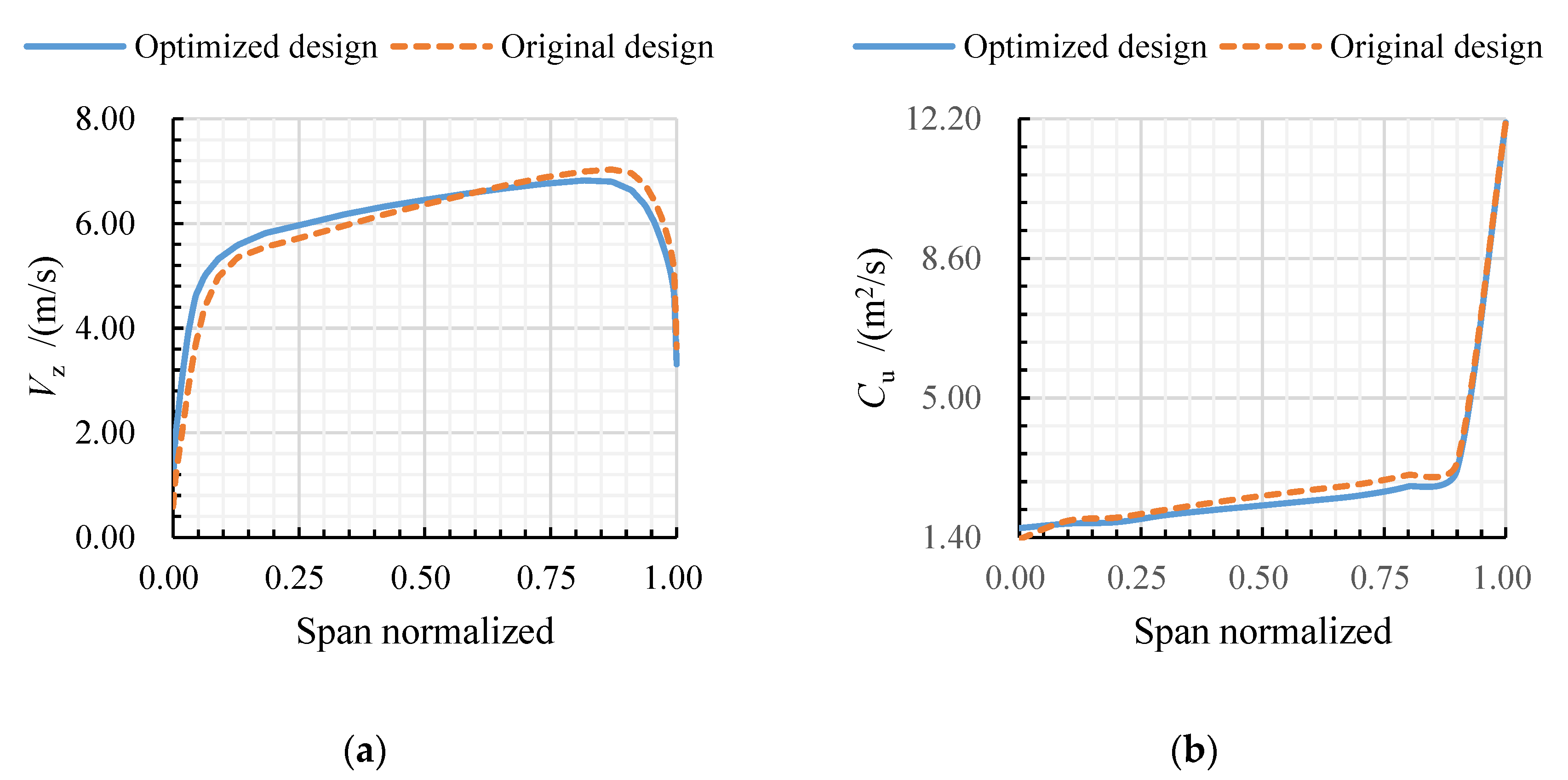
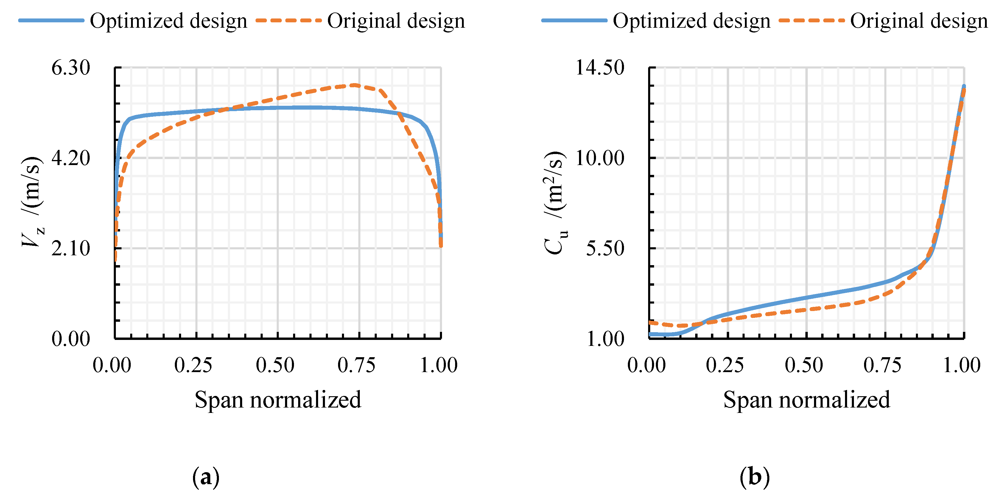
Figure 14.
Comparison in the impeller outlet between the original and optimized design for the (a) velocity axial distribution and (b) circulation distribution (under the forward design flow rate).
Figure 14.
Comparison in the impeller outlet between the original and optimized design for the (a) velocity axial distribution and (b) circulation distribution (under the forward design flow rate).
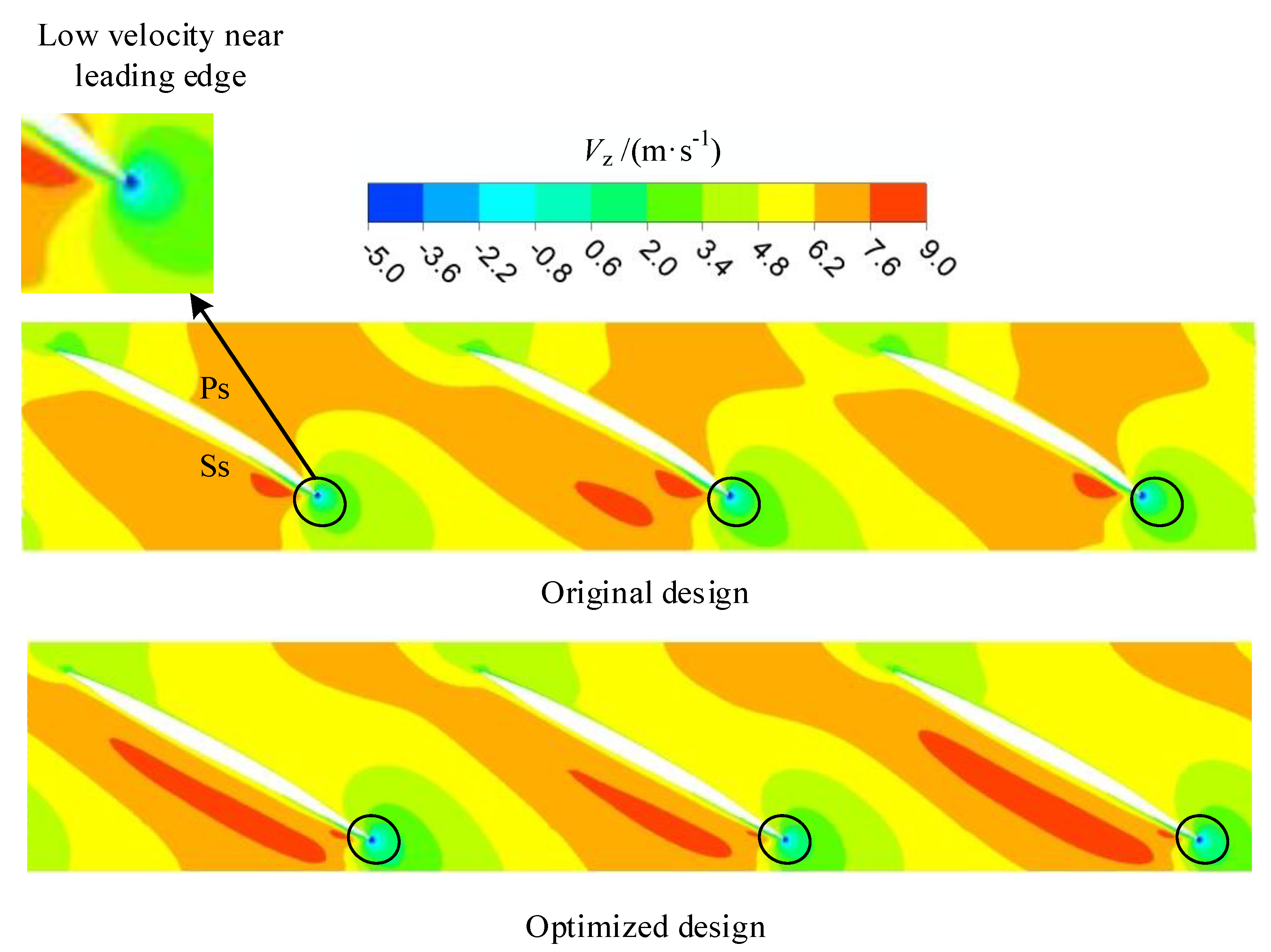
Figure 15.
Comparison of the velocity axial distribution in the diffuser between the original and optimized design under the forward design flow rate (span = 0.5).
Figure 15.
Comparison of the velocity axial distribution in the diffuser between the original and optimized design under the forward design flow rate (span = 0.5).
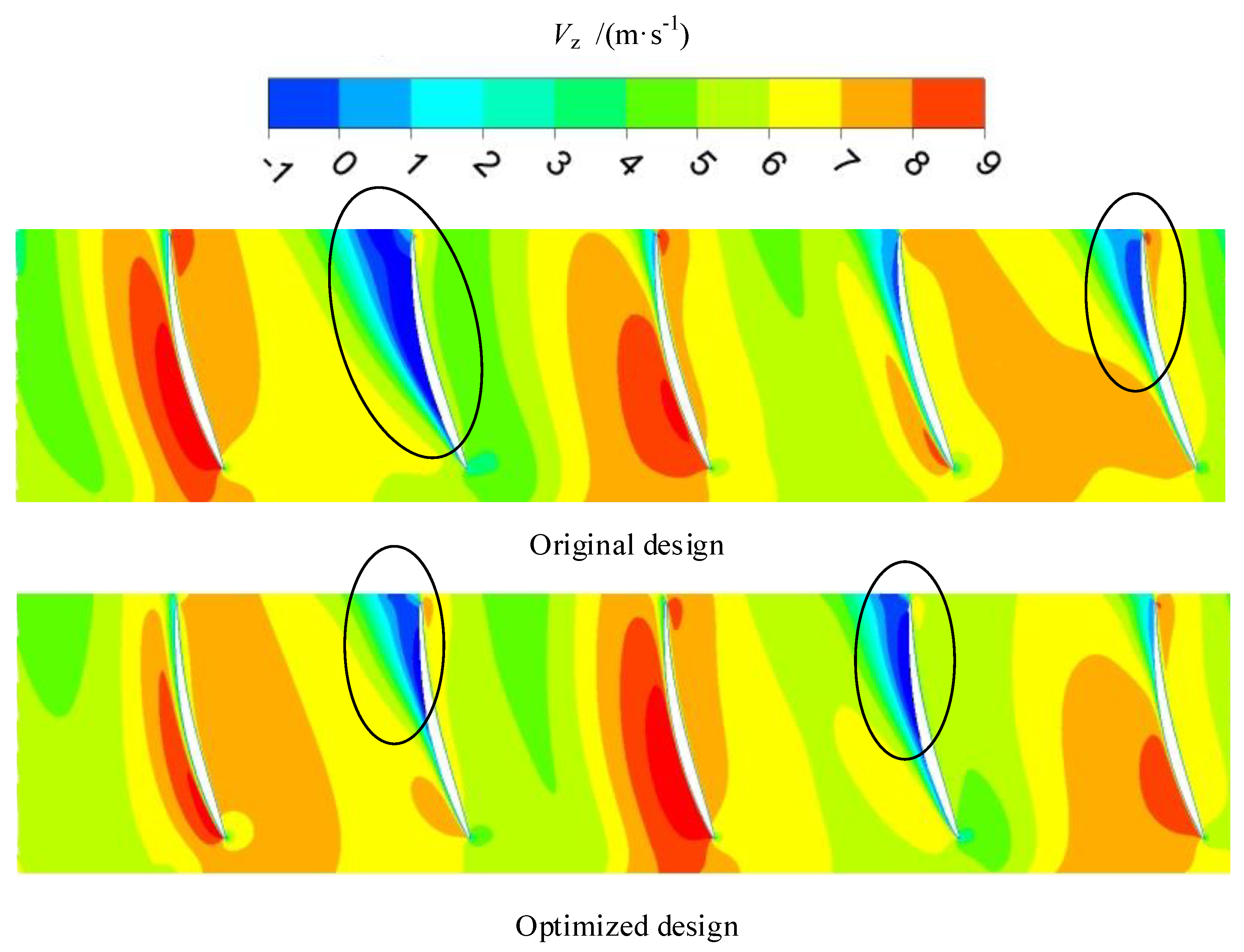
Figure 16.
Comparison of the velocity distribution in the impeller between the original design and optimized design under the reverse design flow rate (span = 0.5).
Figure 16.
Comparison of the velocity distribution in the impeller between the original design and optimized design under the reverse design flow rate (span = 0.5).
Figure 17.
Comparison in the impeller outlet between the original and optimized design for the (a) axial velocity distribution and (b) circumferential velocity distribution (under the reverse design flow rate).
Figure 17.
Comparison in the impeller outlet between the original and optimized design for the (a) axial velocity distribution and (b) circumferential velocity distribution (under the reverse design flow rate).
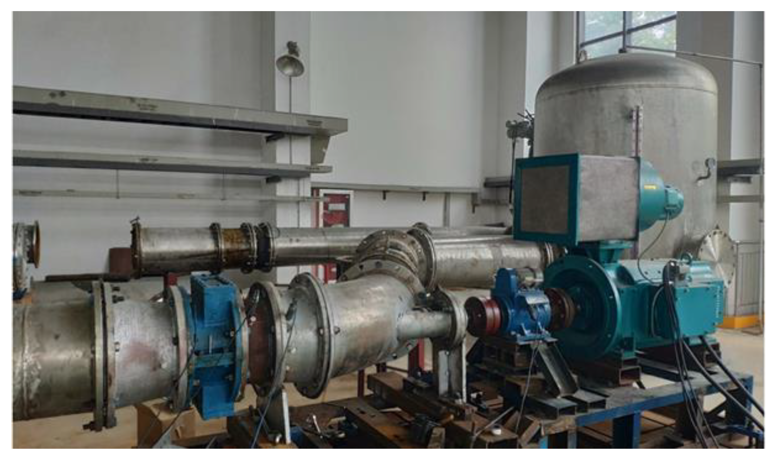
Figure 18.
The experiment bench of the axial-flow pump.
Figure 18.
The experiment bench of the axial-flow pump.
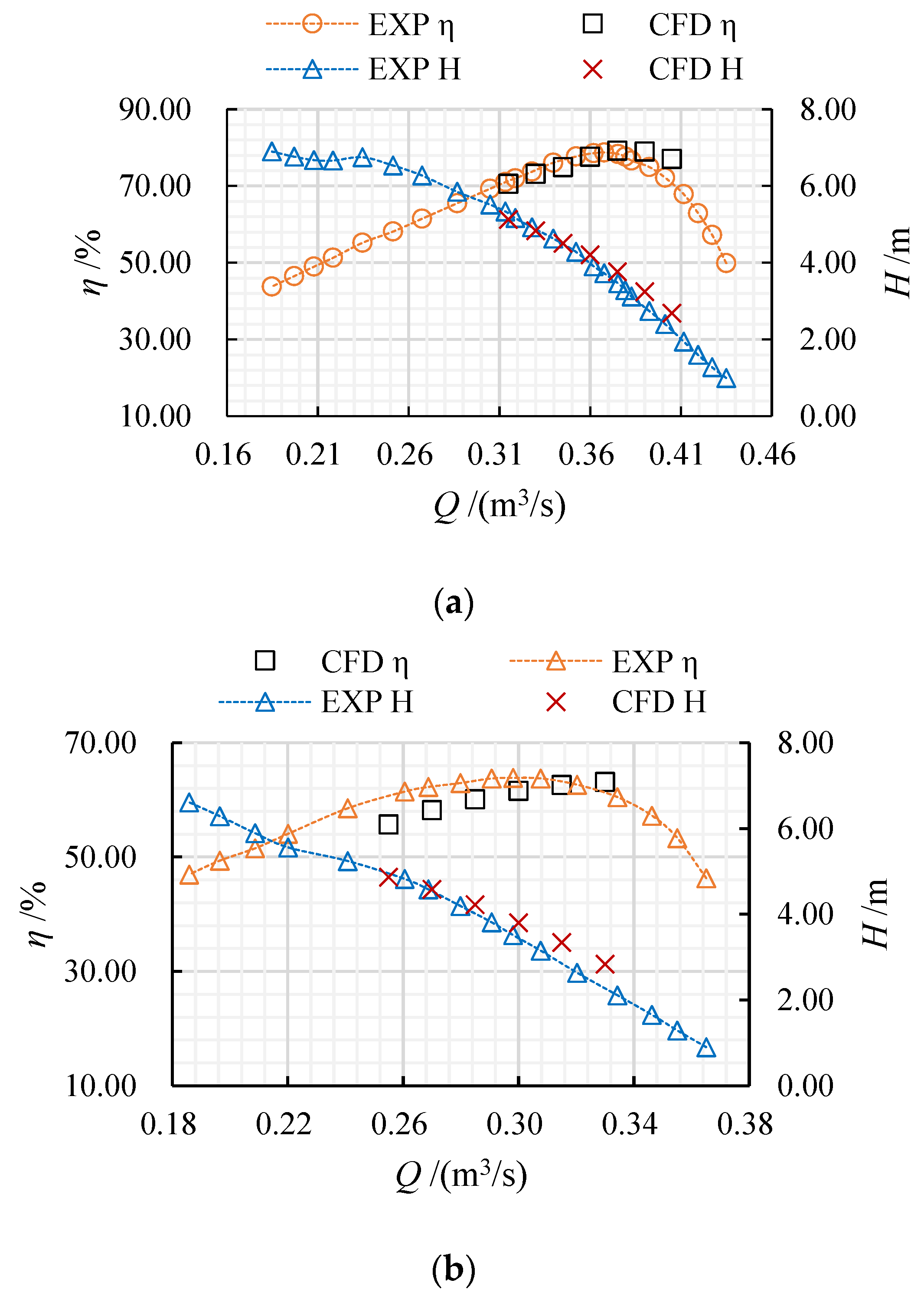
Figure 19.
The comparison of pump performance between the simulated data and experiment data under the (a) forward operation and (b) reverse operation.
Figure 19.
The comparison of pump performance between the simulated data and experiment data under the (a) forward operation and (b) reverse operation.
Table 1.
Main parameters of the original design.
Table 1.
Main parameters of the original design.
| Design Parameters |
| Rated flow rate (m3/s) | 0.4 | Rotational speed (r/min) | 1450 |
| Head on rated flow rate (m) | 3.87 | Specific speed | 1213.1 |
| Geometry Parameters |
| Impeller blade number | 3 | Diffuser blade number | 5 |
| Impeller diameter (mm) | 300 | Outlet diameter of diffuser (mm) | 312.8 |
| Optimization Parameters |
| Forward design flow rate (m3/s) | 0.36 | Efficiency on forward design flow rate (%) | 78.0 |
| Reverse design flow rate (m3/s) | 0.3 | Efficiency on reverse design flow rate (%) | 51.91 |
Table 2.
Level of the orthogonal factor.
Table 2.
Level of the orthogonal factor.
| Level | Factor |
|---|
A
| B
| C
| D
|
|---|
| Level 1 | 70 | 85 | 26 | 4.5 |
| Level 2 | 65 | 80 | 30 | 6.5 |
| Level 3 | 60 | 75 | 34 | 8.5 |
| Level 4 | 55 | 70 | 38 | 10.5 |
| Level 5 | 50 | 65 | 42 | 12.5 |
Table 3.
Orthogonal test scheme.
Table 3.
Orthogonal test scheme.
| Test Number | Factor | Corresponding Parameter | Optimization Objective |
|---|
| A | B | C | D | | | | | | | |
|---|
| 1 | A1 | B1 | C1 | D1 | 70 | 85 | 26 | 4.5 | 73.62 | 54.04 | 7.30 |
| 2 | A1 | B2 | C2 | D2 | 70 | 80 | 30 | 6.5 | 75.43 | 53.30 | 7.21 |
| 3 | A1 | B3 | C3 | D3 | 70 | 75 | 34 | 8.5 | 76.86 | 52.30 | 7.12 |
| 4 | A1 | B4 | C4 | D4 | 70 | 70 | 38 | 10.5 | 77.85 | 51.12 | 6.99 |
| 5 | A1 | B5 | C5 | D5 | 70 | 65 | 42 | 12.5 | 78.90 | 49.69 | 6.88 |
| 6 | A2 | B1 | C2 | D3 | 65 | 85 | 30 | 8.5 | 75.98 | 52.52 | 7.17 |
| 7 | A2 | B2 | C3 | D4 | 65 | 80 | 34 | 10.5 | 77.37 | 51.52 | 7.06 |
| 8 | A2 | B3 | C4 | D5 | 65 | 75 | 38 | 12.5 | 78.79 | 50.31 | 6.98 |
| 9 | A2 | B4 | C5 | D1 | 65 | 70 | 42 | 4.5 | 77.75 | 51.23 | 6.99 |
| 10 | A2 | B5 | C1 | D2 | 65 | 65 | 26 | 6.5 | 77.32 | 51.96 | 7.03 |
| 11 | A3 | B1 | C3 | D5 | 60 | 85 | 34 | 12.5 | 77.74 | 50.73 | 7.00 |
| 12 | A3 | B2 | C4 | D1 | 60 | 80 | 38 | 4.5 | 76.43 | 51.75 | 7.03 |
| 13 | A3 | B3 | C5 | D2 | 60 | 75 | 42 | 6.5 | 78.22 | 50.53 | 6.94 |
| 14 | A3 | B4 | C1 | D3 | 60 | 70 | 26 | 8.5 | 77.92 | 51.34 | 7.01 |
| 15 | A3 | B5 | C2 | D4 | 60 | 65 | 30 | 10.5 | 79.38 | 49.85 | 6.92 |
| 16 | A4 | B1 | C4 | D2 | 55 | 85 | 38 | 6.5 | 76.96 | 50.95 | 6.98 |
| 17 | A4 | B2 | C5 | D3 | 55 | 80 | 42 | 8.5 | 78.45 | 49.66 | 6.87 |
| 18 | A4 | B3 | C1 | D4 | 55 | 75 | 26 | 10.5 | 78.54 | 50.45 | 6.96 |
| 19 | A4 | B4 | C2 | D5 | 55 | 70 | 30 | 12.5 | 79.82 | 48.90 | 6.85 |
| 20 | A4 | B5 | C3 | D1 | 55 | 65 | 34 | 4.5 | 77.64 | 49.81 | 6.79 |
| 21 | A5 | B1 | C5 | D4 | 50 | 85 | 42 | 10.5 | 78.77 | 48.56 | 6.80 |
| 22 | A5 | B2 | C1 | D5 | 50 | 80 | 26 | 12.5 | 79.06 | 49.67 | 6.91 |
| 23 | A5 | B3 | C2 | D1 | 50 | 75 | 30 | 4.5 | 77.19 | 50.54 | 6.87 |
| 24 | A5 | B4 | C3 | D2 | 50 | 70 | 34 | 6.5 | 78.47 | 49.07 | 6.76 |
| 25 | A5 | B5 | C4 | D3 | 50 | 65 | 38 | 8.5 | 80.34 | 47.07 | 6.69 |
Table 4.
Range analysis of
Table 4.
Range analysis of
| Test Indices | D | A | B | C |
|---|
| K1 | 382.63 | 382.66 | 383.08 | 386.45 |
| K2 | 386.41 | 387.21 | 386.73 | 387.81 |
| K3 | 389.54 | 389.70 | 389.60 | 388.08 |
| K4 | 391.90 | 391.41 | 391.81 | 390.37 |
| K5 | 394.32 | 393.83 | 393.59 | 392.10 |
| 76.53 | 76.53 | 76.62 | 77.29 |
| 77.28 | 77.44 | 77.35 | 77.56 |
| 77.91 | 77.94 | 77.92 | 77.62 |
| 78.38 | 78.28 | 78.36 | 78.07 |
| 78.86 | 78.77 | 78.72 | 78.42 |
| R | 2.34 | 2.23 | 2.10 | 1.13 |
Table 5.
Range analysis of
Table 5.
Range analysis of
| Test Indices | A | B | D | C |
|---|
| K1 | 260.45 | 256.80 | 257.38 | 257.45 |
| K2 | 257.55 | 255.90 | 255.81 | 255.10 |
| K3 | 254.20 | 254.14 | 252.88 | 253.44 |
| K4 | 249.76 | 251.65 | 251.50 | 251.21 |
| K5 | 244.91 | 248.38 | 249.30 | 249.68 |
| 52.09 | 51.36 | 51.48 | 51.49 |
| 51.51 | 51.18 | 51.16 | 51.02 |
| 50.84 | 50.83 | 50.58 | 50.69 |
| 49.95 | 50.33 | 50.30 | 50.24 |
| 48.98 | 49.68 | 49.86 | 49.94 |
| R | 3.11 | 1.68 | 1.62 | 1.55 |
Table 6.
Range analysis of
Table 6.
Range analysis of
| Test Indices | A | B | C | D |
|---|
| K1 | 35.51 | 35.25 | 35.22 | 34.98 |
| K2 | 35.24 | 35.09 | 35.03 | 34.93 |
| K3 | 34.90 | 34.87 | 34.72 | 34.85 |
| K4 | 34.45 | 34.60 | 34.67 | 34.73 |
| K5 | 34.03 | 34.31 | 34.49 | 34.62 |
| 7.10 | 7.05 | 7.04 | 7.00 |
| 7.05 | 7.02 | 7.01 | 6.99 |
| 6.98 | 6.97 | 6.94 | 6.97 |
| 6.89 | 6.92 | 6.93 | 6.95 |
| 6.81 | 6.86 | 6.90 | 6.92 |
| R | 0.30 | 0.19 | 0.14 | 0.07 |
Table 7.
The accuracy of optimization objective predicted by different approximation models.
Table 7.
The accuracy of optimization objective predicted by different approximation models.
| Approximation Model | | | | |
|---|
| Two-layer ANN Model | 0.982 | 0.990 | 0.993 | 0.996 |
| RSM | 0.913 | 0.962 | 0.970 | 0.994 |
| Kriging Model | 0.792 | 0.953 | 0.938 | 0.948 |
| RBF Model | 0.905 | 0.983 | 0.972 | 0.993 |
Table 8.
Main technical parameters of measurement equipment.
Table 8.
Main technical parameters of measurement equipment.
| Measurement Items | Equipment Name | Instrument Model | Measurement Range | Measurement Accuracy |
|---|
| Flow rate | Intelligent electromagnetic flowmeter | OPTIFLUX2000F | 0–1800 m3/h | <±0.2% |
| Head | Intelligent differential pressure transmitter | EJA | 0–10 m | <±0.1% |
| Torque | Intelligent torque speed sensor | JCL1 | 0–200 N·m | <±0.1% |
| Rotation speed |
Table 9.
The main design parameters of the optimized reversible axial-flow pump.
Table 9.
The main design parameters of the optimized reversible axial-flow pump.
| Design Parameters | Value |
|---|
| Forward rated flowrate (m3/s) | 0.368 |
| Efficiency under forward rated condition (%) | 78.73 |
| Head under forward rated condition (m) | 3.72 |
| Reverse rated flowrate (m3/s) | 0.298 |
| Efficiency under reverse rated condition (%) | 63.85 |
| Head under reverse rated condition (m) | 3.51 |
| Rotation speed (rev/min) | 1450 |

 ,
, 


